A Performance Evaluation of Modified Weighted Pathloss Scenario Based on the Cluster Based-PLE for an Indoor Positioning of Wireless Sensor Network

(1)

A Performance Evaluation of Modified Weighted Pathloss Scenario

Based on the Cluster Based-PLE for an Indoor Positioning of

Wireless Sensor Network

Cindha Riri Pratiwi

1,*

, Prima Kristalina

2

, Amang Sudarsono

2

1_{Graduate School of Electrical Engineering, Politeknik Elektronika Negeri Surabaya, Institute of Surabaya, Indonesia} 2

Department of Electrical Engineering, Politeknik Elektronika Negeri Surabaya, Institute of Surabaya, Indonesia

Received 31 March 2017; received in revised form 04 September 2017; accepted 09 October 2017

Abstract

The indoor positioning system is one of the popular topics in the current study; it is mainly due to the inability

of the Global Positioning System (GPS) applied inside a building. LANDMARC (Location Identification based on

Dynamic Active RFID Calibration) and Enhanced LANDMARC Scenario use calibration RSSI values and weighted

process to obtain accuracy of position estimation. Meanwhile, WPL (Weighted Pathloss) method improves the

positioning accuracy of the two previous methods (LANDMARC and Enhanced LANDMARC) by observing the

Path Loss Exponent (PLE) value in an indoor environment, followed by using the value to estimate the object

position. We propose a Modified WPL uses Cluster Based Pathloss Exponent (PLE) method by combining the

functions of the existing calibration in LANDMARC Scenario with the Cluster Based PLE value. The test bed was

conducted in an indoor area on the 3rd floor of the PENS Postgraduate Building. The nodes were connected to each

other using X-Bee Pro S2 module. RSSI (Received Signal Strength Indicator) value was used to estimate the distance

between transmitter and receiver nodes. The result of the MSE estimation position using the proposed method was

3.80 meters, whereas WPL method was 5.78 meters. Overall, the proposed Modified WPL with Cluster Based PLE

method showed that it had the capability to enhance the accuracy of localization; 34% better than the standard WPL

method.

Keywords: indoor positioning system, LANDMARC, WPL, cluster based PLE

1. Introduction

Wireless Sensor Network (WSN) becomes an interesting topic among the research community and industry. There are a

lot of applications that could be built with the WSN such as monitoring, tracking, healthy monitoring robotics applications and

so on [1]. In monitoring and tracking applications, WSN can be used to estimate the distance between an object and its

monitoring system, also, locate the position of object or personnel [2-4]. Spotting the position of a mobile object or person is an

interesting and challenging problem in WSN. In an outdoor environment, the position or location of an object could be

monitored or tracked by Global Position System (GPS), but the problem occurs when the position of the object is located in an

indoor environment. In general, GPS needs a strong signal to connect to a satellite; however, in an indoor environment, the

signal strength will decrease, due to blockage from the roof or other material [5]. Based on distance measurement, there are two

categories of localization techniques, i.e. range-based localization [6] which uses measurement instruments or tools to estimate

the distance between transmitter and receiver nodes, and a range free localization [7]. There are no measurement instruments

to determine the distance of two or more nodes.

(2)

Currently, distance measurements use various types of instruments, such as Ultrasonic distance measurement methods,

Receive Signal Strength Indicator (RSSI) [8-9], Time of Arrival (TOA) [8,10], Time Different of Arrival (TDOA) [8,11] and

Angle of Arrival (AOA) [8,9]. In consideration of the cost aspect, power consumption, and simplification of localized system,

we choose RSSI technique for the proposed indoor localization algorithm. In our scheme, we used a pair of nodes. The first

node serves as the transmitter node: while the other serves as the receiver node. Unfortunately, in a real system, there are many

uncertainties in the magnitude of arriving signal due to the influence of environmental factors. These factors are shadowing,

multi-path transmission, reflection, refraction, antenna gain and many other obstacles of indoor environment. This research

believes that the measured value of RSSI decreases as the distance increases. Nonetheless, thecondition might not be achieved

in an indoor area, since the measurement of RSSI value at the distance of more than 12 meters is fluctuating.

In this condition, the estimated distance based on RSSI becomes inaccurate, inconsistent, and will have higher error rate

[12]. To solve this problem, some researchers proposed a statistical filter methodology such as Extended Kalman Filter (EKF)

[13], Particle Swarm Optimization (PSO), Particle Filter (PF) [14-15], and other methodologies to reduce the error in RSSI

value. However, using these filters, the system model must be described accurately. Moreover, the computational complexity

increases, and it is difficult to implement in the real time WSN application.

Based on the previous reasons, the observation area was divided into sub-areas with different Path Loss Exponents (PLEs)

so as to estimate the distance more accurately. The proposed method reaches the ability to solve the fluctuating result of RSSI

measurement and does not make any complexity in computation. Furthermore, the cluster based PLE also improves the

accuracy of estimated distance from RSSI value [16]. This estimated distance resulted from the proposed model can be used to

derive the estimated position of the object by way of using the lateration methods, such as trilateration or multilateration

method [17-18]. Basically, higher error of distance estimation yields a higher error of position estimation. To solve this

problem, the calibration technique can be developed to increase the accuracy of estimated distance and position. A famous

scenario of calibration technique is LANDMARC [19]. The enhancement of LANDMARC and Weighted Path Loss (WPL)

methods is the modified version of LANDMARC. The difference between LANDMARC and WPL method lies in the

calibration method. WPL method did not use calibration method, but instead focuses on finding PLE in the measurement area

[20-21].

In this research, the main purpose of the usage of Cluster Based PLE is to increase the accuracy of estimated distance. The

modification of WPL is on the usage of calibration method that adopts LANDMARC’s. The calibration of received signal

power can be achieved through two steps: the first step is to set the estimated distance of measured received signal power based

on Cluster Based PLE’s value. The second step is to convert back into received signal power by making the estimated distance

into mathematic computation in the observation area. LANDMARC’s method [19] needs 3 kinds of devices, i.e. tracking tag,

reference tag, and reader tag. On a modified WPL, only 2 kinds of devices are needed: a transmitter node as a reference tag and

a receiver node as a tracking tag. In this observation area, the proposed Modified WPL with Cluster Based PLE method not

only enhances the precision of localization accuracy by 30% over LANDMARC, 29% over Enhanced LANDMARC and 23%

over WPL method, but also reduces the number of devices used in the estimation process of position.

2. Related Work

The LANDMARC scenario [19] uses calibration technique for 3 kinds of devices, i.e.: tracking tag, reference tag and

(3)

The Enhanced LANDMARC proposed by [20] still utilizes the calibration technique of repeating error corrections

obtained from RSSI values which measures between the tracking tag and its k nearest reference tags. This method is a recursive data processing approach and needed a certain amount of time to complete the calculation process.

A Weighted Path Loss localization algorithm has been proposed by [21]. This algorithm was claimed to be better than the

two previous methods. The authors mentioned that too many reference tags might increase the RF interferences. Hence, in this

proposed article, they did not require any reference tag in order to address this problem. They used modify ITU (International

Telecommunication Union) indoor Path Loss (PL) equation to calculate the estimated distance between tracking tag and each

sensor, then the estimated location of tracking tag could be obtained by summation of the weighted factor between each sensor

and the tracking tag. The drawback of this method is, that the utilization of Path Loss Exponent for the environment wasn’t

been observed that carefully.

3. Adopted Model and Scenario of Localization Techniques

In this section, the adopted models and the scenarios of localization techniques as our fundamental proposed system are

briefly describle.

3.1. Indoor path loss model and profiling measurement based indoor localization

RSSI value was received by a receiver from each anchor node. There were two devices in this phase, the first device

named the anchor node had the functionality as a transmitter node; the second device named as the unknown node and served

as a receiver node. The RSSI value was generated by the Xbee Pro (S2) module of the anchor node. The farthest distance

between a pair node has the smallest and unstable RSSI value. The next phase in this methodology is the measurement phase.

This phase was performed to acquire the characteristic of observation area which was labeled as cluster based PLE value. This

value was used as a parameter to find the position of the mobile node based on the distance estimation.

The power received of a signal is modeled through the well-known radio-propagation path loss and shadowing model.

The power received on the distance d of a mobile node j has been transmitted from an anchor node i and it can be expressed as in Eq. (1) [22]:

0

( ) ( ) 10 log10

R t l

d

P d P P d n X

d 

    (1)

where Pt is the power transmit in dB, Pl(d0) is power losses in a reference point with the distance d0, usually 1 meter from the

transmitter point, n is a PLE value and Xσ represents a log normal shadow-fading effect. The value of standard deviation Xσ

depends on the characteristic of the environment from the measurement process. This parameter is measured at an anechoic

chamber. The PLE value is based on the condition of the observation area whose measurement has been done. From Eq. (1) the

value of PLE which notated as n is expressed as Eq. (2):

0

( ( ) )/10log10

10

t l

d

P P d X

d

n



 



(2)

and the estimated distance could be calculated as Eq. (3):

0

( ( ) ( ) )/10

10P dR P dR X n

d    (3)

where d is an estimated distance, PR(d0) is the received signal power with a distance d0, PR(d) is a received signal power with a

distance d, Xσ represents a log normal shadow-fading effect and n is PLE (PathLoss Exponent) value refer to a cluster based PLE.

The fluctuating value of RSSI on each measurement process can be used in modelling the slope of line which has gradient

(4)

y a bx (4)

where b is the coefficient of slope line, and this parameter can be substituted to Eq.(1), so that each value of Eq.(4) is derived as [16, 22]:

( )

R

yP d (5)

0 ( )

t l

a P P d X_ (6)

0 10 log10d

b

d

  (7)

x



n

(8)

EIRP (Effective Isotropic Radiated Power) is the value of transmit power (dB) plus transmitter antenna gain (dB) and

receiver antenna gain (dB). For N linear data of RSSI, using the slope line of Eq. (4), the value of a and b can be calculated as in Eq. (9,10) [22]:

1 1 1

2 2

1 1

( )( )

,

( )

N N N

i i i i

i i i

N N

i i

N x y x y

b

N x x

  

 

 





 



(9)

1 1

N N

i i

y x

a b

N N

 









(10)

N is the number of RSSI level from the measurement. The PLE value uses linear regression, n can be obtained by substituting Eq. (4) and Eq. (5), and it is expressed as in Eq.(11) [16]:

10 b

n



(11)

In the Cluster-Based PLE model, the observation area is divided into three sub-areas to measure the PLE value. Thus, the

Eq. (4) will be added with the i index which is stated as the area number, where i



1, 2,3



as shown in Eq. (12)

( ) ( )

y i  a bx i (12)

Therefore, the value of y(i) depends on the change of value x(i). Meanwhile, b is the variance of PLE.

3.2. LANDMARC scenario

LANDMARC [19] has 3 kinds of nodes: tracking tag, reference tag, and reader tag. The LANDMARC approaches

require signal strength information from each tag in a reachable range to readers. LANDMARC scenario has m as RF readers along with k tags as reference tags and u tracking tags as the object being tracked. The reader tags are configured with a continuous mode (continuously reporting the tags that stay in a specified range or cluster) and a detection-range of 1-8

(meaning the reader will scan from range 1-8 and keep repeating the cycle with 30 seconds per range ratio). The LANDMARC

scenario defines the Signal Strength Vector of a tracking/moving tag as expressed in Eq. (13):

1 2

{ , ,... }_i

S S S S (13)

where Si denotes the signal strength of the tracking tag perceived on reader i, where i{1, }k . For the reference tags, the

(5)

1 2 { , ,... }_j





 



(14)

Next, the LANDMARC scenario introduces the Euclidean distance in signal strengths. For each individual tracking tag j, where j{1, }u the formula calculates Euclidean distance in signal strengths as shown in Eq. (15)

2

1 1

( )

u k

l j i

j i

E  S

 





 (15)

where l{1, }m is the Euclidean distance of signal strength (RSSI) between tracking tags and its corresponding reference tag.

E denotes the location correlation between the reference tags and the tracking tags. For example, the nearer reference tag to the tracking tag is supposed to have smaller E value. If there are m reference tags, a tracking tag has its E vector as



1, 2,... m



E E E E . The LANDMARC scenario is to find the nearest tracking tags to neighbors by comparing the different E

values. These Euclidean values are only used to reflect the relation of tags, and then this scenario uses the reported value of

power level to take the place of the signal strength value in the equation.

In this scenario, we used k the nearest reference tags coordination to locate one unknown tag, the LANDMARC scenario used k as the nearest-neighbor algorithm. The unknown tracking tag estimation position (x,y) can be obtained using Eq. (16):

1

( , ) ( , )

k

i i i i

x y w x y





(16)

with w_i is the weighted factor of the i-th reference tag neighbor and (xi,yi) is the location of the i-th reference tag. The choice

of these weighted factors is another design parameter. Giving all k the nearest neighbors with the same weight (e.g. w_i 1/k), it would make a lot of errors. Thus, this scenario determines w_i, depending on the E value of each reference tag, where w_i is a function of the E value of k-nearest neighbor. The formula to obtain w_i in LANMARC scenario is shown in Eq. (17):

2

1 1

1

i

i _k

i i

E w

E

 



(17)

LANDMARC’s approaches provided the least error, which means the reference tag with the smallest E value has the large weight. This may be explained by the fact that the signal strength is proportionally inverse to the square of the distance.

3.3. Enhanced LANDMARC scenario

Enhanced LANDARC [20] is based on two points. The first point is to obtain the coordinate of tracking tag A. Enhanced

LANDMARC used R as a set of tag A and k as the nearest reference tag. Suppose k=4, then R={Tag 1, Tag 2, Tag 3, Tag 4, Tag A}. In the same area and at the same time, the noise and uncertain environmental factor are assumed to be the same for

members in set R. The second point, this method obtains its coordinate according to Tag A and the other k-1 reference tags. For example, this method obtains tag 2’s coordinate according to tag 1, tag 3, tag 4 and tag A.

This method notes that if the computed tag A coordinate in the first time is larger than the real coordinate, then the

reference tag’s coordinate computed by tag A will also be larger. Thus, the difference between the computed reference tag’s

coordinate and the real coordinates can be computed; also, it would be the value used to calibrate the tracking tag’s coordinate.

The calibration is repeated until it yields the smallest error between the estimated position and the real position. This is the

(6)

After the enhanced LANDMARC algorithm obtained the k nearest reference tags and the coordinate of tracking tag (x, y),

it placed these k tags and the tracking tag with the computed coordinate (x,y) in a set. Considering one reference tag as the tracking tag, we obtained its coordinate



x' , '_i y_i



where i

 

1,k according to the coordinate of K members in this set. After the last compute of coordinates of the reference tags, the error can be obtained as shown in Eq. (18):

1

( ' )

k

i i i

i

x w x x



 





1

( ' )

k

i i i

i

y w y y



 





(18)

where (xi, yi) is the real coordinates of reference tags and wi can be obtained using Eq. (17). Finally, Eq. (19) can be used to calibrate the coordinate of the tracking tag (x’, y’).

( ' , ' )x_i y_i   (x x y)(  y) (19)

Put the tracking tag with the computed coordinates ( ', ')x y and the k reference tags in a set and repeat step by step in Eq. (18) until Eq. (19) computed the tracking tag’s coordinate so as to calibrate the tracking tag’s coordinate until the value

becomes more stable. The stable value becomes the final coordinate of the tag.

3.4.…Weighted Path Loss scenario

Weighted Path Loss [21] has two kinds of nodes: an anchor node and an unknown node. In this scenario, the unknown

node can pick up the signal strength of all anchor nodes. To estimate the position of an unknown node, WPL methods define

the signal strength between the unknown node and the anchor node. The real position of an anchor node is defined as (Xi,Yi).

Based on the Indoor Path Loss Model, the power of a received signal strength is explained at sub-section (3.1) and it is shown

in Eq. (1) and (2). The distance between the anchor nodes and the unknown nodes can be expressed as a d vector, which is given as d j = (d 1j , d 2j , d 3j .dA j )T. The weighted factor of the i-th anchor node with respect to the j-th unknown node is defined

as Eq. (20):

1

ij

ij _A

ij i

d w

d  



(20)

Thus, the estimation position of the j-th unknown node (Uj,Vj) is shown at Eq. (21).

1

( , ) ( , )

A

j j ij i i

i

U V w X Y





(21)

The WPL approach largely depends on the Path Loss Exponent α. This experiment is conducted to measure the signal strength values of a different distance from an anchor node and an unknown node using XBee Pro S2 sensor network so as to

find the relation between asignal strength and itsactual distance. We measure a signal strength of anchor node and an unknown

node at 1 meter to 47 meters in the corridor of PENS Postgraduate Building 3th floor, Surabaya. At each location, 50 RSSI

samples were collected in 1 day.

4. The Proposed Modified WPL Cluster Based PLE Method

This research proposes a Modified WPL with Cluster Based PLE (M-WPL), which is expected to improve the accuracy of

the estimated position of the existing mentioned scenario, such as LANDMARC, Enhanced LANDMARC and WPL. As

described in LANDMARC scenario, the propose method used PR(Power Receive) value as the parameter which is critical to

(7)

Postgraduate Building, as shown at Fig. 3. The scenario of proposed method did not involve any reference node from

LANDMARC’s and enhanced LANDMARC. Thus, we employed only 2 kinds of devices: anchor nodes and unknown nodes

The PR value of the proposed method was obtained from the received signal when the communication between anchor

node and unknown node was done. The value was notated as PR1 (in LANDMARC scenario, this value is known as S notation

in Eq. (13)). This value was obtained from the profiling measurement, e.g. the signal strength which was measured in the

measurement phase, from one actual distance (between the anchor and the unknown node) to another distance. The PR2 value is

known as  notation in the LANDMARC scenario as shown in Eq. (14). This value was obtained from the linear regression

model of the measurement data, as depicted with the red line in Fig. 1. We added the 3rd additional process which converted

PR1 value to be the estimated distance using Eq. (3) in Section 3, yielded dˆ. This process is proposed in Cluster-based Path

Loss Exponent (Cluster-Based PLE) method of [21]. The purpose of this process is to obtain the highest accuracy of estimating

distance.

Fig. 1 The relation between the actual distance and the power received at the particular point of distance-with profiling and linear regression model data

The PR2 is a linear model, data derived as a linear equation expressed in Eq. (22). The graph in Fig. 1 shows the

relationship between the actual distance and the power received at the point of actual distance. The graph contains profiling

data, which was measured at the 3rd Floor PENS Postgraduate Building (in doted mark), and linear regression data is shown in the red line.

2 ( 39.82) ( 1.1995)ˆ

R

P     d (22)

Using the two kinds of received signal powers, PR1and PR2, we could calculate the Eucledian distance among them using

Eq. (23):

1 2

1

( ) ( ( ) ( ))

m

R R

i

eu i P i P i





 (23)

where m is the number of distance data. Moreover, eu(i) isused to calculate the weighted factor of each distance from the pair of anchor and unknown node, as shown at Eq. (24).

1

1 ( )

( )

1 ( )

e _A

i

eu i w i

eu i  

(8)

Finally, the estimated position of the mobile unknown node can be calculated as in Eq. (25).

1

( ( ), ( )) ( )( ( ), ( ))

A e i

U j V j w ij X i Y i





(25)

21

5. Experimental Setup and Performance Evaluation

5.1. The scenario of node placement

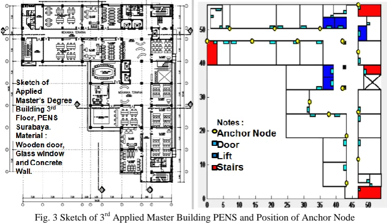
In this work, the 3rd Floor of PENS Postgraduate Building is used as the real indoor environment to set up the

measurement process. 18 anchor nodes and 53 positions of unknown node were deployed within this building, as shown at Fig.

3. The mobile object, in this case, the unknown node was attached to the height of 0.9m and each anchor were attached to the

height of 1.5m. The wireless communication between anchor nodes and unknown node was conducted by Xbee-PRO (S2). The

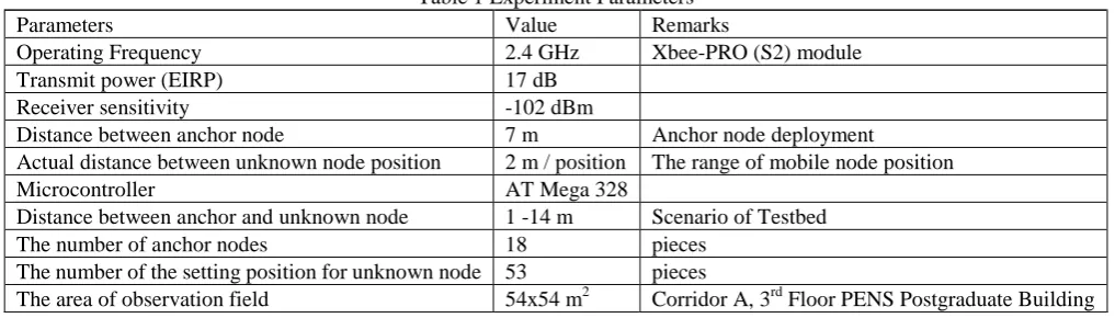
detail of experiment parameters involved in testbed, simulation is listed in Table 1.

Table 1Experiment Parameters

Parameters Value Remarks

Operating Frequency 2.4 GHz Xbee-PRO (S2) module

Transmit power (EIRP) 17 dB

Receiver sensitivity -102 dBm

Distance between anchor node 7 m Anchor node deployment

Actual distance between unknown node position 2 m / position The range of mobile node position

Microcontroller AT Mega 328

Distance between anchor and unknown node 1 -14 m Scenario of Testbed

The number of anchor nodes 18 pieces

The number of the setting position for unknown node 53 pieces

The area of observation field 54x54 m2 Corridor A, 3rd Floor PENS Postgraduate Building

5.2. Measurement phase

The real-time experiment was conducted to measure the signal strength received by unknown node at a certain position.

This signal strength was transmitted by the nearest anchor nodes in a test bed environment. The aim of the experiment is to

characterize the test bed environment. The characteristic of the environment will be used as an indoor path loss model of the

observation area. The test bed environment was the corridor A, the 3rd floor of the PENS postgraduate building, Surabaya,

Indonesia. An ideal environment was created by avoiding serious obstacles that would impair the quality of the received signal.

The test bed consisted of two nodes equipped with Xbee Pro S2 module. These nodes were programmed with Arduino

programming language. The anchor node was programmed to transmit a character every 5 seconds, which followed by RSSI

data. On the other side, the unknown node was programmed to receive the character plus RSSI data. The measured RSSI data

were received through serial port of unknown node, and then it copied all received signal strength data as a text data. The nodes

were conducted to send and receive the data every 5 seconds. The data collected in a certain duration was averaged and used for

analysis.

Fig.2 Scenario For The Measurement of RSSI

The scenario to measure the received signal strength is as follow. The transmitter node stays in a fixed position, while

receiver node moves in every 2 meters away from the transmitter node. In each position, we collected 20 data of signal strength.

Fig. 2 shows the scenario of the measurement phase. There were two scenarios in RSSI measurement: RSSI was measured

(9)

change of a pair node position with the same distance, usually 1 meter of distance is used between the pair node. Using these

scenarios, a specific PLE value was obtained from each area in indoor environments.

The plan to measure a comprehensive RSSI data in the observation area is shown at Fig. 3. Three methods were used in

the measurement phase: The first method is called cluster-based PLE type 1. In this type, the received signal strength from each

anchor mounted on Corridor A was measured by using the first scenario of RSSI measurement. Fig. 3 shows that we mounted

7 anchor nodes installed in the Corridor A and 21 points which will be measured by mobile object. The mobile object moved

from the point of measurement 1 to 21. At each point, the mobile object used unknown node to receive RSSI value from the

surrounding anchor nodes. The cluster-based PLE type 1 was calculating the value of Path loss Exponent, n as described at Eq. (2) where this n value was specified for the whole observation area.

Fig. 3 Sketch of 3rd Applied Master Building PENS and Position of Anchor Node

The scenario of cluster-based type 2 is as follows. The observation area was divided into some sub-clusters. In this case,

we used three sub-cluster areas. Each sub-cluster had its own Path Loss Exponent, called PLE 1 (for green region), PLE 2 (for

red region), and PLE 3 (for blue region) as seen in Fig. 4.

(a) Sub Cluster Area in Corridor A (b) Cluster Area in Corridor A

Fig. 4 Scenario of Cluster-Based PathLoss Exponent Model using Sub Cluster and Cluster Area in Corridor A

The PLE for each sub-cluster area is obtained by the Eq. (26):

1

( )

K A i j

PLE i PLE

K 

(10)

where PLEA(i) is a Path Loss Exponent (n)for each anchor node in each sub-cluster, j is the number of sub-cluster (in our

experiment, j



1, 2,3



), and K is the number of anchor nodes for each sub-cluster.

In the scenario of cluster-based type 3, the PLE Cluster value was obtained by making an even distribution value of the

existing PLE sub-cluster as expressed in Eq. (27).

1 ( ) L

j cluster

PLE j

PLE

L





₍₂₇₎

with PLE (j) is the Path Loss Exponent (n) for each sub-cluster and K is the number of sub-cluster (in our experiment, K is 3) Once the PLE value was obtained, the estimated distance between the anchor node and the unknown node in each region

would be calculated using Eq. (3). The simulation result of the three types of cluster-based PLE could be summarized as

follows. The cluster-based PLE type 1 (anchor node area) had the capability in decreasing the mean square errorof estimating

distance up to 14.64%, cluster based PLE type 3 (cluster area)had 26.27% and cluster based PLE type 2 (sub cluster area)

35.54%.

5.3. Performance evaluation of position accuracy

The evaluation of estimation position was conducted to determine the accuracy of LANDMARC, enhanced

LANDMARC, WPL and Modified WPL with Cluster Based PLE method. The last mentioned was the proposed method of this

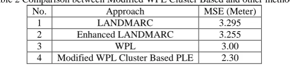
paper. The four methods were evaluated at a similar observation area. Table 2 shows the evaluation result of the four methods.

The building used for the observation was covered by a concrete wall, wooden door and window glass area of 3x43 meters

square.

Table 2Comparison between Modified WPL Cluster Based and other methods

No. Approach MSE (Meter)

1 LANDMARC 3.295

2 Enhanced LANDMARC 3.255

3 WPL 3.00

4 Modified WPL Cluster Based PLE 2.30

As shown in Table 2, the average localization accuracy, using LANDMARC, Enhanced LANDMARC, WPL and

Modified WPL Cluster Based PLE is respectively 3.295, 3.255, 3.00 and 2.30 meter. The modified LANDMARC Cluster

Based PLE enhanced the precision of localization accuracy by 29 % over LANDMARC, 28 % over Enhanced LANDMARC

and 22 % over WPL. We can conclude that the Modified WPL with Cluster-Based PLE method, as the proposed method in this

paper has the highest localization accuracy compared to the other methods in corridor A, the 3rd floor PENS Postgraduate building.

5.4. Performance Evaluation of Error Estimation Position with the Increment of Anchor Node Number

In order to evaluate the robustness of the proposed method, the error estimation position of the proposed method was

calculated by increasing the number of anchor nodes in the observation area. As shown in Fig. 4 (a) for each sub cluster, one

unknown node was kept to communicate with 3, 4 and 5 anchor nodes in the same sub-cluster. The estimated position of this

unknown node was calculated using 4 methods; furthermore, the mean square error of the estimated position will be obtained

as well. As shown in Table 3, the error performance of all approaches decreased as the density of anchor node decreased.

However, it can be observed that the localization accuracy of Modified WPL Cluster Based PLE remained in the best value

rather than the four approaches when 1 or 2 anchor nodes were removed from the test-bed location. Under this circumstance,

the modified WPL Cluster Based PLE continued to enhance the precision of localization accuracy by 24% over LANDMARC,

(11)

Based PLE continued to enhance the precision of localization accuracy by 33 % over LANDMARC, 47 % over enhanced

LANDMARC and 26 % over WPL.

Table 3 shows MSE using five anchor nodes. In this table, the MSE values of Enhanced LANDMARC, LANDMARC,

WPL and Modified WPL Cluster Based PLE were becoming smaller. An improved MSE average value was obtained by the

four anchor nodes and the three anchor nodes. But in the WPL scenario using five anchor nodes, the MSE has increased. This

condition occurred due to a similar Path Loss Exponent value of each reference node.

Table 3Comparison between Modified WPL Cluster based and other methods with the increase of anchor node numbers

No. Approach MSE (Meter)

3 Anchor Nodes 4 Anchor Nodes 5 Anchor Nodes

1 LANDMARC 3.03 3.01 3.58

2 Enhanced LANDMARC 2.9 3.16 4.55

3 WPL 3.85 2.75 3.25

4 Modified WPL Cluster Based PLE 2.08 2.28 2.40

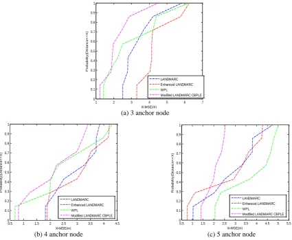
5.5. The Distribution of Mean Square Error of Estimation Position

The distribution of the four scenarios MSE i.e. LANDMARC, Enhanced LANDMARC, WPL and WPL Modified Cluster

Based PLE was analyzed using the cumulative distribution function (CDF) graph for the position error estimation of each

scenario using 3, 4 and 5 anchor nodes. CDF graph can be used to analyze the estimation error in the overall position of the data

to determine the smallest MSE value of the four scenarios tested. Figs. 5 (a), 5 (b) and 5 (c) show the graph of CDF on the

observation area using 3, 4 and 5 anchor nodes.

(a) 3 anchor node

(b) 4 anchor node (c) 5 anchor node

Fig. 5 Comparison of CDF graph of error estimation distance for different anchor node

In Fig. 5, the blue line indicates the distribution of MSE using LANDMARC scenario, the red line indicates the enhanced

LANDMARC, the green line indicates the WPL scenario and the magenta line indicates the WPL Modified Cluster Based PLE.

1 2 3 4 5 6 7

0 0.1 0.2 0.3 0.4 0.5 0.6 0.7 0.8 0.9 1 X=MSE(m) P ro b a b il it y (D is ta n c e < = X ) LANDMARC Enhanced LANDMARC WPL

Modified LANDMARC CBPLE

0.5 1 1.5 2 2.5 3 3.5 4 4.5

Modified LANDMARC CBPLE

0.5 1 1.5 2 2.5 3 3.5 4 4.5 5 5.5

(12)

As shown in Fig. 5 (c), the modified Cluster Based PLE scenario indicated by the magenta line had a range of error estimated

between 0.82 meters to 3.42 meters, while the blue line indicating the LANDMARC scenario had a range of error of estimated

between 1.82 meters to 3.85 meters, and the red line showed the enhanced LANDMARC scenario with an estimated error

ranging between 1.89 meters to 4:21 meters. In contrast to the green line that shows scenarios range of error of estimation,

WPL has a sufficient width between 0.49 to 4.31 meters. Thus, if we evaluate using the cumulative distribution function (CDF)

graph, the modified scenario WPL Cluster Based PLE had the smallest MSE value compared to the LANDMARC scenarios,

enhanced LANDMARC and WPL. Thus, we can conclude that the WPL Modified Cluster Based PLE remains more reliable

and robust when the number of anchor node has increased up to 5 anchor nodes.

5.6. Performance evaluation of the error estimation position WPL versus modified WPL cluster based PLE

According to the position accuracy of the four scenarios that has been tested, we attempted to implement the Weighted

Pathloss and modified WPL Cluster Based PLE on the observation area. The goal of the implementation is to determine the

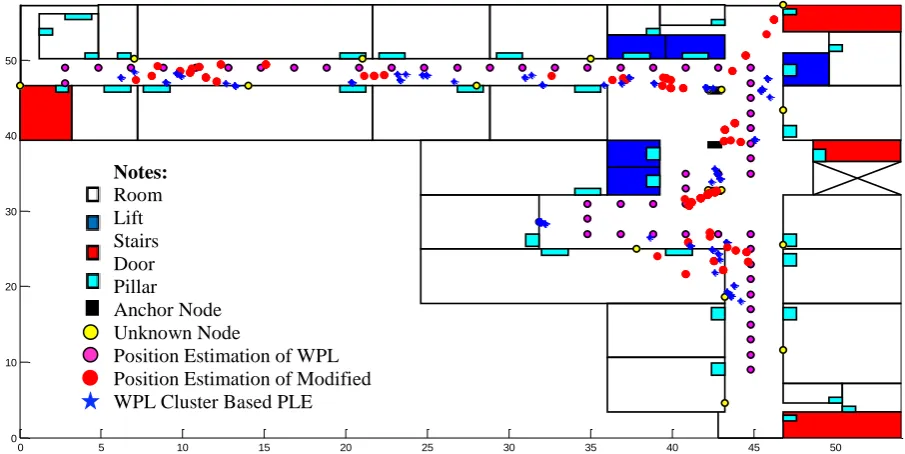
stability of the proposed method. We installed 16 pieces of anchor nodes and prepared 53 points which were assumed to be

traversed by a mobile node. Fig. 6 shows the scenario of node placement in observation area, and displays the result of position

estimation using WPL and modified WPL PLE Cluster Based on the similar area.

Fig. 6 Placement of Anchor Node, Unknown Node and the display of estimated position using WPL and proposed method

The yellow circle indicates the anchor node, the magenta circle indicates the movement of an unknown node, the red

circles indicate the estimated position of an unknown node using WPL method and the blue star indicates the estimated

position of an unknown node with modified WPL Cluster Based PLE method. Table 5 shows the mean square error of position

estimation, variance and standard deviation in an environmental observation using four methods, namely WPL with Linear

Regression PLE, Modified WPL with Linear Regression PLE, WPL with Cluster-Based PLE and Modified WPL with

Cluster-Based PLE.

12

Table 4Comparison between Modified WPL Cluster based and other methods in 3th floor of PENS Building

No. Approach MSE Estimation Position

(meter)

Variance (meter)

Standard Deviation (meter)

1. WPL using Linear Regression PLE 5.804 11.12 3.33

2. WPL using Cluster Based PLE 5.208 10.16 3.18

3. Modified WPL using Linear Regression PLE 4.00 7.7 2.78

4. Modified WPL using Cluster Based PLE 3.80 5.78 2.40

0 5 10 15 20 25 30 35 40 45 50

0 10 20 30 40 50

Notes: Room Lift Stairs Door Pillar Anchor Node Unknown Node

(13)

Table 4 shows that the modified WPL Cluster Based PLE generated the smallest MSE. According to the variance of error

position estimation, the modified WPL using Cluster Based PLE had the smallest variance value. It could be concluded that

smaller variance of error yielded a more stable method. Thus, compared to the other proposed methods, the modified WPL

cluster based PLE was the most stable in the errors.

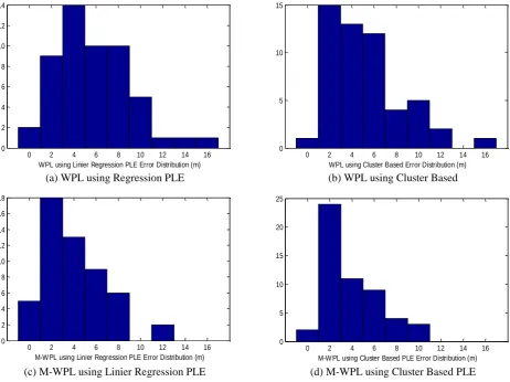
(a) WPL using Regression PLE (b) WPL using Cluster Based

(c) M-WPL using Linier Regression PLE (d) M-WPL using Cluster Based PLE

Fig. 7 Comparison of distance error distribution for various method

Fig. 7 shows the comparison of the distance error distribution for different methods. The WPL with linear regression PLE,

as shown in Fig. 7(a) has a distribution of error value larger than the other methods between 0-16 meters. This method also has

the greatest probability of error that occurred in 3 to 4 meters of position estimation. The experiment using WPL with

cluster-based PLE, as shown in Fig. 7(b) yields the same error distribution as the WPL with linear regression PLE, in the terms

of the probability that the largest error occurred in error ranges between 1 to 2 meters.

The result of experiments using the modified WPL with linear regression PLE, as shown in Fig. 7 (c) yields the

distribution of the error value which is smaller than the two previous methods, i.e. between 0-13 meters. Thus, this method able

to produce the smallest spread value compared to the other methods, where the greatest probability of error is between 1 to 2

meters. It can be concluded that the modified WPL uses Cluster Based PLE had a better performance evaluation than modified

WPL with linear regression PLE, and the modified WPL method has the capability to increase the value of accuracy better than

standard WPL position estimation method.

6. Conclusion

In this paper, a modified WPL with Cluster-based PLE method has been proposed to refine the accuracy of the estimation

position of a mobile node in an indoor environment. This method involves a profiling procedure to obtain the best performance

on estimating position technique. The variety of Path Loss Exponent due to the materials of building, furniture and the shape of

0 2 4 6 8 10 12 14 16

0 2 4 6 8 10 12 14

WPL using Linier Regression PLE Error Distribution (m)

0 2 4 6 8 10 12 14 16

0 5 10 15

WPL using Cluster Based Error Distribution (m)

0 2 4 6 8 10 12 14 16

0 2 4 6 8 10 12 14 16 18

M-W PL using Linier Regression PLE Error Distribution (m)

0 2 4 6 8 10 12 14 16

0 5 10 15 20 25

M-W PL using Cluster Based PLE Error Distribution (m)

0 2 4 6 8 10 12 14 16

0 2 4 6 8 10 12 14

0 2 4 6 8 10 12 14 16

0 5 10 15

0 2 4 6 8 10 12 14 16

0 2 4 6 8 10 12 14 16 18

0 2 4 6 8 10 12 14 16

0 5 10 15 20 25

0 2 4 6 8 10 12 14 16

0 2 4 6 8 10 12 14

0 2 4 6 8 10 12 14 16

0 5 10 15

0 2 4 6 8 10 12 14 16

0 2 4 6 8 10 12 14 16 18

0 2 4 6 8 10 12 14 16

0 5 10 15 20 25

0 2 4 6 8 10 12 14 16

0 2 4 6 8 10 12 14

0 2 4 6 8 10 12 14 16

0 5 10 15

0 2 4 6 8 10 12 14 16

0 2 4 6 8 10 12 14 16 18

0 2 4 6 8 10 12 14 16

0 5 10 15 20 25

(14)

the building will contribute to the determination of estimation distance. An experiment in different indoor environment using

the proposed methods has been conducted. The stability of the proposed methods in a different environment has been evaluated

and the proposed method has been implemented at an indoor positioning system using the wireless sensor network.

References

[1] I. T.Haque and C. Assi,“Profiling-based indoor localization schemes,”IEEE System Journal, vol. 9, no.1, pp. 76-85, 2015. [2] Z. Hengjun and Q. Hanbiao,“Research on the mine personnel localization algorithm based on the background of week

signal,”International Journal of Smart Home, vol. 10, no.7, pp. 47-56, 2016.

[3] Z. De and L. G. Yan, “Positioning system of underground coal mines based on zigbee technology,” TELKOMNIKA Indonesian Journal of Electrical Engineering and Computer Science, vol. 12, no. 5, pp. 3962-3968, 2014.

[4] W. Yan, S. Xinxin, and J. Wei, “The mobile nodes location technology in wireless sensor network,” Chinese Journal of Sensor and Actuators, vol. 24, no. 9, 2011.

[5] B. Zhou, Q. Chen, and P. Xiao, “The error propagation analysis of the received signal strength based simultaneos localization and tracking in WSN,” IEEE Transaction on Information Theory, vol. 63, pp. 3943-4007, 2017.

[6] A. A Momtaz, F. Behnia, R. Amini, and F. Marvash,“NLOS Identification in range based scene localization: Statistical Approach,” IEEE Sensor Journal, vol. 18, pp. 3745-3751, 2017.

[7] M. Singh and P.M. Khilar, “Mobile beacon based range free localization method for Wireless Sensor Networks,”Journal of Mobile Communication, Computation and Information, vol. 23, pp. 1285-1300, 2017.

[8] K. Z. Lu, X. H. Xiang, D. Zhang, R. Mao, and Y. H. Feng,”Localization algorithm based on maximum aposteriori in wireless sensor networks,” International Journal of Distributed Sensor Networks, vol. 2, no. 3, pp.198-214, 2012. [9] S. Tomic, M. Beko, R. Dinis, and P. Montezena, “Distributed algorithm for target localization in wireless sensor network

using RSS and AOA measurement,” Elsavier Journal: Pervasive and Mobile Computing, vol. 37, pp. 63-77, 2017. [10] M. Salamah and E. Doukhnitch, “An efficient algorithm for mobile objects localization,” International Journal of

Communication Systems, vol. 21, no. 3, pp. 301-310, 2008.

[11] A. Znaid, I. Idris, A. Wahab, L.K. Qabajeh, and O.A. Mahdi, “Sequential monte carlo localization method in mobile wireless sensor networks: a review,” Hindawi Journal of Sensors, vol. 1, 2017.

[12] N. U. Scholastica, “Path loss prediction model of a wireless sensor network in an indoor environment,” International Journal of Advanced Research in Electrical, Electronics and Instrumentation Engineering, vol. 4, pp. 11665-11673, 2012. [13] R. D. Ainul, P. Kristalina, and A. Sudarsono, “A. modified iterative extended kalman filter for mobile cooperative

tracking system,” International Journal of Advanced Science, Engineering and Information Technology, vol. 21, no. 3, pp. 301-310, 2016.

[14] F. Caballero, L. Merino, P. Gil, I. Maza, and A. Ollero, “A partical filter method for wireless sensor network localization with an aerial robot beacon,” Proc. 2008 IEEE International Conference on Robotics and Automation, 2014, pp. 596-601. [15] X. Chen and S. Zou, “Improve wi-fi indoor positioning based on Partical Swarm Optimization,” IEEE Sensors Journal, vol.

17, no. 21, 2017.

[16] C. R. Pratiwi, P. Kristalina, and A. Sudarsono,”Cluster based Path Loss Exponentmodel for indoor estimation distance in wireless sensor network,”Proc. The 5th International Conference on Knowledge Creation and Intelligent Computing (KCIC), IEEE Xplore, 2016, pp. 89-102.

[17] Z. Yang, Y. Liu, and X. Li, “Beyond trilateration: on the localizability of wireless Ad Hoc networks,” IEEE /ACM Transactions on Networking, vol. 18, no. 6, pp. 1806-1814, 2013.

[18] P. Kristalina, A. Sudarsono, M. Syafrudin, and B.K. Putra, “SCLoc: secure localization platform for Indoor wireless sensor network,” Proc. 2016 International Electronics Symposium, 2016, pp. 420-425.

[19] L. M. Ni, Y. Liu, Y.C. Lau, and A.P. Patil, “LANDMARC: indoor localization sensing using RFID,” Wireless Network 10, Kluwer Academic Publishers, 2004.

[20] X. Jiang, Y. Liu, and X. Wang, “An enhanced approach of indoor location sensing using active RFID,” Wase International Conference of Information Engineering, pp. 169-172, 2009.

[21] H. Zou, L. Xie, Q. S. Jia, and H. Wang, “Platform and algorithm development for a RFID-based indoor positioning System,”Journal of Unmanned Systems, vol. 2, no. 3, pp. 279-291, 2014.

[22] B.R. Jadhavar and T.R. Sontakke, “2.4 GHz propagation prediction models for indoor wireless communications within building,” International Journal Science Computer Engineering, vol. 2, no. 3, pp. 108-113, 2012.