A Quadratically Convergent
O n
(
)
Interior-Point
Algorithm for the
P*
(κ)-Matrix Horizontal
Linear Complementarity Problem
H. Mansouri
*and S. Asadi
Department of Applied Mathematics, Faculty of Mathematical Sciences, Shahrekord University, Shahrekord, Islamic Republic of Iran
Received: 14 February 2012 / Revised: 9 June 2012 / Accepted: 16 September 2012
Abstract
In this paper, we present a new path-following interior-point algorithm for
*
( )
P
κ
-horizontal linear complementarity problems (HLCPs). The algorithm uses
only full-Newton steps which has the advantage that no line searchs are needed.
Moreover, we obtain the currently best known iteration bound for the algorithm
with small-update method, namely,
O
n
(1
κ
)log
n
ε
+
, which is as good as the
linear analogue.
Keywords: Horizontal linear complementarity problem (HLCP); Interior point method (IPM); Central path
* Corresponding author, Tel.: +98(381)4421622, Fax: +98(381)4421622, E-mail: [email protected]
Introduction
Given ,Q R∈n n× and b∈n, the horizontal linear complementarity problem (HLCP) is to find a pair
2
( , )x s ∈ n such that
, ( , ) 0, T 0. ( )
Qx Rs b x s+ = ≥ x s= P
The standard (monotone) linear complementarity problem (SLCP or simply LCP) corresponds to the case where R = −I and Q is positive semidefinite.
We say that ( )P is a P∗( )κ -HLCP if 0
(1 4 ) 0, , n,
i i i i
i I i I
Qu Rv
u v u v u v
κ
+ −
∈ ∈
+ =
⇒ +
∑
+∑
≥ ∀ ∈ (1)where κ is nonnegative constant and I+=
{ :i u vi i >0} and I−={ :i u vi i <0}. If the above condition satisfied, then we say that the pair ( , )Q R is a
*( )
P κ -pair and write ( , )Q R ∈P*( )κ . For κ =0,
*( )
P κ −HLCP is called the monotone HLCP.
better choice than using any algorithm for SLCP to solve the HLCP. Close connection between LO, CQO, SLCP and HLCP cause the extension of some IPMs from LO, CQO and SLCP to HLCP. For instance, Gonzaga et al. [6, 7] studied the largest step path following algorithm for monotone HLCP and showed the fast convergence of the simplified path following algorithm. Mizuno et al. [8] proposed the (MTY) predictor-corrector method that was the first polynomial-time and superlinear convergent IPM for general LO, with precisely O
( )
nL iteration complexity.(cf. [8]). The MTY method generalized to SLCP in [9] and the resulting algorithm has O( )
nL iterations. Also in [10] the MTY method has been generalized to HLCP and a class of corrector-predictor IPMs for solving P*( )κ -HLCP has been proposedtherein. Huang [11] proposed a high-order feasible interior-point method for HLCP with O nlogε0
ε
iterations. Monteiro et al. [12] studied the limiting behavior of the derivatives of certain trajectories associated with the monotone HLCP. Some other relevant references can be found in [13, 14]. It should be noted that all most known polynomial various of IPMs used the so-called central path as a guideline to the optimal set, and some various of the Newton method to follow the central path approximately. However there is still a gap between the practical behavior of these algorithms and the theoretical performance results with respect to the update strategies of the duality gap parameter in the algorithm. The so-called large-update IPMs have superior practical performance but with relatively weak theoretical results. While the so-called small-update IPMs enjoy the best known worst-case iteration bound but their performance in computational practice is poor. This gap was reduced by Peng et al. [15] who introduced the so-called self-regular barrier functions based on IPMs for LO and semidefinite optimization (SDO). See also Salahi et al. [16]. Bai et al. [17] and Amini et al. [18] who presented IPMs based on a new class of non-self-regular kernel functions for LO and P*( )κ -linear complementarity problems and also obtained the same best known iteration bounds for the algorithms with large- and small-update methods as they are in [15]. In very recently, Mansouri et al. [19-21] presented the first full-Newton step IPM for Linear Complementarity problems (LCPs) and P∗( )κ -HLCPs, which are an extension of the work for linear optimization [22-24].
In this paper we present a new feasible primal-dual
IPM with full-Newton steps for HLCP problems. We prove that the complexity of our algorithm is
(1 )logn
O n
κ
ε
+
iteration, which coincides with the
best known iteration bound for feasible IPMs .
The notations used throughout the paper is rather standard: capital letters denote matrices, lower case letters denote vectors, script capital letters denote sets, and Greek letters denote scalars. All vectors are considered to be column vectors. The components of a vector u∈n will be denoted by , 1, ,
i
u i = n. The relation u>0 is equivalent to ui >0,i =1, , n, while
0
u≥ means ui ≥0,i =1, , n. We denote
{ : 0}
n u n u
+ = ∈ ≥
and n {u n:u 0}
++ = ∈ >
. If
n
u∈ , then U diag u= ( ) denotes the diagonal matrix having the components of u as its diagonal entries. If
, n
x s∈ , then xs denotes the componentwise (Hadamard) product of the vectors x and s. Furthermore, e denotes the all-one vector of length n. The 2-norm and the infinity norm for vectors are denoted by and ∞, respectively. We denote the set of feasible points of the HLCP by
2
{( , ) n: },
F = x s ∈+ Qx Rs b+ = (2)
and the set of strictly feasible (or interior) points by
0 {( , ) 2n : },
F = x s ∈++ Qx Rs b+ = (3)
and the solution set of HLCP by
* {( , )* * : * * 0}.
F = x s ∈F x s = (4) Throughout this paper it is assumed that F* is not
empty, i.e. ( )P has at least one solution.
Materials and Methods
1. Feasible Full Newton Step IPMs and Central Path
Solving HLCP is equivalent with finding a solution of the following system of equations:
, 0,
0, 0,
Qx Rs b x
xs s
+ = ≥
= ≥ (5)
where the first constraint represents feasibility and the second is the so-called complementarity condition.
system:
, 0,
, 0,
Qx Rs b x
xs µe s
+ = ≥
= ≥ (6)
In [25] it has been shown that if HLCP satisfies the interior-point condition i.e. there exists ( , ) 0x s > such that Qx Rs b+ = , then the above system has a unique solution for each
µ
>0. Denote this unique solution by ( ( ), ( ))x µ s µ , for everyµ
>0. Then we call ( ( ), ( ))x µ s µ the µ−center of HLCP. The set of µ−centers (with µ running through all positive real numbers) gives a homotype path, which is called the central path of HLCP. If
µ
→0, then the limit of the central path exists [25] and it yields the optimal solution for HLCP.2. Definition and Properties of the Newton Step
IPMs follow the central path approximately. Let us describe how this proceeds. A direct application of Newton’s method to solve the system (6) with fixed μ, and assuming ( , ) 0x s > , produces the following system for the displacement ∆x and ∆s:
( ) ( ) ,
( )( ) .
Q x x R s s b
x x s s µe
+ ∆ + + ∆ =
+ ∆ + ∆ =
By omitting the quadratic term ∆ ∆x s in the second equation, we have the following linear system of equations:
( ),
. Q x R s b Qx Rs
s x x s µe xs
∆ + ∆ = − +
∆ + ∆ = −
Note that if ( , )x s is a feasible solution of HLCP, then Qx Rs b+ = . Hence, the above system reduces to
0, . Q x R s
s x x s µe xs
∆ + ∆ =
∆ + ∆ = − (7)
The new iterates are given by ,
.
x x x s s s
+
+
= + ∆
= + ∆
3. Proximity Measure
In the case of a feasible method we call the ( , )x s
an ε−solution of HLCP if x sT ≤
ε
. To measure thequality of any approximation ( , )x s of ( ( ), ( ))x µ s µ , we introduce δ( , ; )x s µ that vanishes if
( , ) ( ( ), ( ))x s = x µ s µ and is positive otherwise. To this end we introduce the variance vector of ( , )x s with respect to µ as follows
, xs
v = µ
where all operations are componentwise. Note that .
xs =µe⇔ =v e
The proximity meature δ( , ; )x s µ is now defined by
1
1
( , ; ) ,
2
x s v v
δ
µ
= − − (8)Note that if ( , ) ( ( ), ( )),x s = x µ s µ then v e= and hence δ( , ; ) 0x s µ = and otherwise δ( , ; ) 0x s µ > .
Results
1. Feasibility and Quadratic Convergence of the Feasible Full-Newton Step
In this section we find a condition for feasibility of full Newton steps. We also prove that the value of x sT after one step is less than or equal to
(
n+δ µ2)
. Wealso prove that the full Newton steps are quadratically convergent to the target point ( ( ), ( ))x µ s µ . Define
1 1
, , , ,
x v x s v s
d d Q QV X R RV S x s
− −
∆ ∆
= = = = (9)
where X =diag x S diag s( ), = ( ) and V =diag v( ). Now we can easily check that the system (7), which defines the search directions ∆x and ∆s, can be expressed in terms of the scaled search directions dx and ds as follows:
1
0, .
x s
x s
Qd Rd d d v− v
+ =
+ = − (10)
Now, using (9) and the second equation in (7), we have
( )( )
2
( )
( ).
x s x s
xs x s s x x s e x s
xs
e d d e d d
v
µ
µ µ
= + ∆ + ∆ + ∆ ∆ = + ∆ ∆
= + = +
Lemma 1.1 (Cf. Lemma II.45 in [1]) The new iterates ( , )x s+ + are strictly feasible if and only if
x s e d d+ > 0. Proof: Note that if x+ and s+ are positive, then the
above equality makes clear that e d d+ x s> 0, proving the ’only if ’ part of the statement in the lemma. For the proof of the converse implication, we introduce a step length
α
∈[0,1], and we define, .
xα = + ∆x α x sα = + ∆s α s
We then have x0 =x x, 1=x+ and similar relations
for .s Hence we have x s0 0=xs >0. We may write
2
( )( )
( )
x s x x s s
xs s x x s x s
α α α α
α α
= + ∆ + ∆
= + ∆ + ∆ + ∆ ∆ . Using s x x s∆ + ∆ =
µ
e xs− gives2
( )
x sα α =xs+α µe xs− +α ∆ ∆x s.
Now suppose that e d d+ x s >0. From the definitions of dx and ds in (9) we deduce that µd dx s = ∆ ∆x s. Hence
µ
e+ ∆ ∆ >x s 0, or, equivalently,x s
µ
e∆ ∆ > − . Substitution gives
2
( ) (1 )( )
x sα α>xs+α µe xs− −α µe= −α xs+α µe ,
[0,1]
α
∈ .Since (1−α)(xs+α µe) 0≥ , it follows that 0
x sα α > , for all 0≤ ≤α 1. Hence, none of the entries
of xα and sα vanishes for 0≤ ≤α 1. Since x0 and s0
are positive, and xα and sα depend linearly on α, this
implies that xα >0 and sα >0 , for all 0≤ ≤α 1.
Hence, x1 and s1 must be positive which proves that
x+ and s+ are positive. □
Corollary 1.2 The iterates ( , )x s+ + are strictly feasible
if d dx s ∞ <1.
Proof: By Lemma 1.1, x+ and s+ are strictly feasible
if and only if e d d+ x s >0. Since the last inequality holds if d dx s ∞ <1, then the corollary follows. □
The following lemma gives some bounds for the solution of a linear system of the form:
, 0.
+ =
+ =
su xv a
Qu Rv (11)
Using the notations
1 1 1
2 2, ( ) ,2
D X S= − a= xs a−
where X =diag x( ) and S diag s= ( ), we have the following result.
Lemma 1.3 Let ( , )Q R in the HLCP be a P∗( )κ -pair. Then for any ( , )x s 2n
++
∈ and a∈n, the linear
system (11) has a unique solution ( , )u v , for which the following estimates hold
2 1 2 1 2
, .
4 8
T
a u v a uv a
κ κ
− ≤ ≤ ≤ +
Proof: We consider the index sets:
{ : i i 0}, { : i i 0}.
I+= i u v > I−= i u v <
Using the relations
1 2 2
0 4< u vi i ≤(Du D v− − )i =ai , ∀ ∈i I+,
2
1
(1 4 ) ,
4
i i i i
i I i I
u v κ u v κ a
− +
∈ ∈
≤ + ≤ +
∑
∑
where we use this fact that ( , )Q R is a P∗( )κ -pair, we deduce that
2
1 .
4 T
i i i i i i
i I i I i I
u v u v u v u v a
+ − +
∈ ∈ ∈
=
∑
+∑
≤∑
≤ Also we have
2
(1 4 ) 4
4 .
T
i i i i
i I i I
i i i i i i
i I i I i I
i i i I
u v u v u v
u v u v u v u v a
κ κ
κ κ
+ −
+ − +
+
∈ ∈
∈ ∈ ∈
∈
= +
= + + −
≥ − ≥ −
∑
∑
∑
∑
∑
∑
This proves the first inequality in the lemma. For the second inequality we have
2 2 2 2 2 4
2 2
4 4
1 16
1 1
16 4
i i i i i
i I i I i I
i i i I
uv u v u v a
u v a κ a
+ − +
−
∈ ∈ ∈
∈
= + ≤
+ ≤ + +
∑
∑
∑
∑
2
4 4
2
1 1 .
8 2κ κ a 8 κ a
= + + ≤ +
-pair. Then the unique solution ( ,∆ ∆x s) of the system (7) satisfies the following inequalities:
2 2
2 ( ) ,
2 T
x s µδ
µκδ
− ≤ ∆ ∆ ≤ (12)
2
1
2 .
8
x s κ µδ
∆ ∆ ≤ +
(13)
Proof: It suffices that we apply Lemma 1.3 with a=µe xs− and ( ,∆ ∆x s) instead of ( , )u v and note that
1
1 ( )
( ),
e a e xs xs
xs xs
xs v v xs
µ µ
µ
µ µ
µ
−
= − = −
= − = −
which implies
2
2 1 2 2,
a =µ v− −v = µδ
that completes the proof. □ Lemma 1.5 After a Newton step one has
2
( )x+ Ts+≤(n+δ µ) .
Proof: By using x+= + ∆x x and s+ = + ∆s s , after a
Newton step one has
2 2
( ) ( ) (( )( ))
( )
( ) ( ) ,
T T T
T
T
x s e x s e x x s s e xs x s s x x s
e µe x s nµ µδ n δ µ
+ + = + + = + ∆ + ∆
= + ∆ + ∆ + ∆ ∆
= + ∆ ∆ ≤ + = +
where the inequality follows because of (12). This completes the proof. □
Lemma 1.6 Let δ+ =δ( , ; )x s+ + µ . Then 2
2
1 2 2 2
. 1 2 2 1
2
κ δ δ
κ δ
+
+
≤
+
−
Proof: Let v+ be the variance vector of ( , )x s+ + with
respect to µ, i.e. v+= x sµ+ + , then we have
(
)
1 1 2
2δ+ = ( )v+ − −v+ = ( )v+ − e v−( ) .+
Since x s+ += +∆ ∆µe x s , we obtain ( )v 2 e x s
µ
+ = +∆ ∆ .
Then
2 .
1 x s x s
x s x s
e
µ µ
δ
µ µ
+
∞
∆ ∆ ∆ ∆
−
= ≤
∆ ∆ ∆ ∆
+ −
Using (13) and the fact that ∆ ∆x s ∞≤ ∆ ∆x s , we have
2
2
1 2
8
2 ,
1 1 2
8
κ δ δ
κ δ
+
+
≤
− +
which completes the proof. □ Corollary 1.7 If
(
1)
( , ; )
2 1 2 2 x s
δ δ
µ
κ
= ≤
+ then
we have
(
)
2( , ; )x s 1 2 2 ,
δ+ =δ + + µ ≤ + κ δ
i.e. quadratic convergence to the µ-center is obtained.
2. Updating the Barrier Parameter μ
In this section, we obtain a simple relation for our proximity measure just before and after a µ-update. Lemma 2.1 Let ( , )x s be a positive pair and
µ
>0 is such that x sT ≤(n+δ µ2) . Moreover, let( , ; )x s
δ δ= µ and µ+= −(1 θ µ) . Then, one has
2 2
2 2
( , ; ) (1 ) .
2(1 ) 2(1 )
n
x s θ δ
δ µ θ δ
θ θ
+ ≤ − + +
− −
Proof: Assume that δ+=δ( , ;x s µ+), then we have
2
2 1
2 1
2( ) 1
1
1 ( )
1 v v
v
v v
δ θ
θ
θ θ
θ
+ −
−
= − −
−
= − − −
−
2
2 2
1 1
(1 ) 2 ( ).
1 T
v v
θ
v v v vθ
θ
θ
− −
= − − + − −
−
Since x sT ≤(n+δ µ2) we obtain that v 2≤ +n δ2.
(
)
(
)
2
2 2 2 2
2( ) 2(1 ) 2 2
1 n n n
θ
δ
θ δ
δ
θ θ
δ
θ
+ ≤ − + + − + + − 2 2 2 22(1 ) 2
1 1
nθ θ
θ δ θ δ
θ θ = − + + + − − 2 2
2 2 2
2(1 )
1 1
nθ θ θ
θ δ δ
θ θ − = − + + − − 2 2
2 1 ( 1) 2
2(1 )
1 1
nθ θ
θ δ δ
θ θ − − = − + + − − 2
2 1 2
2(1 ) .
1 1
n
θ
θ δ
δ
θ
θ
≤ − + +
− −
It completes the proof. □
3. Complexity Analysis
In this subsection we present a lemma that gives the complexity of the algorithm. At the start of the algorithm, we have a point ( , )x s that is strictly feasible for ( )P and a
µ
>0 such that(
1)
( , ; )
2 1 2 2 x s
δ µ τ
κ ≤ =
+ . Then, after the barrier
parameter is updated to µ+ = −(1 θ µ) , with
(
1 2 21)
8n,θ
κ =
+ Lemma 2.1, yields the following
upper bound for ( , ;δ x s µ+):
(
)
(
)
(
)
(
)
(
)
(
)
2 2 2 2 2 2 2 1 ( , ; )4 1 2 2 1 16(1 ) 1 2 2
1 8(1 ) 1 2 2
1 3
4 1 2 2 16(1 ) 1 2 2
1 .
2 1 2 2
x s θ
δ µ
κ
θ κ
θ κ
θ
κ θ κ
κ + ≤ − + + − + + − + − = + + − + ≤ +
Assuming n≥2, The last inequality follows since its left hand side is a convex function of ,θ whose value
is
(
)
27
16 1 2 2+ κ both in θ =0 and
(
)
1 4 1 2 2
θ
κ =
+ .
Since
(
1)
0, ,
4 1 2 2
θ κ ∈ +
the left hand side does not
exceed
(
)
27
16 1 2 2+ κ .Since
(
) (
2)
27 1
16 1 2 2+ κ <2 1 2 2+ κ ,
it follows that after the µ−update we have
(
)
2 2
2
1 ( , ; )
2 1 2 2
x s
δ δ µ
κ
+
= ≤
+ . Thus, by Corollary 1.7, after performing the Newton step we certainly have
(
)
(
)
(
)
(
)
2
2
( , ; ) 1 2 2
1 1
1 2 2 ,
2 1 2 2 2 1 2 2
x s
δ µ κ δ
κ τ κ κ + + + ≤ + ≤ + ≤ = + +
therefore the algorithm is well defined. The above explanation implies the following result which establishes the polynomial iteration complexity of the algorithm.
Theorem 3.1 If
(
1 2 21)
8nθ
κ =
+ , the number of
iterations of the feasible primal-dual path-following algorithm with full-Newton steps does not exceed
(
)
08 1 2 2 logn
κ
nµ
.ε
+
4. Numerical Results
In this section we present some numerical results. We solve the following P*(0) (monotone) linear complementarity problems, so R = -I, using the algorithm in Figure 1. The initialization parameters are assumed as described in Section 3, and the accuracy parameter ε is set to 10−4 and τ =0.5. Tables 1-4
show the number of iterations to obtain ε-solutions of the problems with the algorithm.
Problem 4.1
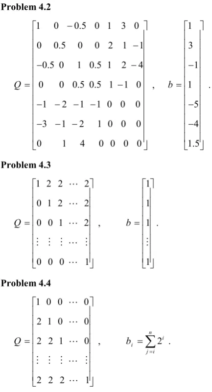
Problem 4.2
1 0 0.5 0 1 3 0
0 0.5 0 0 2 1 1 0.5 0 1 0.5 1 2 4
0 0 0.5 0.5 1 1 0
1 2 1 1 0 0 0
3 1 2 1 0 0 0
0 1 4 0 0 0 0
Q
−
−
− −
= −
− − − −
− − −
, 1 3 1 1
5 4 1.5 b
− =
− −
.
Problem 4.3
1 2 2 2
0 1 2 2
0 0 1 2
0 0 0 1
Q
=
, 1 1 1
1 b
=
.
Problem 4.4
1 0 0 0
2 1 0 0
2 2 1 0
2 2 2 1
Q
=
, n 2i i
j i b
=
=
∑
.Problems 4.3 and 4.4 are all known to have exponential complexity for pivoting methods, but our results show slow growth as n increases, which is precisely what is hoped for interior-point methods.
5. Concluding Remarks and Further Research
We have presented an interior-point algorithm for HLCPs. At each iteration, we use only full-Newton steps. The favorable polynomial complexity bound for the algorithm with the small-update method is deserved, namely, O n(1
κ
)lognε
+
. Moreover, the resulting
analysis is relatively simple and straightforward to the LO analogue.It may be clear that this full-Newton step method, may not be efficient in practice, Just as almost all feasible IPMs with the best theoretical performance. But this gap between the practical and theoretical performance can be reduced with changing the search
direction by using methods that are based on kernel functions, as presented in [3, 16, 18, 27]. We leave it to the future to analyze a full-Newton step method based on kernel functions.
Feasible IPM for P*( )κ -HLCP Input:
Accuracy parameter ε >0; threshold parameter τ<1;
barrier update parameter θ, 0< <θ 1;
feasible pair ( , )x s0 0 with ( )x0 Ts0=nµ0 and
0 0
µ > such that δ( , ; )x s0 0 µ0 ≤τ.
begin
x:=x0; :s =s0; :µ =µ0;
while n
µ ε
≥ do beginupdate of µ: µ: (1= −θ µ) ;
( , ) : ( , ) ( , );x s = x s + ∆ ∆x s end
end
Figure 1. Feasible full-Newton-step algorithm.
Table 1. The number of iterations for problem 4.1
θ Iterations (x*)T
0.17 56 [0.09,0.99,1.72,0.38]
Table 2. The number of iterations for problem 4.2
θ Iterations (x*)T
0.13 79 [0.1,0,0.3,0,0.7,0.16,0.33]
Table 3. The number of iterations for problem 4.3
n θ Iterations (S*)T
10 0.11 99 [0,0,…,0.09]
20 0.08 150 [0,0,…,0.05]
30 0.06 191 [0,0,…,0.03]
Table 4. The number of iterations for problem 4.4
n θ Iterations (S*)T
10 0.11 89 [0,0,…,0.23]
20 0.08 136 [0,0,…,0.23]
Acknowledgements
Authors wish to thank two anonymous referees for useful comments and suggestions on an earlier draft of the manuscript. The authors would like to thank for the financial grant from Shahrekord University.
References
1.Roos, C., Terlaky T. and Vial J.-Ph. Theory and Algorithms for Linear Optimization: An Interior-Point Approach, John Wiley & Sons, Chichester, UK, (1997) (2nd Edition, Springer, 2006).
2.Ai, W. B. and Zhang, S. Z. An O( n L) iteration primal-dual path-following method, based on wide neighborhoods and large updates, for monotone linear complementarity problems. SIAM J. Optim. 16 (2): 400- 417 (2005). 3.Peyghami, M. R. and Amini, K. Kernel function based
interior-point methods for solving P*(κ)-Linear
Complementarity Problem, Acta Mathematica Sinica
26(9): 1761-1778 (2010).
4.Potra, F. A. and Wright, S. J. Interior-point methods. J. Comput. Appl. Math. 124(1-2): 281-302 (2000).
5.Anitescu, M., Lesaja, G. and Potra, F. A. Equivalence between different formulations of the linear complementarity problem. Optim. Method Softw. 7(3): 265-290 (1997).
6.Gonzaga, C. and Bonnans, J. Fast convergence of the simplified largest step path following algorithm. Math. Program. 76: 95-115 (1997).
7.Gonzaga, C. The largest step path following algorithm for monotone linear complementarity problems. Math. Program., 76: 309-332 (1997).
8.Mizuno, S., Todd, M. J. and Ye, Y. On adaptive-step primal-dual interiorpoint algorithms for linear programming. Math. Oper. Res. 18(4): 964-981 (1993). 9.Miao, J.A quadratically convergent O((1+κ) n L
)-iteration algorithm for the P*(κ)-matrix linear
comple-mentarity problem. Math. Program. 69: 355–368 (1995). 10.Gurtuna, F., Petra, C., Potra, F. A., Shevehenko, O. and
Vancea, A. Corrector-Predictor methods for sufficient linear complementarity problems. Compute. Optim. Appl.
48: 453-485 (2011).
11.Huang, Z. H. Polynomiality of high-order feasible interior point method for solving the horizontal linear complementarity problems. J. System Sci. Math. Sci.
20(4): 432-438 (2000)
.
12.Monteiro, R. and Tsuchiya, T. Limiting behavior of the derivatives of certain trajectories associated with a monotone horizontal linear complementarity problem. Math. Oper. Research. 21(4): 793-814 (1996).
13.Xiu , N. H. and Zhang, J. Z. A smoothing Gauss-Newton
method for the generalized HLCP. J. Comput. Appl. Math.
129: 195-208 (2001).
14.Ma, C. F. and Chen, X. H. The convergence of a one-step smoothing Newton method for P0-NCP based on a new
smoothing NCP-function. J. Comput. Appl. Math. 216 (1): 1-13 (2008).
15.Peng, J., Roos, C. and Terlaky, T. Self-regular functions and new search directions for linear and semidefinite optimization. Math. Program. 93: 129-171 (2002). 16.Salahi, M., Terlaky, T. and Zhang G. The complexity of
self-regular proximity based infeasible IPMs. Computational Optimization and Applications 33(2): 157-185 (2006).
17.Bai, Y. Q., Ghami, M. El. and Roos, C. A comparative study of kernel functions for primal-dual interior-point algorithms in linear optimization. SIAM J. Optim. 15 (1): 101-128 (2004).
18.Amini, K. and Peyghami, M. R. Exploring complexity of large update interior-point methods for P*(κ)-linear
complementarity problem based on Kernel function. Applied Mathematics and Computation 207: 501-513 (2009).
19.Mansouri, H., Zangiabadi, M. and Pirhaji, M. A full-Newton step O(n) infeasible interior-point algorithm for linear complementarity problems. Nonlinear Anal. Real World Appl. 12: 545-561 (2011).
20.Zangiabadi, M. and Mansouri, H. Improved infeasible-interior-point algorithm for linear complementarity problems. Bulletin Iranian Math. Soc. inpress (2011). 21.Asadi, S. and Mansouri, H. Polynomial interior-point
algorithm for P*(K) horizontal linear complementarity
problems. Numerical Algorithms DOI 10.1007/s11075-012-9628-0.
22.Mansouri, H. and Roos, C. Simplified O(n) infeasible interior-point algorithm for linear optimization using full-Newton step. Optim. Methods and Soft. 22(3): 519-530 (2007).
23.Mansouri, H. Full-Newton step interior-point methods for conic optimization. Ph.D. thesis, Faculty of Mathematics and Computer Science, TUDelft, NL--2628~CD~Delft, The Netherlands (2008).
24.Roos, C. A full-Newton Step O(n) Infeasible Interior-Point Algorithm for Linear Optimization. SIAM J. Optim.
16(4): 1110-1136 (2006).
25.Stoer, J. and Wechs, M. Infeasible-interior-point paths for sufficient linear complementarity problems and their analyticity. Math. Program. Ser. A 83(3): 407-423 (1998). 26.Kojima, M., Megiddo, N., Noma, T. and Yoshise, A. A
unified approach to interior point algorithms for linear complementarity problems. Lecture Notes in Comput. Sci. vol. 538. Springer, New York, (1991).
27.Wang, G. Q. and Bai, Y. Q. Polynomial interior-point algorithms for P*(κ) horizontal linear complementarity