Singular Integral Equations in Electromagnetic Waves Reflection Modeling

www.astesj.com 82

Singular Integral Equations in Electromagnetic Waves Reflection Modeling

A. S. Ilinskiy1_{, T. N. Galishnikova}*,1

1 _{Faculty of Computational Mathematics and Cybernetics, Lomonosov Moscow State University, 119991, Russia}

A R T I C L E I N F O A B S T R A C T

Article history:

Received: 01 March, 2017 Accepted: 29 March, 2017 Online: 11 April, 2017

The processes of reflection of three-dimensional electromagnetic waves by locally irregular media interfaces are investigated. The problem under study is mathematically reduced to the solution of a boundary value problem for the Maxwell equations in an infinite space with an irregular boundary. In order to develop a numerical algorithm, the potential theory and a special Green’s function are applied to reduce the addressed boundary problem to an equivalent system of two hypersingular integral equations. This system is solved with the use of the approximation and collocation method. Special attention is focused on calculation of the kernels of these equations. Results of simulation of the currents induced on the irregularity and reflected field patterns in the resonance frequency range are presented.

Keywords:

Reflection of electromagnetic waves

Inhomogeneous medium Singular integral equations

1. Introduction

This paper is an extension of the work originally presented at the URSI Commission B International Symposium on Electromagnetic Theory (EMTS 2016) [1]. In this article we model the scattering of three-dimensional electromagnetic waves on a finite impedance section of a wavy surface separating two media. The scattering of electromagnetic waves by a wavy interface between two different media is an important problem for various applications. In this article we investigate the incidence of an arbitrary plane wave on a local inhomogeneity of the interface assuming sufficiently high conductivity of the underlying medium. The mathematical formulation of such problems reduces to that of solving a system of Maxwell equations in non-regular infinite regions. Depending on the polarization of the incident field, the boundary-value problems are reduced to independent systems of hypersingular integral equations solved by specially developed numerical algorithms utilizing a singularity isolating algorithm.

2. Mathematical model and numerical algorithm

2.1.Mathematical formulation of wave scattering problems

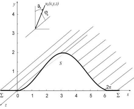
Let us assume that an interface between two media is situated in Cartesian coordinates x, y, z. The interface consists of two half planes



that are specified by the equation y0 and joined by an impedance cylindrical wavy section S that stretches along the z axis. The entire wavy section is located in the half-space

. 0



y The surface S is specified by the equation y=f(x),

,

0xa f(0) f(a)0, where ais the x length of irregularity S. Let

a



2



.

The reflecting surface

S





does not depend on z coordinate. Denote by D₁ the region over interface

S





where the 3D incident electromagnetic field propagates. This region D₁ is characterized by permittivity ₁, permeability ₁, and the k₁ wave number 1 1

2 2

1   

k , where



is the circular frequency (Figure 1). The time dependence is exp



it



.

Figure 1:Geometry of perfecting surface

ASTESJ

ISSN: 2415-6698

*_{Corresponding Author: T. N. Galishnikova, Faculty CMC,LomonosovMoscow}

State University, 119991, Russia. Email: [email protected]

www.astesj.com

Special Issue on Recent Advances in Engineering Systems

A. S. Ilinskiyet. al. / Advances in Science, Technology and Engineering Systems Journal Vol. 2, No. 3, 82-87 (2017)

The field of the plane wave

), exp( ) , , ( ), exp( ) , , ( 0 0 0 0 0 0 0 0 0 0 z i y i x i H z y x H z i y i x i E z y x E                 0 0 1

0 sin



sin





k



₀ k₁cos



₀sin



₀, and ₀k₁cos₀

is incident on the surface

S





in region D1. Here,



0 is the

angle between axis z and the direction of the incident wave propagation. When



₀ 



/2, we obtain a plane reflection two-dimensional problem. If ₀ 0, we have the case of the normal incidence in the plane problem.

In region

D

₁ we seek for a solution to the homogeneous system of Maxwell equations

, 0 ) , , ( ) , , ( , 0 ) , , ( ) , , ( 1 1           z y x H i z y x E curl z y x E i z y x H curl  

which satisfies on the plane section  the condition of perfect conduction



nE(x,y,z)



0,

Leontovich condition on local section S with a finite conductance



nE(x,y,z)



W₂



n



nH(x,y,z)





, .

/ ₂

2

2  

W Here, ₂ and ₂ are the characteristics of the section S, n



n_x,n_y,0



is the outward normal to region D₁. The reflected field satisfies the radiation conditions at infinity.

We look for the total electromagnetic field in D1 that has the

same dependence on z as the incident field, that is



x,y,z

  

E x,y exp



i ₀z



,

E    H



x,y,z



H

 

x,y exp



i₀z



. Then, the boundary condition on S can be represented as follows:

 

 

 

 

_

_

 

 

                                    y x E i n y x H i k W y x H n y x E i y x H i k W y x E z z z z z z , , 1 , , , , 0 1 2 0 2 1 2 1 0 2 0 2 1 2

,

, / /

/nn_x xn_y y

 /



n_x/yn_y/x are

the normal and tangent derivatives, respectively. Accordingly, boundary conditions on plane section



take the form

 

, 0,

 

, 0.

   n y x H y x

Ez z

We denote u

 

x,y Ez

 

x,y ,

v

 

x

,

y



H

z

 

x

,

y

,

. 2 0 2 1 2 1 

 k  Then the considered boundary value problem can

be reduced to solving in region D1 of the 2D homogeneous

Helmholtz wave equation

0 ) , ( ) , ( 2 1 2 2 2 2                      y x v y x u y x 

with appropriate boundary conditions on



and

S

.

2.2.Reduction of the boundary problem for Helmholtz equations to the system of singular equations in case of E-polarization

In order to obtain a system of hypersingular integral equations equivalent to the boundary value problem for Helmholtz equation, we introduce Green’s function gE



M,P



, satisfying in region

1

D the inhomogeneous Helmholtz equation



,



2



,



,

2 1 2 2 2 2 P M P M g y x

E _

 _             

the boundary condition for perfect conductor on half-plane





M,P



0, gE

that have the form











ˆ



.

2 ) ,

( ₀(1) _{1 M,P 0}(1) _{1 M,Pˆ} E r H r H i P M

g     

Here, H₀(1)(x) is the zero-order Hankel function of the first kind;



 

2



2,

,P M P M P

M x x y y

r     where



xM,P,yM,P



are

coordinates of M and P points; 

P M

rˆ _,ˆ



x_M x_P

 

2  y_M y_P



2,





x

P

,



y

P



are the coordinates

of the Pˆ point.

Applying in region

D

₁ the Green’s formula successively to functions u

 

M , gE



M,P



, taking into account the radiation conditions and the properties of surface potentials, we obtain a system of two integral equations for unknown functions

 

P n

u 

 / and v

 

P / on finite section S for E- polarization case:       M M M v W i n M u W W ik









) ( 2 ) (

2 ₁2

2 0 2 1 1 2 1                  



_P S P E E n P u n P M g W W ik P M

g ( , ) ( , ) ( )

2 1 2 1 1 2 1





(1)

), ( ) ( ) , ( 0 2 2

0 v P _{ds u M}

A. S. Ilinskiyet. al. / Advances in Science, Technology and Engineering Systems Journal Vol. 2, No. 3, 82-87 (2017)

 

_

  

  

    

  

   

  

 



_P

S M P

E

M E

M n

P u n n

P M g W

W ik n

P M g n

M

u ( , ) ( , ) ( )

2 1 2

1 2

2 1 1

2 1





, , ) ( )

( ) ,

( 0

2

2 1 2

0 _{M S}

n M u ds P v n n

P M g W i

M E

P P P M E

 

          

 



(2)

where u₀E(x,y)exp



i₀xi₀y



exp



i₀xi₀y



. In the case of the H- polarization we can obtain a system of two integral equations for unknown functions v

 

P and u

 

P / on finite section S.

2.3.The numerical algorithm for the solution of singular integral equations for the E-polarization

The systems of integral equations are singular and can be solved through reducing them to the complex system of linear algebraic equation by means of the collocation and approximation method.

To this end, we divide the interval

 

0,a, on which the equation y f(x) of the irregular cylindrical surface

S

is defined, by points x_i ia/N, x₀ 0, x_N a, into

N

equal parts. The points dividing the curve

S

have the coordinates



x_i,f(x_i)



. Then we replace the integrals entering into the systems of equations (1), (2) with the sums of the integrals over

the subintervals and set ,

2 1  Mi

M i1,...,N, 2 1  i

M are

collocation points. The sought solution on the section

,

1

, j

jP

P

S

, 1 ,...,

0 

 N

j is approximated by a zero-order spline. As a result, we obtain a complex system of linear algebraic equations. When calculating the integrals over a section

,

1

, j

jP

P

S

in which

the integrand depends on either gE



M,P



or



,



, P E

n P M g

 

we

replace the integration with respect to

s

with the integration with respect to

x

by setting ds_P 1



f

 

x



2dx_P.

Note that the terms that enter the kernels of integral equations and depend on gE(M,P) have a logarithmic singularity when the arguments coincide. Therefore, when developing the numerical algorithm, this singularity is separated in an explicit form and the integrals containing it are calculated analytically.

The normal derivatives of the function gE(M,P) have no singularity when the arguments are equal, and

), ( 2 1 ) , (

lim 0 M

n P M g

p E

M P

  

 

where



₀(M)is the curvature of the contour

S

at the point

M

.

The kernels of the system depending on





P M

E

n n

P M g

 

2 ,

have a strong singularity. In order to calculate the matrix elements that are integrals of the functions with a hypersingularity, it is necessary to develop a numerical algorithm. To this end, we preserve the integration over the arc

s

in these integrals. We defined the surface

S

in the form xx

 

s, yy

 

s . The outward normal to the domain D₁ we write in the form ny_six_s j, where

i



and



j

are the

x

and

y

unit vectors. Note that if the boundary of S is specified in the form y f

 

x , the relationship between the directional cosines

n

_x

;

n

_y of the outer normal n to D₁ is given by

 





2

1 f x

n

y_S  _x   , x_S n_y 1



f

 

x



2 ,

 



 



2

1

/ f x

x f

n_x     , n_y 1/ 1



f

 

x



2 .

We have







 









1 ,

,

2 / 1 2

j P j P

S

P i

E

P M

ds P M g n n

(3)







 









1 ,

2 / 1 ,

1 ) 1 ( 0 2

2 j P j P

i

S

P P M P

M

ds r

H n n

i _









 

 

1 ,

2 /

1 .

ˆ

2 1 ,

) 1 ( 0 2

j P j P

i

S

P P M P

M

ds r

H n n

i _

To develop a special computing algorithm, every integrands is represented by a sum of two terms: the first one is the total differential of some function has been calculated analytically; the function in the second term has a logarithmic singularity and is integrated by separating this singularity in the explicit form, thereafter the corresponding integrals are calculated analytically.

In the first term /nM let us consider the component /xM (without the multiplier

i



/

2

):

  _

   

  

 

 



M P P

S M P

ds r

H n

x i

j P j P

, 1 1 0 2

2 1

1 ,



  _

   

  

 

 

 



M P P

P

S P

ds r

H x

n i

j P j P

, 1 1 0

2 1

1 ,



 





 _  

 

   

  

 

1 ,

2 1,

1 1 0

j P j P

i

S

P M P

r H y

A. S. Ilinskiyet. al. / Advances in Science, Technology and Engineering Systems Journal Vol. 2, No. 3, 82-87 (2017)   _{  }     



  1 , 2 1 , 1 1 0 2 1 j P j P P i S P S P

M y ds

r H









 



 P S S ds y P M i j P j P P 1 , , 4 

(4)     _                   

 j i j

i M P

P P M P r H y r H

y 1 ,

1 0 , 1 1 0 2 1 1 2 1     _{  }     



  P S S P

M y ds

r H j P j P P i 1 , 2 1, 1 1 0 2 1  



,



. 4 1 , P S S ds y P M i j P j P P



  

The points

M

and

P

can coincide, hence, there is an integral of the Dirac delta-function.

Similarly let us consider the component/y_M in the first term /n_M:

  _{ }          



M P P

S M P

ds r H n y i j P j P , 1 1 0 2 2 1 1 ,    _             



M P P

P S P ds r H y n i j P j P , 1 1 0 2 1 1 ,   



  _             1 , 2 1, 1 1 0 j P j P i S P M P r H x d    _{  }     



  P S S P

M x ds

r H j P j P P i 1 , 2 1 , 1 1 0 2 1









 



1 , , 4 j P j P P S P S ds x P M i  (5)     _                  

 j i j

i M P

P P M P r H x r H

x 1 ,

1 0 , 1 1 0 2 1 1 2 1     _{ }      



  P S S P

M x ds

r H j P j P P i 1 , 2 1 , 1 1 0 2 1  



,



.

4i



 M P x ds

Using (4)-(5) and the recurrence relations for Hankel functions

 





 





; , , 1 1 1 1 , 1 1 0 P M P M P M P M P r x x r H r H x    

_

_

_

 





 





, , , 1 1 1 1 , 1 1 0 P M P M P M P M P r y y r H r H y    

_

_

_

we obtain the final formula for the calculation of the second normal derivative of the Green function [2].

2.4.Calculation of the reflected field pattern for the E-polarization

Using the solution to the system of integral equations (1)-( 2) and taking into account the boundary conditions on the section

S

, we can obtain the integral representation for the field u₁

 

M u

 

M u₀E

 

M

:

 

_









 

                  

S P P

E E n P u n P M g W W k i P M g M

u , ,

2 1 1 2 1 2 1

1 _{ }



  

1 2

1 2

0 , vP _{ds , M D}

n P M g W i P P P E            

_.

(6)

We introduce spherical coordinate frame r,,, where angle



/2  /2



    is measured from the y axis and angle



0  /2



   is measured from the z axis. We seek for a representation of the scattered field for r_M r_P, k₁ r_M 1. Following that, we introduce the notation r_M  . It can be shown that the following asymptotic relationships



P M



MP r e

r   , and

 

_M

P P

M r e

r 

 , ˆ

ˆ ˆ

ˆ 



 are valid. Here,

e



_M is

a unit vector oriented in the direction to point M; i.e.

  _M / M r

e 



sinsin,cossin,cos



. Taking into account the above relationships and asymptotic behavior of the Hankel function, we can obtain the asymptotic representations for

) , (M P

gE ,

P E n P M g   ( , )

in the form





_            _  4 exp 2 , ₁ 1       i P M gE



















i rP eM i rP eM



    , ˆ exp ,

exp 



1  



1 ˆ

;





_             _    4 exp 2 , 1 1       i n P M g P E















i nP eM i rP eM      , exp , ₁ 1  



n_P eM





i



r_P eM







i     , ˆ exp

, _{1 ˆ}

ˆ

1



A. S. Ilinskiyet. al. / Advances in Science, Technology and Engineering Systems Journal Vol. 2, No. 3, 82-87 (2017)

We call quantity FE

 

, that equals

 

 ,  E

F













 



S

M P e

r

i  ,

exp 1

1 1







i



rP eM









 

, ˆ

exp



1 ˆ















n_P e_M i r_P e_M  W

W

k    

, exp

, 1

1 1

2

1 _





















  

P M

P M

P _n

P u e

r i e

nˆ, exp 1 ˆˆ, ( )

  

 _















nP eM i rP eM 

W    

, exp

, 1

1 2

0 _

 















P

P M P M

P ds

P v e r i e

n _

    



 ˆ , ( )

exp

, 1 ˆ

ˆ

  



the pattern of scattering field u₁

 

M . Knowing the solution of the system of singular integral equations (1)-(2), we calculate the currents induced on the irregular surface and far-field pattern for the scattered field in the far zone [4].

3. Numerical results

The induced currents and reflected electromagnetic field patterns are calculated for E- polarization,₂ 504i, contour

S

specified in the

XOY

plane by the equation f

 

x 1cosx,



2

0



x



,

a



2



.

Figure 2 shows the distribution of the calculated function of the induced current

I

(

x

)





u

 

P

/



n

on the boundary

S

along the x axis for ak₁3 , a

_

1.5, where



is the wavelength of the incident field. The results are obtained for various angles



₀ and



₀ of the electromagnetic wave incidence:

(

curve

1

)



₀



0

,

0

0



85



; (

curve

2

)

₀ 30

,

0

0 60



;

(

curve

3

)

0 45

,

0 0 45



; (

curve

4

)

0 60

,

0 0 30



.

Figures 3-4 show for ak₁ 3 , a

_

1.5 reflected field

pattern

F

E

 



,



in polar coordinates for the range 



85

85









and fixed values of



. Curves 1-5

correspond to  85,60,45,30,5. Figures 3-4 represent the results of calculations for the reflected field when a plane wave incident at the angles 0 0,0 85 (Figure 3) and



_{, 45}

45 ₀

0   

 (Figure 4).

Figure 2

Figure 3

Figure 4

A. S. Ilinskiyet. al. / Advances in Science, Technology and Engineering Systems Journal Vol. 2, No. 3, 82-87 (2017)

Figure 5

Figure 7

4. Conclusion

1. The exact model of plane electromagneticwave incident on inhomogeneous conductive surface is investigated. 2. The problem is reduced to the system of singular integral

equations. The analytic solution is provided for a singularity in the kernels of integral equations.

3. The numerical algorithm for calculation of scattering characteristics of incident electromagnetic field was

5. References

[1] A. S. Ilinskiy, T. N. Galishnikova, “Singular Integral Equations in the Wave Scattering Problems”. Proc. Of URSI Commission B International Symposium on Electromagnetic Theory (EMTS 2016), 14-18 August, 2016, Espoo, Finland. Pp. 635-637 (electronic publication).

[2] A. S. Il’inskii and T. N. Galishnikova, “The Integral Equation Method in Problems of Diffraction by a Finite Impedance Section of a Medium Interface”, Moscow University Computational Mathematics and Cybernetics (Allerton Press), vol. 32, no. 4, pp.187-193, 2008.

[3] A. S. Il’inskii and T. N. Galishnikova, “Investigation of Diffraction of an Electromagnetic Wave Arbitrarily Incident on a Locally Inhomogeneous Medium Interface”, Journal of Communications Technology and Electronics, vol. 58, no. 1, pp. 40-47, 2013.

[4] A. S. Il’inskii and T. N. Galishnikova, “Integral Equation Method in Problems of Electromagnetic-Wave Reflection from Inhomogeneous Interfaces between Media”, Journal of Communications Technology and Electronics, vol. 61, no. 9, pp. 981-994, 2016.