The Thirty-Third AAAI Conference on Artificial Intelligence (AAAI-19)
A Deep Reinforcement Learning Framework
for Rebalancing Dockless Bike Sharing Systems
∗Ling Pan,
1Qingpeng Cai,
1Zhixuan Fang,
2Pingzhong Tang,
1Longbo Huang
11IIIS, Tsinghua University
2The Chinese University of Hong Kong
{pl17, cqp14}@mails.tsinghua.edu.cn, [email protected],{kenshin, longbohuang}@tsinghua.edu.cn
Abstract
Bike sharing provides an environment-friendly way for trav-eling and is booming all over the world. Yet, due to the high similarity of user travel patterns, the bike imbalance prob-lem constantly occurs, especially for dockless bike sharing systems, causing significant impact on service quality and company revenue. Thus, it has become a critical task for bike sharing operators to resolve such imbalance efficiently. In this paper, we propose a novel deep reinforcement learn-ing framework for incentivizlearn-ing users to rebalance such sys-tems. We model the problem as a Markov decision process and take both spatial and temporal features into consider-ation. We develop a novel deep reinforcement learning al-gorithm called Hierarchical Reinforcement Pricing (HRP), which builds upon the Deep Deterministic Policy Gradient algorithm. Different from existing methods that often ignore spatial information and rely heavily on accurate prediction, HRP captures both spatial and temporal dependencies using a divide-and-conquer structure with an embedded localized module. We conduct extensive experiments to evaluate HRP, based on a dataset from Mobike, a major Chinese dockless bike sharing company. Results show that HRP performs close to the 24-timeslot look-ahead optimization, and outperforms state-of-the-art methods in both service level and bike distri-bution. It also transfers well when applied to unseen areas.
Introduction
Bike sharing, especially dockless bike sharing, is booming all over the world. For example, Mobike, a Chinese
bike-sharing giant, has deployed over7 million bikes in China
and abroad. Being an environment-friendly approach, bike sharing provides people with a convenient way for commut-ing by sharcommut-ing public bikes among users, and solves the “last mile” problem (Shaheen, Guzman, and Zhang 2010). Dif-ferent from traditional docked bike sharing systems (BSS), e.g., Hubway, where bikes can only be rented and returned
∗
The work of Longbo Huang and Ling Pan was supported in part by the National Natural Science Foundation of China Grants 61672316, 61303195, the Tsinghua Initiative Research Grant, and the China Youth 1000-Talent Grant. Pingzhong Tang and Qingpeng Cai were supported in part by the National Natural Science Foun-dation of China Grant 61561146398, a China Youth 1000-talent program and an Alibaba Innovative Research program.
Copyright c⃝2019, Association for the Advancement of Artificial Intelligence (www.aaai.org). All rights reserved.
at fixed docking stations, users can access and park sharing bikes at any valid places. This relieves users’ concerns about finding empty docks when they want to use bikes, or getting into fully occupied stations when they want to return them.
However, due to similar travel patterns of most users, the rental mode of BSS leads to bike imbalance, especially dur-ing rush hours. For example, people mostly ride from home to work during morning peak hours. This results in very few bikes in residential areas, which in turn suppresses po-tential future demand, while subway stations and commer-cial areas are paralyzed due to the overwhelming number of shared bikes. This problem is further exaggerated for dock-less BSS, due to unrestrained users’ parking locations. This imbalance can cause severe problems not only to users and service providers, but also to cities. Therefore, it is crucial for bike sharing providers to rebalance bikes efficiently, so as to serve users well and to avoid congesting city sidewalks and causing a bike mess.
Bike rebalancing faces several challenges. First, it is a resource-constrained problem, as service providers often pose limited budgets for rebalancing the system. Naively spending the budget to increase the supply of bikes will not resolve the problem and is also not cost-efficient. Moreover, the number of bikes allowed is often capped due to regu-lation. Second, the problem is computationally intractable due to the large number of bikes and users. Third, the user demand is usually highly dynamic and changes both tem-porally and spatially. Fourth, if users are also involved in rebalancing bikes, the rebalancing strategy needs to effi-ciently utilize the budget and incentivize users to help, with-out knowing users’ private costs.
mainte-nance and traveling costs of trucks, as well as labor costs, the truck-based approach can deplete the limited budget rapidly. In contrast, the user-based approach offers a more econom-ical and flexible way to rebalance the system, by offering users monetary incentives and alternative bike pick-up or drop-off locations. In this way, users are motivated to pick up or return bikes in neighboring regions rather than re-gions suffering from bike or dock shortage. However, ex-isting user-based approaches often do not take the spatial in-formation, including bike distribution and user distribution, into account in the incentivizing policy. Moreover, user re-lated information, e.g., costs due to walking to another loca-tion, is also often unknown.
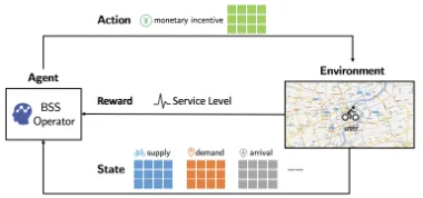
In this paper, we propose a deep reinforcement learn-ing framework for incentivizlearn-ing users to rebalance docke-less BSS, as shown in Figure 1. Specifically, we view the problem as interactions between a bike sharing service op-erator and the environment, and formulate the problem as a Markov decision process (MDP). In this MDP, a state consists of supply, demand, arrival, and other related in-formation, and each action corresponds to a set of mone-tary incentives for each region, to incentivize users to walk to nearby locations and use bikes there. The immediate re-ward is the number of satisfied user requests. Our objec-tive is to maximize the long-term service level, i.e., the to-tal number of satisfied requests, which is of highest inter-est for bike sharing service providers (Lin and Yang 2011). Our approach falls under the topic of incentivizing strate-gies in multi-agent systems (Xue et al. 2016; Tang 2017; Cai et al. 2018).
To tackle our problem, we develop a novel deep
reinforce-ment learning algorithm called the hierarchical
reinforce-ment pricing(HRP) algorithm. The HRP algorithm builds upon the Deep Deterministic Policy Gradient (DDPG) algo-rithm (Lillicrap et al. 2015), using the general hierarchical reinforcement learning framework (Dietterich 2000). Our idea is to decompose the Q-value of the entire area of in-terest into multiple sub-Q-values of smaller regions. The de-composition enables an efficient searching for policies, as it addresses the complexity issue due to high-dimensional in-put space and temporal dependencies. In addition, the HRP algorithm also takes spatial dependencies into consideration and contains a localized module, in order to correct the bias in Q-value function estimation, introduced by decomposi-tion and correladecomposi-tions among sub-states and sub-acdecomposi-tions. Do-ing so reduces the input space and decreases the trainDo-ing loss. We also show that the HRP algorithm improves con-vergence and achieves a better performance compared with existing algorithms.
The main contributions of our paper are as follows:
• We propose a novel spatial temporal bike rebalancing
framework, and model the problem as a Markov decision process (MDP) that aims at maximizing the service level.
• We propose thehierarchical reinforcement pricing(HRP)
algorithm that decides how to pay different users at each time, to incentivize them to help rebalance the system.
• We conduct extensive experiments using Mobike’s
dataset. Results show that HRP drastically outperforms
Figure 1: An overview of the deep reinforcement learning framework for rebalancing dockless bikesharing systems.
state-of-the-art methods. We also validate the optimality
of HRP by comparing with our proposedoffline-optimal
algorithm. We further demonstrate HRP’s generalization ability over different areas.
Related Work
Rebalancing Approaches.With the recent development of BSS, researchers have started to study operational issues leveraging big data (Liu et al. 2017; Yang et al. 2016; Chen et al. 2016; Li et al. 2015), among which rebalancing is one of the most important focuses. Rebalancing approaches can be classified into three categories. The first category adopts the truck-based approach which employs multiple trucks. These methods can reposition bikes either in a static (Liu et al. 2016) or dynamic (Ghosh, Trick, and Varakan-tham 2016) way, for docked BSS. The second category fo-cuses on the use of bike-trailers (O’Mahony and Shmoys 2015; Ghosh and Varakantham 2017; Li, Zheng, and Yang 2018). The third category focuses on the user-based rebal-ancing approach (Singla et al. 2015; Chemla et al. 2013; Fricker and Gast 2016).
Reinforcement Learning.Deep Deterministic Policy Gra-dient algorithm (DDPG) (Lillicrap et al. 2015) builds upon the Deterministic Policy Gradient algorithm (Silver et al. 2014), using deep neural networks to approximate the action-value function for improving convergence. However, conventional reinforcement learning methods cannot scale up to problems with high-dimensional input spaces. Hierar-chical reinforcement learning (Dayan and Hinton 1993) de-composes a large problem into several smaller sub-problems learned by sub-agents, which is suitable for large-scale prob-lems. Each sub-agent only focuses on learning sub-Q-values for its sub-MDP. Thus, the sub-agent can neglect part of the state which is irrelevant to its current decision (Andre and Russell 2002; Van Seijen et al. 2017) to enable faster learn-ing.
Problem Definition
In this section, we introduce and formalize the user-based bike rebalancing problem, i.e., by offering users monetary incentives to motivate them to help rebalance the system.
Consider an area spatially divided into n regions, i.e.,
{r1, r2, ..., rn}. We discretize a day into T timeslots with
equal length, denoted byT = {1,2, ..., T}. LetSi(t)
t ∈ T, i.e., the number of available bikes. We also denote
S(t) = (Si(t),∀i)as the vector of supply. The total user
demand and bike arrival of regionriduring the timeslottis
denoted byDi(t)andAi(t)respectively. We similarly
de-noteD(t) = (Di(t),∀i)andA(t) = (Ai(t),∀i)as the vector of demand and the vector of arrival, respectively. Let
dij(t)denote the number of users intending to ride from
re-gionrito regionrjduring the timeslott.
Pricing Algorithm.At each timeslott, for a user who
can-not find an available bike in his current regionri, a pricing
algorithmAsuggests him alternate bikes inri’s
neighbor-ing regions, denoted byN(ri). Meanwhile,Aalso offers the
user a price incentivepij(t)(in the order of user arrivals), to
motivate him to walk to neighboring regionrj ∈N(ri)to
pick up a bikebhj, wherebhj denotes theh-th bike inrj.A
has a total rebalancing budgetB. When the budget is
com-pletely depleted,Acan no longer make further provision.
User Model.For each userukin regionri, if there are
avail-able bikes in the current region, he takes the nearest one.
Otherwise, there is a walking cost if he walks fromri to a
neighboring regionrj to pick up bikes. We denote the cost
byck(i, j, x), wherexis the walking distance from his loca-tion to the bike. We assume that it has the following form:
ck(i, j, x) =
⎧
⎨
⎩
0 iequals toj
αx2 r
jis a neighboring region ofri
+∞ else
. (1)
This particular form ofck(i, j, x)is motivated by a survey
conducted in (Singla et al. 2015), where it is shown that user cost has a convex structure. Note that this cost is private to each user and the cost function is unknown to the service provider. For a user who cannot find an available bike in
his current regionri, if he receives an offer(pij(t), bhj)and
accepts it, he obtains a utilitypij(t)−ck(i, j, x). Thus, a user
will choose and pick up the bikebhjwhere he can obtain the
maximum utility, and collect the price incentivepij(t). If no
offer leads to a nonnegative utility, the user will not accept any of them, resulting in an unsatisfied request.
Bike Dynamics.Letxijl(t)denote the number of users inri
riding torlby taking a bike inrjat timeslott. The dynamics
of supply in each regionrican be expressed as:
Si(t+ 1) =Si(t)− n
∑
j=1
n
∑
l=1
xjil(t) + n
∑
m=1
n
∑
j=1
xmji(t). (2)
The second and third terms in Eq. (2) denote the numbers of
departing and arriving bikes in regionri. Note that there is a
travel time for bikes travel among regions.
Objective.Our goal is to develop an optimal pricing
algo-rithmAto incentivize users in congested regions to pick up
bikes in neighboring regions, so as to maximize the service level, i.e., the total number of satisfied requests, subject to
the rebalancing budgetB.
Hierarchical Reinforcement Pricing Algorithm
In this section, we present our hierarchical reinforcement
pricing(HRP) algorithm that incentivizes users to rebalance the system efficiently.
MDP Formulation
Our problem is an online learning problem, where an agent interacts with the environment. Therefore, it can be mod-eled as a Markov decision process (MDP) defined by a
5-tuple (S, A, P r, R, γ), where S and A denote the set of
states and actions, P r the transition matrix, R the
imme-diate reward and γ the discount factor. In our problem, at
each timestep t, the state st = (S(t),D(t−1),A(t−
1),E(t−1), RB(t),U(t)). Here,S(t)is the current supply
for each region whileRB(t)is the current remaining budget.
D(t−1),A(t−1)andE(t−1)are the demand, arrival and
the expense in the last timestep for each region.U(t)
repre-sents the un-service rate for each region for a fixed number of past timesteps. The bike sharing service operator takes an action at = (p1t, ..., pnt), and receives animmediate
rewardR(st, at)which is the number of satisfied requests
in the whole area R at timestep t. Specifically,pit
repre-sents the price for regionriat timestept.1 P r(st+1|st, at)
represents thetransition probabilityfrom statestto state
st+1 under actionat. Thepolicy functionπθ(st)with the
parameter θ, maps the current state to a deterministic
ac-tion. The overallobjective is to find an optimal policy to
maximize theoverall discounted rewardsfrom states0
fol-lowingπθ, denoted byJπθ =E[
∑∞
k=0γ
kR(a
k, sk)|πθ, s0],
whereγ ∈ [0,1]denotes thediscount factor. The Q-value
of state st and action at under policy πθ is denoted by
Qπθ(s
t, at) =E[∑∞k=tγ k−tR(s
k, ak)|πθ, st, at].Note that
Jπθis a discounted version of the targeting service level
ob-jective, and will serve as a close approximation whenγ is
close to1. Indeed, our experimental results show that with
γ = 0.99, our algorithm performs very close to the offline
optimal of the service level objective, demonstrating the ef-fectiveness of this approach.
The HRP Algorithm
One of the key challenges in our problem, is that it has a con-tinuous and high-dimensional action space that increases ex-ponentially with the number of regions and suffers from the “curse of dimensionality”. To tackle this problem, we pro-pose the HRP algorithm, which is shown in Algorithm 1. Inspired by hierarchical reinforcement learning and DDPG, the HRP algorithm, which captures both temporal and spa-tial dependencies, is able to address the convergence issue of existing algorithms and improve performance.
Specifically, we decompose the Q-value of the whole area into the sub-value of each region. Then, the Q-value can be estimated by the additive combination of
es-timators of sub-Q-values according to∑n
j=1Qjµj(sjt, pjt),
wheresjt, pjtdenote the sub-state and sub-action of region
rj at timestep t, and µj corresponds to the parameter of
the estimator. For each timestep, the current state depends on previous states as people pick up and return bikes dy-namically. To capture the sequential relationships exhibit in states, one idea is to train each sub-agent using Long
1
To reduce the complexity of the MDP, we employ the policy that the monetary incentives a user in regionrireceives for picking
up bikes in neighboring regions are the same. Thus, we usepitin
Algorithm 1The Hierarchical Reinforcement Pricing (HRP) algorithm.
Require: Randomly initialize weightsθ, µfor the actor networkπθ(s)and the critic networkQµ(s, a).
Initialize target actor networkπ′and target critic networkQ′with weightsθ′←θ, µ′ ←µ
Initialize experience replay bufferBby filling with samples collected from the warm-up phase
forepisode= 1, ..., M do
Initialize a random processN to explore the action space, e.g. Gaussian noise, and receive initial states1
forstept= 1, ..., T do
◃Explore and sample
Select and execute actionat=πθ(st) +Nt(Ntsampled fromN), observe rewardRtand next statest+1
Store transition(st, at, Rt, st+1)in experience replay bufferB//update experience replay bufferB
Sample a random minibatch ofNtransitions(si, ai, Ri, si+1)fromB
◃Get current state-action pair’s Q-value
Compute the decomposed Q-valuesQj
µj(sji, pji)for each regionrj
Compute the bias-correction termfj(sji, N S(si, rj), pji)for each regionrjby the localized module
Compute current state-action pair’s Q-valueQµ(si, ai)according to Eq. (3)
◃Get next state-action pair’s Q-value
Get action for next state by actor network:a′
i+1=πθ′′(si+1)
Compute the decomposed Q-valuesQjµ′
j(sj(i+1), p
′
j(i+1))for each regionrj
Compute the bias-correction termfj(sj(i+1), N S(si+1, rj), p′j(i+1))for each regionrjby the localized module
Compute next state-action pair’s Q-valueQ′
µ′(si+1, a′i+1)according to Eq. (3)
◃Update
Setyi=Ri+γQ′µ′(si+1, a′i+1)
Update the critic by minimizing the loss according to Eq. (5)
Update the actor using the sampled policy gradient according to Eq. (4)
Update the target networks:θ′←τ θ+ (1−τ)θ′, µ′ ←τ µ+ (1−τ)µ′
end for end for
Short-Term Memory (LSTM) (Hochreiter and Schmidhuber 1997) unit, which can capture complex sequential dependen-cies. However, LSTM maintains a complex architecture and needs to train a substantial number of parameters. Note that a key challenge in hierarchical reinforcement learning is to estimate accurate sub Q-values, which leads to an accurate overall Q-value estimation. Thus, we adopt the Gated Recur-rent Unit (GRU) model (Cho et al. 2014), a simplified vari-ant of LSTM. Such a structure is more condensed and has fewer parameters, which enables a higher sample efficiency and avoids overfitting.
However, applying a direct decomposition can lead to a large bias due to the dependence of each region and its neighbors. In our case, users may pick up bikes in neighbor-ing regions besides their current regions, resultneighbor-ing in the fact that actions in different regions are coupled. Therefore, we need to take this domain spatial feature into consideration.
We tackle the bias of Qµ(st, at)and ∑
n j=1Q
j
µj(sjt, pjt)
by embedding the localized module to incorporate the
spa-tial information. For each regionrj, the localized module
(represented byfj) takes not only the statesjt and action
pjt, but also the states of its neighboring regions denoted by
N S(st, rj)as inputs. In particular,fjis approximated by a
neural network consisting of two fully-connected layers for
bias correction. Thus, we estimateQµ(st, at)by:
n
∑
j=1
Qj
µj(sjt, pjt) +fj(sjt, N S(st, rj), pjt). (3)
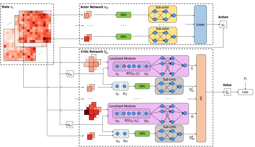
The network architecture we propose to accelerate the search process in a large state space and a large action space is shown in Figure 2. Formally speaking, the key compo-nents of the HRP algorithm are described below:
The Actor:The actor network represents the policyπθ
pa-rameterized byθ. It maximizesJπθusing stochastic gradient
ascent. In particular, the gradient ofJπθoverθis given by:
∇θJπθ =Es∼ρπθ[∇θπθ(s)∇aQµ(s, a)|a=πθ(s)], (4)
whereρπθ denotes the distribution of states.
The Critic:The critic network takes the statestand action
at as input, and outputs the action value. Specifically, the
critic approximates the action-value functionQπθ(s, a)by
minimizing the following loss (Lillicrap et al. 2015):
L(Qπθ) =
Est∼ρπ,at∼π[(Qµ(st, at)−yt)
2
], (5)
whereyt=R(st, at) +γQ
′
µ′(st+1, π
′
θ′(st+1)).
Experiments
Dataset
We make use of a Mobike dataset consisting of users’
tra-jectories from August1st to September 1st in2016, in the
city of Shanghai. Each data record contains the following information: order ID, bike ID, user ID, start time, start lo-cation (specified by longitude and latitude), end time, end
location, and trace, with a total number of102,361orders.
Figure 2: The actor-critic framework of the HRP algorithm.
(a) Demand in 8 a.m.-9 a.m. (b) Demand in 6 p.m.-7 p.m.
Figure 3: The temporal and spatial imbalance problem.
where different colors of circles represent different demand levels with the radius representing the number of demand. As shown, there exists a significant temporal and spatial im-balance.
Experimental Setup
According to Mobike’s trajectory dataset, we obtain spatial and temporal information of users’ requests and arrivals. We observe that the demand curve of different weekdays follows a very similar pattern according to the dataset, where the dis-tribution during a day is bimodal with peaks corresponding to morning and evening rush hours. Thus, we aggregate all weekday demands to recover the total demand of a day. Each
day consists of24timeslots, and each timeslot is1hour. We
serve user requests every minute, where user requests are directly drawn from data while their starting locations (lon-gitude and latitude) follow uniform distribution in their
start-ing regions. To determine the initial distribution of bikes at the beginning of the day, we follow a common and practi-cal way that most bike sharing operators (e.g. Mobike, Ofo) employ to redistribute bikes. The number of initial bikes in
regionriis set as the product of the total supply and the ratio
of the total demand inriand the total demand for the whole
area. Then, locations of initial bikes of each region are ran-domly drawn from data (from the locations of bikes in the corresponding region). Users respond to the system
accord-ing to the defined user model, where the parameterαof the
cost function as in Eq. (1) is selected so that the cost ranges in[0RM B,5RM B]. This is chosen according to a survey conducted by (Singla et al. 2015), which shows that the cost
ranges from0to2euros, and we converted it by the
purchas-ing power of users. Accordpurchas-ing to Mobike, the total number
of orders in China is about20 million, with the total
sup-ply, i.e., number of bikes, in China to be3.65million. Since
we cannot obtain the total supply directly from data, we set
the total supply asO× 3.65
20 (Ois the number of orders in
our system). As the initial supply affects the inherent imbal-ance degree in Mobike’s system, we vary this number in our experiments to evaluate this effect. We use the first-order ap-proximation to compute the number of the unobserved lost demand (O’Mahony and Shmoys 2015).
Configurations of the HRP Algorithm For the state rep-resentation, we choose the fixed number of past timesteps of
U(t)to be8. The comparison is fair as hyperparamters are
the same for comparing reinforcement learning algorithms, following the configuration of (Lillicrap et al. 2015). We
train the algorithm for100episodes in each setting, where
each episode consists of24N steps (N denotes the number
Evaluation Metric
We propose a metric called decreased un-service ratiofor
performance evaluation. This choice can better character-ize the improvement of the pricing algorithm over the orig-inal system (without monetary incentives) in the un-served events, compared with the service level (Singla et al. 2015).
Definition 1. (Decreased un-service ratio)The decreased
un-service number of an algorithmAis the difference
be-tween the number of un-service events (U N) under
Mo-bike and that of A, i.e., DU N(A) = U N(Mobike) −
U N(A).2 The decreased un-service ratio ofAis defined
asDU R(A) = U NDU N(Mobike(A))×100%.
Baselines
We compare HRP with the following baseline algorithms:
• Randomized pricing algorithm (Random): assigns
mone-tary incentives randomly under the budget constraint.
• OPT-FIX (Goldberg, Hartline, and Wright 2001): an
of-fline algorithm to maximize the acceptance rate with full a-priori user cost information.
• DBP-UCB (Singla et al. 2015): a state-of-the-art method
for user-based rebalancing which applied a multi-armed bandit framework.
• DDPG (Lillicrap et al. 2015)
• HRA (Van Seijen et al. 2017): a reinforcement learning
al-gorithm which directly employed reward decomposition.
• Offline-optimal: a pricing algorithm which maximizes the
service level under the budget constraint with known user costs in advance, serving as an upper bound for any on-line pricing algorithms. To reduce the complexity of the formulation, we assume a trip finishes in the same
times-lot (1 hour) it begins.3In our comparison with the
offline-optimal, due to computational complexity, we assume that the costs of users walking from one region to another are
the same for each timeslott, defined asck(i, j, x) =cij(t)
if rj is the neighboring region of ri, where cij(t) is
drawn independently from the empirical distribution of
user costs for picking up bikes inrjinstead of their
cur-rent regionsri defined as Eq. (1) from timeslott of the
dataset. Then, the problem can be formulated as the
fol-2
Note thatU N(Mobike)is computed by simulating Mobike’s original system.
3
Otherwise, one has to set the timeslot as 1 minute, resulting in an integer linear program with too large complexity. Please note that the model and simulation do not rely on the assumption.
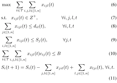
lowing integer linear program:4
max ∑
t∈T
∑
i,j,l∈[1,n]
xijl(t) (6)
s.t. xijl(t)∈Z+, ∀i, j, l, t (7)
∑
j∈[1,n]
xijl(t)≤dil(t), ∀i, l, t (8)
∑
i,l∈[1,n]
xijl(t)≤Sj(t), ∀j, t (9)
∑
t∈T
∑
i,j,l∈[1,n]
xijl(t)cij(t)≤B (10)
Si(t+ 1) =Si(t)−
∑
j,l∈[1,n]
xjil(t) +
∑
l,j∈[1,n]
xlji(t),∀i, t.
(11)
Constraints (8) guarantee that for any timeslot, the
num-ber of users inriheading forrlis no larger than the
de-mand fromritorl. Constraints (9) mean that the number
of bikes picked up inrj does not exceed the bike supply
in this region. Constraint (10) ensures that the money the
service provider spends is limited byB. Constraints (11)
are for the dynamics of the supply of bikes.
Performance Comparison
We first compare HRP and reinforcement learning baselines to analyze the converging issue. Next, we compare HRP with varying budget and supply to evaluate its effectiveness in a day. Then, we analyze the long-term performance.
Fi-nally, we compare HRP with theoffline-optimalscheme and
evaluate its generalization ability.
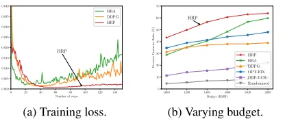
Training Loss Figure 4(a) shows the training loss under HRP, HRA, and DDPG. As expected, DDPG diverges due to high-dimensional input spaces. Notably, HRA diverges with an even larger training loss. This is due to the imprac-tical assumption of independence among sub-MDPs, which results in a biased estimator for the Q-value function. HRP
outperforms the two and is able to converge.5
Effect of Varying Budget Constraints Figure 4(b) shows the decreased un-service ratio of each algorithm under ferent budget constraints. DDPG performs similarly at dif-ferent budget levels as it fails to learn to efficiently use the budget in such a large input space. HRA performs better than DDPG due to the decomposition. HRP decreases the
un-service ratio by43%−63%, and outperforms other
al-gorithms under all budget levels. The reason that OPT-FIX and DBP-UCB underperform HRP is that they do not con-sider spatial information, and focus solely on optimizing the acceptance rate.
Achieving Better Bike Distribution To also analyze the rebalancing effect over a day, we measure how the distribu-tion of bikes at the end of the day diverges from its value at the beginning of the day, using the Kullback-Leibler (KL)
4
We solve the program with Gurobi.
5
0 20 40 60 80 100 120 140 Number of steps 0.000
0.005 0.010 0.015 0.020 0.025 0.030 0.035 0.040
Loss
HRP
HRA DDPG HRP
(a) Training loss.
1000 1200 1400 1600 1800 2000 Budget (RMB) 0 10 20 30 40 50 60 70 Decrease Unservice Ratio (%) HRP HRP HRA DDPG OPT-FIX DBP-UCB Randomized
(b) Varying budget.
Figure 4: Comparison of training loss and varying budget.
HRP HRA DBP-UCB DDPG OPT-FIX
0.548 0.560 0.562 0.586 0.598
Table 1: KL divergence of user-based algorithms.
divergence measure (Kullback and Leibler 1951). We sim-ulate Mobike’s original system (without monetary
incen-tives), and obtain its KL divergence level to be 0.554. As
seen in Table 1, OPT-FIX obtains a bike distribution that is most different from the initial bike distribution. The rea-son can be that OPT-FIX is too aggressive in maximizing the acceptance rate, which can worsen the bike distribution. HRP outperforms all existing algorithms with a KL
diver-gence value of 0.548, even smaller than Mobike’s value.
This demonstrates that HRP is able to improve the bike dis-tribution at the end of a day.
Effect of Varying Supply Besides varying the budget, it is also worth studying how HRP performs under different sup-ply levels to evaluate its robustness. The results are shown in Figure 5(a). Intuitively, the problem is more challenging when supply is limited, which can lead to a large un-service rate. Random and DBP-UCB both perform poorly while the performance of OPT-FIX, DDPG, and HRA are almost the same. HRP performs significantly better than others, and
achieves a 47%−60% decrement in the un-service ratio,
demonstrating its robustness against different total supply.
Long-Term Performance Apart from analyzing one day’s effect, we also evaluate the long-term performance by varying the number of days. We compare HRP with two
most competitive algorithms, HRA and OPT-FIX, from 1
day to5days using decreased un-service number. As shown
in Figure 5(b), HRP outperforms other algorithms. The per-formance gap also gets larger as the number of days in-creases. This is because HRP can achieve a better bike dis-tribution as discussed in the previous section, and it learns to maximize the long-term reward. Readers please refer to the supplemental material for our detailed analysis of the result.
Optimality We now provide comparison results with the
offline-optimalscheme. To avoid computation and memory overhead, we conduct the comparison on a smaller area
con-sisting of3×3regions with highest request density to
eval-uate how well HRP can perform in a most congesting area.
We compare both HRP and HRA with theoffline-optimal,
by adjusting different values of timeslotsV. TheV-timeslot
7000 7500 8000 8500 9000 Total supply (#bikes) 10 20 30 40 50 60 Decrease Unservice Ratio (%) HRP HRP HRA DDPG OPT-FIX DBP-UCB Randomized
(a) Varying supply.
1 2 3 4 5 Number of days 0 2000 4000 6000 8000 10000 12000 14000 16000 Decrease Unservice Num b er HRP HRP HRA OPT-FIX (b) Long-term.
Figure 5: Comparison of varying supply and number of days.
0 8 16 24 Number of Timeslots 25 30 35 40 45 Decrease Unservice Ratio(%) HRA: 40.3% HRP: 44.8% Offline-optimal HRP HRA (a) Optimality.
0 20 40 60 80 100 Decreased Unservice Ratio (%) 0.0
0.2 0.4 0.6 0.8 1.0
CDF
HRP
HRP HRA
(b) Generalization.
Figure 6: Optimality and generalization comparison.
optimization means that for everyV timeslots, we optimize
the offline program withV horizons. Intuitively, a largerV
leads to better performance. In this evaluation, the results
are averaged over400independent runs of each algorithm.
Figure 6a demonstrates that the performance of HRP is very close to that of 24-timeslot optimization, while HRA only performs close to 4-timeslot optimization.
Generalization Now, we investigate whether HRP can transfer well, i.e., trained with certain areas but still performs well when applied to new ones. As the dataset only consists of trajectories in Shanghai, we divide the whole area into
smaller areas where each consists of3×3 regions to
gen-erate more areas. We train HRP and HRA in a certain area and then test them on other areas. Figure 6b shows the cu-mulative density function (CDF) of HRP and HRA on the decreased un-service ratio over all areas. HRP can achieve
a40% −80% un-service ratio decrement over80% areas
in testing. This demonstrates that HRP generalizes well to new areas that it has never seen before. Note that the curve of HRP is strictly to the right of HRA, showing that HRP generalizes better than HRA.
Conclusion
We propose a deep reinforcement learning framework for incentivizing users to rebalance dockless bike sharing sys-tems. We propose a novel deep reinforcement learning
algo-rithm calledhierarchical reinforcement pricing(HRP). HRP
Chinese dockless bike sharing company. Results show that HRP outperforms state-of-the-art methods.
As for future work, one interesting extension is to deploy our algorithm in a real-world bike sharing system. To adapt to shifting environments across the year, one can first update the simulator with latest collected data, and then train HRP with the updated simulator offline every a fixed number of days. After training, one can adopt the new policy online. It is also promising to consider more factors in the user feed-back model, e.g. travel distance and the time of day.
References
Andre, D., and Russell, S. J. 2002. State abstraction for
pro-grammable reinforcement learning agents. InAAAI/IAAI, 119–
125.
Cai, Q.; Filos-Ratsikas, A.; Tang, P.; and Zhang, Y. 2018. Rinforcement mechanism design for fraudulent behaviour in
e-commerce. InProceedings of the 32nd AAAI Conference on
Artificial Intelligence.
Chemla, D.; Meunier, F.; Pradeau, T.; Calvo, R. W.; and Yahiaoui, H. 2013. Self-service bike sharing systems: simu-lation, repositioning, pricing.
Chen, L.; Zhang, D.; Wang, L.; Yang, D.; Ma, X.; Li, S.; Wu, Z.; Pan, G.; Nguyen, T.-M.-T.; and Jakubowicz, J. 2016. Dynamic cluster-based over-demand prediction in bike sharing systems. InProceedings of the 2016 ACM International Joint Confer-ence on Pervasive and Ubiquitous Computing, 841–852. ACM. Cho, K.; Van Merri¨enboer, B.; Gulcehre, C.; Bahdanau, D.; Bougares, F.; Schwenk, H.; and Bengio, Y. 2014. Learning phrase representations using rnn encoder-decoder for statistical
machine translation. InProceedings of the 2014 Conference on
Empirical Methods in Natural Language Processing (EMNLP), 1724–1734.
Dayan, P., and Hinton, G. E. 1993. Feudal reinforcement
learn-ing. In Advances in neural information processing systems,
271–278.
Dietterich, T. G. 2000. Hierarchical reinforcement learning
with the maxq value function decomposition.Journal of
Artifi-cial Intelligence Research13:227–303.
Fricker, C., and Gast, N. 2016. Incentives and redistribution in homogeneous bike-sharing systems with stations of finite
ca-pacity. Euro journal on transportation and logistics5(3):261–
291.
Ghosh, S., and Varakantham, P. 2017. Incentivizing the use of bike trailers for dynamic repositioning in bike sharing systems. Ghosh, S.; Trick, M.; and Varakantham, P. 2016. Robust repo-sitioning to counter unpredictable demand in bike sharing
sys-tems. InProceedings of the Twenty-Fifth International Joint
Conference on Artificial Intelligence, IJCAI’16, 3096–3102. AAAI Press.
Goldberg, A. V.; Hartline, J. D.; and Wright, A. 2001.
Compet-itive auctions and digital goods. InProceedings of the twelfth
annual ACM-SIAM symposium on Discrete algorithms, 735– 744. Society for Industrial and Applied Mathematics.
Hochreiter, S., and Schmidhuber, J. 1997. Long short-term
memory.Neural computation9(8):1735–1780.
Kullback, S., and Leibler, R. A. 1951. On information and
sufficiency.The annals of mathematical statistics22(1):79–86.
Li, Y.; Zheng, Y.; Zhang, H.; and Chen, L. 2015. Traffic
pre-diction in a bike-sharing system. InProceedings of the 23rd
SIGSPATIAL International Conference on Advances in Geo-graphic Information Systems, 33. ACM.
Li, Y.; Zheng, Y.; and Yang, Q. 2018. Dynamic bike repo-sition: A spatio-temporal reinforcement learning approach. In
Proceedings of the 24th ACM SIGKDD International Confer-ence on Knowledge Discovery and Data Mining, 1724–1733. ACM.
Lillicrap, T. P.; Hunt, J. J.; Pritzel, A.; Heess, N.; Erez, T.; Tassa, Y.; Silver, D.; and Wierstra, D. 2015. Continuous control with
deep reinforcement learning.arXiv preprint arXiv:1509.02971.
Lin, J.-R., and Yang, T.-H. 2011. Strategic design of public
bicycle sharing systems with service level constraints.
Trans-portation research part E: logistics and transTrans-portation review
47(2):284–294.
Liu, J.; Sun, L.; Chen, W.; and Xiong, H. 2016. Rebalancing bike sharing systems: A multi-source data smart optimization. InProceedings of the 22nd ACM SIGKDD International Con-ference on Knowledge Discovery and Data Mining, 1005–1014. ACM.
Liu, J.; Sun, L.; Li, Q.; Ming, J.; Liu, Y.; and Xiong, H. 2017. Functional zone based hierarchical demand prediction for bike
system expansion. InProceedings of the 23rd ACM SIGKDD
International Conference on Knowledge Discovery and Data Mining, 957–966. ACM.
O’Mahony, E., and Shmoys, D. B. 2015. Data analysis and
optimization for (citi) bike sharing. InAAAI, 687–694.
Shaheen, S.; Guzman, S.; and Zhang, H. 2010. Bikesharing in
europe, the americas, and asia: past, present, and future.
Trans-portation Research Record: Journal of the TransTrans-portation Re-search Board(2143):159–167.
Silver, D.; Lever, G.; Heess, N.; Degris, T.; Wierstra, D.; and Riedmiller, M. 2014. Deterministic policy gradient algorithms. In Proceedings of the 31st International Conference on Ma-chine Learning (ICML-14), 387–395.
Singla, A.; Santoni, M.; Bart´ok, G.; Mukerji, P.; Meenen, M.; and Krause, A. 2015. Incentivizing users for balancing bike
sharing systems. InAAAI, 723–729.
Tang, P. 2017. Reinforcement mechanism design. In
Pro-ceedings of the Twenty-Sixth International Joint Conference on Artificial Intelligence, IJCAI-17, 5146–5150.
Van Seijen, H.; Fatemi, M.; Romoff, J.; Laroche, R.; Barnes, T.; and Tsang, J. 2017. Hybrid reward architecture for
reinforce-ment learning. InAdvances in Neural Information Processing
Systems, 5392–5402.
Xue, Y.; Davies, I.; Fink, D.; Wood, C.; and Gomes, C. P. 2016. Avicaching: A two stage game for bias reduction in citizen
sci-ence. InProceedings of the 2016 International Conference on
Autonomous Agents & Multiagent Systems, 776–785. Interna-tional Foundation for Autonomous Agents and Multiagent Sys-tems.
Yang, Z.; Hu, J.; Shu, Y.; Cheng, P.; Chen, J.; and Moscibroda, T. 2016. Mobility modeling and prediction in bike-sharing
sys-tems. InProceedings of the 14th Annual International