AN EDGE BASED ALGORITHM FOR FRACTAL IMAGE COMPRESSION

208 |

P a g e

AN EDGE BASED ALGORITHM FOR FRACTAL

IMAGE COMPRESSION

1

Shipra Gupta,

Shipra,

Neha Sahu,

Gagan Minocha,

Paurush Bhulania

12345

Amity School of Engineering And Technology, Noida (India)

ABSTRACT

With the continuous growth of modern technology, demand for image transmission and storage is increasing

rapidly. Advance in computer technology for mass storage and digital processing paved way for implementing

advanced data compression techniques .Fractal image is a new technique for encoding images compactly. It is

based on local self similarity within images. This compression technique gives higher compression ratio with

moderate image quality. In this algorithm instead of searching entire domain image it will search in the edges.

This compression technique is superior to the other existing methods and compression ratio as high as 100 is

possible. In the decoding technique the quality of image becomes better with each iteration.

Key words

:

Fractal, iterative, encoding, contrast, brightness

1. INTRODUCTION

Data compression is the process of transforming the data description into a more succinct and condensed

form [3]. This improves storage efficiency, communication speed, and security. These facts justify the efforts, of

private companies and universities, on new image compression algorithms. Images are stored on computers as

collections of bits (a bit is a binary unit of information which can answer “yes” or “no” questions) representing

pixels or points forming the picture elements [2]. Since the human eye can process large amounts of

information (some 8 million bits), many pixels are required to store moderate quality images.

Most data contains some amount of redundancy, which can sometimes be removed for storage and

replaced for recovery, but this redundancy does not lead to high compression ratios. An image can be

changed in many ways that are either not detectable by the human eye or do not contribute to the

degradation of the image [1]. So how can image data be compressed? Fortunately, the human eye is not

sensitive a wide variety of information loss [2].That is, the image can be changed in many ways that are

either not detectable by the human eye or do not contribute to degradation of the image. If these changes are

made so that the data becomes highly redundant, then the data can be compressed when the redundancy can be

detected. Fractal image compression is a lossy technique proposed by Michael Barnsley and Alan Sloan in

1988, based on their work at the Georgia Institute of Technology [4]. Barnsley was the first to propose the

notion of Fractal Image Compression by which real life objects would be modeled by deterministic fractal

objects. The fractals that one can easily generate with an iterated function system are all of a particular type. It

was Michael Barnsley and his research group from the Georgia Institute of Technology who first saw and

realized the potential of iterated function systems for modeling of, e.g., clouds, trees, and leaves [3]. Fractal

209 |

P a g e

techniques are introduced in computer science for natural phenomena. The new idea comes from natural theory

called iterated function system.(IFS). Michael Barnsley and his research group from Georgia Institute of first

saw and realized the potential of iterated function systems for modeling of clouds, trees etc. The fractals that

can generate with iterated function systems are of particular type . Thus in an IFS coding of a picture of face one

should observe tiny distorted copies of face everywhere. This seemed not only unnatural but also technically

infeasible. In 1989 ,Arnaud Jacquin one of the graduate students of Barnsley ,realized the first automatic

fractal encoding systems in his dissertation ,leaving behind the rigid thinking in terms of global IFS mappings.

This broke the ice for new direction research in image coding [4][5].

1.1 FRACTAL GOLDRUSH

The basic new ideas in Jacquin‟s approach was simple. An image should not thought be thought of as a collage

copies of entire ,but copies of smaller parts of it. The general approach is to subdivide the image into a partion

into fixed size square blocks and then to find matching image portion of each part.. This set up has been known

as local or partitioned iterated function system(PIFS).

1.2

WHAT IS FRACTAL IMAGE COMPRESSION?

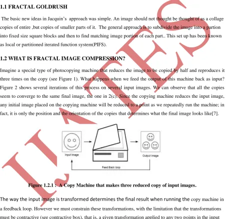
Imagine a special type of photocopying machine that reduces the image to be copied by half and reproduces it

three times on the copy (see Figure 1). What happens when we feed the output of this machine back as input?

Figure 2 shows several iterations of this process on several input images. We can observe that all the copies

seem to converge to the same final image, the one in 2(c). Since the copying machine reduces the input image,

any initial image placed on the copying machine will be reduced to a point as we repeatedly run the machine; in

fact, it is only the position and the orientation of the copiesthat determines what the final image looks like[7].

Figure 1.2.1 : A Copy Machine that makes three reduced copy of input images.

The way the input image is transformed determines the final result when running the

a feedback loop. However we must constrain these transformations, with the limitation that the transformations

must be contractive (see contractive box), that is, a given transformation applied to any two points in the input

image must bring them closer in the copy. This technical condition is quite logical, since if points in the copy

were spread out the final image would have to be of infinite size. Except for this condition the transformation

can have any form. In practice, choosing transformations of the form

210 |

P a g e

is sufficient to generate interesting transformations called affine transformations of the plane. Each can skew,

stretch, rotate, scale and translate an input image. A common feature of these transformations that run in a loop

back mode is that for a given initial image each image is formed from a transformed (and reduced) copies of

itself, and hence it must have detail at every scale. That is, the images are fractals[6][9].

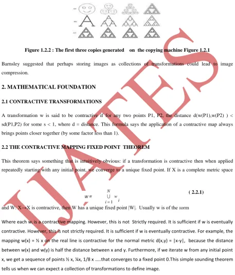
Figure 1.2.2 : The first three copies generated on the copying machine Figure 1.2.1

Barnsley suggested that perhaps storing images as collections of transformations could lead to image

compression.

2. MATHEMATICAL FOUNDATION

2.1 CONTRACTIVE TRANSFORMATIONS

A transformation w is said to be contractive if for any two points P1, P2, the distance d(w(P1),w(P2) ) <

sd(P1,P2) for some s < 1, where d = distance. This formula says the application of a contractive map always

brings points closer together (by some factor less than 1).

2.2 THE CONTRACTIVE MAPPING FIXED POINT THEOREM

This theorem says something that is intuitively obvious: if a transformation is contractive then when applied

repeatedly starting with any initial point, we converge to a unique fixed point. If X is a complete metric space

and W: X→X is contractive, then W has a unique fixed point |W|. Usually w is of the form

Where each wi is a contractive mapping. However, this is not Strictly required. It is sufficient if w is eventually

contractive. However, this is not strictly required. It is sufficient if w is eventually contractive. For example, the

mapping w(x) = ½ x on the real line is contractive for the normal metric d(x,y) = |x-y|, because the distance

between w(x) and w(y) is half the distance between x and y. Furthermore, if we iterate w from any initial point

x, we get a sequence of points ½ x, ¼x, 1/8 x …..that converges to a fixed point 0.This simple sounding theorem

tells us when we can expect a collection of transformations to define image.

2.3 COLLAGE THEOREM:

Let (Y, dY ) be a complete metric space. Given an

 N

i i

w

1

 W

=

211 |

P a g e

suppose that there exists a contractive map f on Y with contractivity factor 0 ≤ c < 1 such that

If is the fixed point of

then

So if one wishes to approximate a function y with the fixed point of an unknown contractive map f, it is only

needed to solve the inverse problem of finding f which minimizes the collage distance dY (y,f(y)). The main result in Forte and Vrscay that we will use to build one of the IFSs estimators is that the inverse problem can be reduced to minimize a suitable quadratic form in terms of the pi given a set of affine maps wi and the sequence

of moments gk of the target measure.Let

be the simplex of probabilities. Let w = (w1,w2, . . . ,wn), N = 1, 2, . . . be subsets of W = {w1,w2, . . .} the

infinite set of affine contractive maps on X = [0, 1] and let g the set of the moments of any order of

Denote by M the Markov operator of the N-maps IFS (w, p) and by[4]

, with associated moment vector of any order hN. The collage distance between the moment vector of

is a continuous function and attains an absolute minimum value Δ min on ΠN

3. ITERATED FUNCTION SYSTEMS

Before we proceed with the image compression scheme, we will discuss the copy machine example with some

notation. Running the special copy machine in a feedback loop is a metaphor for a mathematical model called an

iterated function system (IFS). An iterated function system consists of a collection of contractive

transformations; discuss the copy machine example with some notation. Running the special copy machine in a

feedback loop is a metaphor for a mathematical model called an iterated function system (IFS). An iterated

function system consists of a collection of contractive transformations.{ wi : R2 | i = 1…n } which map the

plane R2 to itself. This collection of transformations define a map

W (.) = wi(.)

(2.3.1)

(2.3.2)

(2.3.3)

(2.2.1)

(2.3.4)

(2.3.5)

(2.3.7)

212 |

P a g e

The map W is not applied to the plane, it is applied to sets that is, collections of points in the plane. Given

input set S, we can compute wi (S) for each i, take the union of these sets, and get a new set W(S). So W is a map on the space of subsets to the plane. We call these transformations „Block wise‟ transformations. An

important fact proved by Hutchinson is that when the wi are contractive in the plane, then W is contractive in a

space of (closed and bounded) subsets of the plane. Hutchinson‟s theorem allows us to use the contractive

mapping fixed point theorem (see box), which tells us that the map W will have a unique fixed point in the

space of all images. That is, whatever image (or set) we start with, we can repeatedly apply W to it and we will

converge to a fixed image. Thus W (or the wi ) completely describe a unique image. In other words, given an

input image f0, we can run the copying machine once to get f1 = W(f0), twice to get f2 = W(f1) =W(W(f0)) =

Wo2(f0), and so on. The attractor, which is the result of running the copying machine in a feedback loop, is the

limit set which is not dependent on the choice of f0. Iterated function systems are interesting in their own right,

but we are not concerned with them specifically. We will generalize the idea of the copy machine and use it to

encode gray scale images.

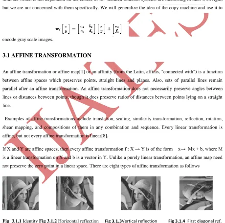
3.1 AFFINE TRANSFORMATION

An affine transformation or affine map[1] or an affinity (from the Latin, affinis, "connected with") is a function

between affine spaces which preserves points, straight lines and planes. Also, sets of parallel lines remain

parallel after an affine transformation. An affine transformation does not necessarily preserve angles between

lines or distances between points, though it does preserve ratios of distances between points lying on a straight

line.

Examples of affine transformations include translation, scaling, similarity transformation, reflection, rotation,

shear mapping, and compositions of them in any combination and sequence. Every linear transformation is

affine, but not every affine transformation is linear[8].

If X and Y are affine spaces, then every affine transformation f : X → Y is of the form x→ Mx + b, where M

is a linear transformation on X and b is a vector in Y. Unlike a purely linear transformation, an affine map need

not preserve the zero point in a linear space. There are eight types of affine transformation as follows

213 |

P a g e

Fig 3.1.5 Fig 3.1.6 Fig 3.1.7 Fig 3.1.8

180° rotation 270° rotation Second diagonal reflection 90° rotation

4. FRACTAL IMAGE CODING

Suppose we are dealing with an image of 256×256 in which each pixel consists of one of 256 gray levels called

Range image. We then average an down sample the image into 128×128 size called domain image. We

partitioned both images into blocks of 8×8 pixels sizes. We performed the following affine transformations

to each block domain image Di,j = si Di,j +oi

Where si - [0,1], si €R and oi € [-255,255] oi €Z. In this case we are trying to find linear transformations of

our domain block to arrive to the best [11][12]approximation of a given Range block. Each domain block is

transformed and of our domain block to arrive to the best approximation of a given Range block. Each domain

block is transformed and then compared to each range block Rk,l [7][8]. The comparison process is done by

sliding a window of size 8×8 on the domain block. . The window is moved to one pixel value right and again

comparison is done with the Range block. For a domain image of 128× 128 size the number of comparison done

will be 121×121 number of times. We will determine the values of si, oi which minimizes the mean square

error. The formula of si, oi is given below[2].

            n i n i i D i D n n i n i n i i R i D i R i D n i s 1 1 ) 2 ( 2 2

1 1 1

) )( ( ) ( 2 2 1 1 n n i n i i D i s i R i o      And

Where m, n , Ns =2 or 4(size of blocks)

The value of Si and Oi should be quantized.The formula used for quantizing the values of Si and Oi is given

by[10].

Here we have taken 4 bits for si and 7 bits for oi to quantize. We can even quantize by taking 5 bits for si and 7

bits for oi. Each transformed domain block is compared to each range block i.e. T(Di,j) is compared to each

range block Rk,l in order to find the closest domain block to each range block. This comparison is performed

using the following distortion measure.

(4.1)

(4.2)

214 |

P a g e

Each distortion is stored and the minimum is chosen. The transformed domain block which is found to be the

best approximation for the current range block is assigned to that range block, i.e. the coordinates of the domain

block along with its a and to are saved into the file describing the transformation. This is what is called the

Fractal Code Book[4].

4.1 ENCODING ALGORITHM

1.Suppose the domain image consists 256×256 blocks, average and down sample the range image

to create the domain image of 128×128 blocks.

2.Partition the range (R) and domain images into 4×4 (or) 8×8 (or) 16×16 blocks.

3.For each block of range image rigorously such

4. For each block of range image rigorously such its approximation block in the domain image within

the edges of the image.

5.We have to use the eight types of isometrics(Rotate 00 ,Rotate 900,Rotate - 900,Rotate

1800,Rotate -1800,Rotate 450,Rotate -450,Rotate 2700)

6. Find the contrast (si) ,brightness (oi) and the RMS error of the image. The domain block will be

the best match of range block which gives lowest RMS error.

7.Store the x,y co-ordinates of the domain block, the contrast(si), brightness(oi) and the types of

isometrics used.

8.This will be the fractal code for the range image.

4.2 DECODING ALGORITHM

1. Take an image of any size and find its domain image by averaging and down sampling the range image.

2. Read the fractal code and fetch the corresponding domain block from corresponding x,y co-ordinate of

the fractal code.

3. Rotate the block with the isometrics used in the fractal code.

4. Multiply the contrast and add the brightness with the corresponding block.

5. Use this method for the entire fractal code to create the new image.

6. Repeat step 1 to 6 for seven times to get the original image.

7.

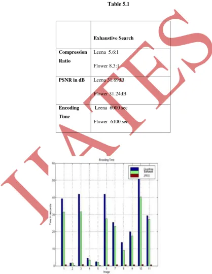
5. RESULTS

215 |

P a g e

Table 5.1

Fig. 5.3 Shows The Bar Graph of Encoding time, of Various Techniques

Exhaustive Search

Compression

Ratio

Leena 5.6:1

Flower 8.3:1

PSNR in dB Leena 31.69dB

Flower 31.24dB

Encoding

Time

Leena 6000 sec

216 |

P a g e

6. CONCLUSION AND FUTURE SCOPE

Using this fractal image compression technique we achieved better image compression ratio and the quality of

image becomes better with each iteration. We have decreased the encoding time to a significant amount. The

encoding time can be further reduced by using parallel processing and genetic algorithm.

REFERENCES

[1] An introduction to fractal image compression ,http//www.s.ti.com/psheets/bpra065.pdf.

[2] Y.Fisher, “Fractal image compression, Siggraph „92‟ course notes”.

[3] Kosmas karadimitrion , “set redundancy , the enhanced compression ,model and methods for compressing images”, PhD Thesis , Lousiana state university,1999.

[4] Venu Gopalpuram, “Image coding based on fractal theory of iterative contractive image

transformations”,1999.

[5] Yuval Fisher, Fractal image compression theory and application, Springer –veralag,1995.

[6] http//www.njcmr.org/ ~mxr0096/thesis.ps.gz.

[7] Dietmar Saupe, Raouf Hamzaaouri, Hannes Hartnstein, “Fractal Image compression an

introductory overview”, ftp://ftp.informatik.Uni-freiburg,DE/documents /paper/fractal.

[8] Arnand E. Jacquin, “ A Novel Fractal block-coding Technique for digital images” ,Geogia Institute of

Technology ,Atlanta, 1989 .

[9] Mathias Ruhl, “Fractal based compression : Adaptive portioning and complexity” , PhD. Thesis

,Albert-Ludwigs - University,1997.

[10] Barnsley.M, “Fractals Everywhere”, San Diego ,1989.