CONTROL OF CONCENTRATION IN
CSTR USING DMC AND
CONVENTIONAL PID BASED ON
RELAY FEEDBACK METHOD
S. SRINIVASULU RAJU Assistant Professor
Dept. of E. Con. E
Sree Vidyanikethan Engineering College [email protected] M. AYEESHA SIDDIQA
III B-Tech Dept. of E. Con. E
Sree Vidyanikethan Engineering College [email protected]
T.K.S. RAVI KIRAN III B-Tech Dept. of E. Con. E
Sree Vidyanikethan Engineering College [email protected]
M. VISWANATH III B-Tech Dept. of E. Con. E
Sree Vidyanikethan Engineering College [email protected] Abstract:
This paper presents the design of a Dynamic Matrix Controller (DMC) is analyzed for concentration control of Continuous Stirred Tank Reactors (CSTRs) which have strong nonlinearities. Various control approaches have been applied on CSTR to control its parameters. All the industrial process applications require solutions of a specific chemical strength of the chemicals or fluids considered for analysis. Such specific concentrations are achieved by mixing a full strength solution with water in the desired proportions. For this, we use two controllers DMC and PID and analyzed. The basic PID controllers have difficulty in dealing with complex nonlinear processes. Simulation studies give satisfactory results. In this paper the control the concentration of one chemical with the help of other has been analyzed. Model design and simulation are done in MATLAB/SIMULINK, using programming. The concentration control is found better controlled with the addition of DMC instead of PID controller solely.
Keywords: CSTR; PID; Relay feedback; Auto-tuning; DMC; MATLAB/SIMULINK. 1. Introduction:
of the most important step
s
is the development of step-response model to describe the system dynamics. First one is when the exact nonlinear theoretical model is given, the step-response model can be found by the linearization of the nonlinear model.2. CSTR Modeling:
Chemical reactions in a reactor are either exothermic or endothermic and therefore require that energy either be removed or added to the reactor for a constant temperature to be maintained. Fig.1 illustrates the schematic of the CSTR process. In the proposed CSTR, an irreversible exothermic reaction takes place. The heat of the
reaction is removed by a coolant medium that flows through a jacket around the reactor. A fluid stream A is fed
to the reactor. A catalyst is placed inside the reactor. The fluid inside the reactor is perfectly mixed and sent out through the exit valve. The jacket surrounding the reactor also has feed and exit streams. The jacket is assumed to be perfectly mixed and at a lower temperature than the reactor [9], [11]. The mathematical model equations are obtained by a component mass balance (1) and energy balance principle (2) in the reactor.
Fig.1: Continuous Stirred Tank Reactor Process
In this paper, CSTR has been considered in which concentration of two chemicals is controlled for better results, the chemical ‘X’ and ‘Y’ and the byproduct is ‘Z’. Ethylene oxide (X) is reacted with water (Y) in a continuously stirred tank reactor (CSTR) to form ethylene glycol (Z). Assume that the CSTR is manipulated at a constant temperature and that the water is in large excess. The stoichoimetric equation is
1
The reactant conversion in a chemical reactor is a function of residence time or its inverse, the space velocity. For an isothermal CSTR, the product concentration can be controlled by manipulating the feed flow rate, which changes the residence time (for a constant volume reactor). It is convenient to working molar units when writing
components balances, particularly if chemical reaction is involved. Let CX and CZ represent the molar
concentration of X and Z (mol/volume).
2
3
Where rx and rz represent rate of generation of species X and Z per unit volume, and Cxi represents the inlet
concentration of species X. If the concentration of the water change than the reaction rate is second order with respect to the concentration of Ethylene oxide
4
Where k1, k2 and k3 are the reaction rate constants and the minus sign indicate that X is consumed in the
reaction. Each mole X reacts with a mole of Y and produces one mole of Z. So the rate of generation of Z is
5
Expanding the left hand side of equation (1)
6
Combining eq (1) and (5)
Similarly,
1 2 8
Z
Z X Z
dC F
C k C k C
dt V
3. Problem formulation:
The linear space model or case study of CSTR is given by
9 10
x Ax Bu
y Cx Du
where the states, inputs and output are in deviation variable form. The first input (dilution rate) is manipulated and the second (feed concentration of A) is a disturbance input. Linearization of two modeling equations (from equations (6) and (7)) at steady state solution to find the following state space matrices is done:
/ 1 2 3 0
1 / 2
/ 0 0 1
0 0
Fs V K K Cxs
A
K Fs V K
Cxfs Cxs Fs V
B Czs C D
For the particular reaction under consideration, the rate constants are k1=5/6/min k2=5/3/min k3=1/6
mol/liter.min. Based on the steady state operating point of CXs=3 gmol/liter, CZs= 1.117gmol/liter and
Fs/V=0.5714 min-1. The state model is
2.4048 0 0.83333 2.2381 7 0.5714 1.117 0 0 1 0 0 A B C D The manipulated input output process transfer function is calculated with the help of
MATLAB.
2
1.117 3.1472 11 4.6429 5.3821 p s G s s s
4. Control methods:
4.1 PID Controller:
When the characteristics of a plant are not suitable, they can be changed by adding a compensator [3] in the control system. One of the simple and useful compensators feedback control design is described in this section. In this paper, the control method is designed based on the time-dimension performance specifications of the system,
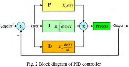
A PID controller calculates an “error” value as the difference between a measured process variable and a desired set point. The controller attempts to minimize the error by adjusting the process control inputs.
Fig. 2 Block diagram of PID controller
Three parameters Kd, KP and KI must be adjusted in the PID controller. In guaranteeing stability and
4.2 Relay Feedback Test:
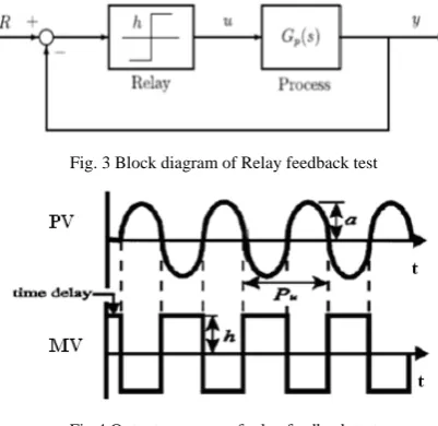
The Astrom and Hagglund relay feedback test is based on the observation that when the output lags behind the
input by radians, the closed-loop system can oscillate with a period of Pu. The block diagram of relay
feedback test is shown in fig.3. The output response of relay feedback test is shown in fig.4. From the response we can find the parameters are ultimate gain and ultimate period Equations (12) and (13).
Fig. 3 Block diagram of Relay feedback test
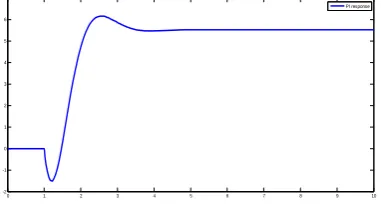
Fig.4 Output response of relay feedback test
A relay of magnitude h is inserted in the feedback loop. Initially, the input u(t) is increased by h. Once the
output y(t) starts increasing after a time delay (D), there lay switches to the opposite direction, u(t)-h. Because
there is a phase lag of– , a limit cycle of amplitude a is generated as shown in fig.4. The period of the limit
cycle is the ultimate period, Pu. The approximate ultimate gain, Ku, and the ultimate frequency, wu are
12
2
13
4.3 Dynamic Matrix Controller:
DMC were developed for cutler and Ramaker [12], and it has been used in the industrial world, mainly in the petrochemical industries. The model response to a unit step change is used to predict the future response of the dependent variables and formulates a series of control action for all the independent variables and formulates a series of control actions for all the independent variables. The actions are selected to minimize the error of the process on the time horizon.
ˆ 14
This is written in the form
15
Where is the prediction at time step k, and is the manipulated input N steps in the past. The
model-predicted output is unlike to be equal to the actual measured output at time step k. The difference between the
measured output ) and the model prediction is called the additive disturbance.
16
The “corrected prediction” is equal to the actual measured output at step k,
ˆ ˆ 17
Similarly, the corrected predicted output at the first time step in the future can be found from
18
19
20
21
∑ ∑ 22
Which we write using matrix-vector notation
23
The corrected-predicted output response is naturally composed of a “forced response” (contributions of the current and future control moves) and a “free response” (the output changes that r predicted if there are no future control moves). The difference between the set point trajectory, r, and the future prediction is
, ,
24
This can be written as
25
Where the future predicted errors are composed of “free response”€ and “forced response” (- )
contributions.
The least-squares objective function (Equ.25) is
26
Notice that the quadratic terms can written in matrix-vector form as
… 27
and
…
… 00
0 0 0 0
0 0
0 0 0
0 28
Therefore the objective function can be written in the form
29
Subject to the modeling equation quality constraint (Equ.25)
30
Substituting (Equ.25) into (Equ.29), the objective function can be written
31
The solution for the minimization of the objective function is
Δu STS w ST E 32
4.4 DMC tuning parameters:
Model Length N: N is an important factor .it affects the step response coefficient as well as the
disturbance response coefficients. It is related to the sampling period T by the relation that T=NΔt
where Δt is the sampling interval.
Prediction horizon length p: p determines how fair into the future the control objective reaches and thus includes the main dynamic characteristics of the target.
stability of the system while larger M results in excessive control action and increases the flexibility, but it may leads to instability.
5. Simulation Results:
Fig .5: Open loop response of concentration of CSTR process.
The response of modeling of concentration of CSTR process is shown in fig 5. From the figure we can observe that a change occur in the coolant of CSTR causes the small change in the concentration of CSTR process.
Fig.6: Response of the CSTR process for Relay feedback test.
The response of the process for relay input is shown in fig 6. From the fig.6 we can observe that the output
exhibits the sustained oscillations. From the above Process response calculated the Ultimate Period (Pu) and
Ultimate gain (Ku). These parameters are used to calculate the controller settings for tracking the change in the
set point.
Fig.7: Servo response of the process for change in set point.
Fig.8: Variation in manipulated input for while tracking the set point.
0 10 20 30 40 50 60 70 80 90 100
8.5695 8.5695 8.5696 8.5696 8.5697 8.5697 8.5698
Concentrtion of CSTR
0 1 2 3 4 5 6 7 8 9 10
-0.4 -0.3 -0.2 -0.1 0 0.1 0.2 0.3 0.4
Response of Process for relay input
0 10 20 30 40 50 60 70 80 90 100
-4 -2 0 2 4 6 8 10 12 14 16
Process Output Set point
0 1 2 3 4 5 6 7 8 9 10
-2 -1 0 1 2 3 4 5 6 7
A step change is made in concentration of CSTR for tracking the set point. The PID tuning parameters are
calculated using the Ziegler and Nichols tuning rules. The servo response for control the concentration of the
CSTR process using conventional PID is shown in Fig 7. From the above graph we conclude that the settling time will be more due to the dominant process lag occurred in the process. Fig.8 shows the variation in the manipulated inputs while tracking set point trajectory.
Fig.9: Servo and regulatory response of CSTR process.
The servo response of concentration control of the CSTR process is done using conventional PID control using Relay feedback test method is shown in fig 9. From the above graph we conclude that the PID controller settings able to track the set point for change in inlet temperature of CSTR and also it can able to satisfy the servo response even in the presence of the disturbance occurred in the process.
Fig.10: The Coefficients of the step response of the CSTR process.
Fig.11: Step response of model of the CSTR process.
DMC control is based on a discrete time step response model that calculates a desired value of the manipulated value that remains unchanged during the next time step. The step response coefficients of the transfer function of the CSTR are shown in fig 10. From the generated step response data we have taken 20 predicted horizon points for formulating the dynamic matrix. Using the dynamic matrix that formed from step response data least square objective function was formulated to find out future control moves for unconstrained DMC.
0 5 10 15
-10 -5 0 5 10 15 20
Set Point Process Output
0 5 10 15 20 25 30 35 40 45 50
-0.1 0 0.1 0.2 0.3 0.4 0.5 0.6
discrete time index, i
s(i
)
step response coefficients
0 0.5 1 1.5 2 2.5 3 3.5 4
-0.1 0 0.1 0.2 0.3 0.4 0.5 0.6
step responses of model and plant
Time (sec)
A
m
pl
itud
Fig.12: The servo response for concentration control of CSTR using DMC.
The DMC settings are Prediction horizon = 20 and the Control horizon = 2 and the model length =50. The response of the DMC controller is shown in Fig 12. This result shows that the concentration of CSTR process is successfully controlled by DMC based on the step-response model obtained by the process test. From the fig.12 we can observe that DMC had lower overshoot and faster response time toward the desired control limits compared to conventional PID controller.
6. Conclusion:
This paper presents an application of Dynamic Matrix Control (DMC) to control the concentration of CSTR process. Firstly, conventional PID controller was implemented by conducting the relay feedback test. From the
response calculated the values of Ku and Pu. From these the PID tuning parameters are calculated using Z-N
closed loop tuning rules to track the change in concentration of the CSTR process. The step-response models are obtained by using the process step test data. The DMC simulation shows satisfactory results with the process. The concentration of CSTR process can be effectively controlled by the DMC. DMC showed faster response time in reaching the desired control limit and actual set point for controlling CSTR process. From the above fig.7 & 12, it can be concluded that DMC performance is better compare to PID in view of tracking the desired set point.
7. Future Work:
The controller for concentration can be implemented by using Quadratic Dynamic Matrix Control to track the servo response and regulatory response. The performance indices will be carried out by using Qualitative and Quantitative comparison of the process. The adaptive Controllers like Model Reference Adaptive Controller, STR, LQR can be implemented for CSTR process for satisfactory desired performance.
8. References:
[1] Aidan O’Dwyer, “Hand book of PI and PID controller tuning rules”,3rd edition page no.78 [2] Bowman, M., Debray, S. K., and Peterson, L. L. 1993. Reasoning about naming systems.
[3] Brown, L. D., Hua, H., and Gao, C. 2003. A widget framework for augmented interaction in SCAPE.
[4] Clarke, D.W. “Application of Generalized Predictive Control to Industrial Processes,” IEEE Cont. Sys. Mag., 49-55, April (1988). [5] Ding, W. and Marchionini, G. 1997 A Study on Video Browsing Strategies. Technical Report. University of Maryland at College Park. [6] Forman, G. 2003. An extensive empirical study of feature selection metrics for text classification. J. Mach. Learn. Res. 3 (Mar. 2003),
1289-1305.
[7] Fröhlich, B. and Plate, J. 2000. The cubic mouse: a new device for three-dimensional input. In Proceedings of the SIGCHI Conference on Human Factors in Computing Systems.
[8] Sannella, M. J. 1994 Constraint Satisfaction and Debugging for Interactive User Interfaces. Doctoral Thesis. UMI Order Number: UMI Order No. GAX95-09398., University of Washington.
[9] Spector, A. Z. 1989. Achieving application requirements. In Distributed Systems, S. Mullender. [10] Tavel, P. 2007 Modeling and Simulation Design. AK Peters Ltd.
[11] V.R.Ravi, T.Thyagarajan, “Application of adaptive control technique to interacting Non Linear Systems”, IEEE 2011 pp 386-392. [12] Y.T. Yu, M.F. Lau, "A comparison of MC/DC, MUMCUT and several other coverage criteria for logical decisions", Journal of
Systems and Software, 2005, in press.
0 1 2 3 4 5 6
-0.5 0 0.5 1
y
time plant output
0 1 2 3 4 5 6
0 2 4 6
u