ADVANCING MOLECULAR DYNAMICS SIMULATIONS OF AQUEOUS IONIC SOLUTIONS
Yi Yao
A dissertation submitted to the faculty at the University of North Carolina at Chapel Hill in partial fulfillment of the requirements for the degree of Doctor of Philosophy in the Department of
Chemistry in the College of Arts and Sciences.
Chapel Hill 2018
Approved by:
Yosuke Kanai
Max L. Berkowitz
Yue Wu
Joanna Atkin
c 2018
Yi Yao
ABSTRACT
Yi Yao: Advancing Molecular Dynamics Simulations of Aqueous Ionic Solutions
(Under the direction of Yosuke Kanai and Max L. Berkowitz)
An understanding of aqueous ionic solutions is essential in developing a mechanistic view of many
biological systems, industrial processes and others. Examples of important applications include
biological processes such as blood pressure control, and industrial processes such as water desalination.
Applying molecular dynamics simulations to describe aqueous ionic solutions could help to unveil
the properties of aqueous solutions from their detailed molecular structures. Although it was among
the first and simplest systems investigated by molecular dynamics, dynamical properties, such as
water diffusivity, could not be described even qualitatively correctly. The origin of this problem
is the inaccuracy of the underlying force field used in molecular dynamics. The force field – the
analytical formulas describing interactions between molecules – could be improved by two approaches:
Adding more physical terms, such as polarizable effects and charge transfer effects, is one way to
make a better force field. The other approach is first principles molecular dynamics where the
electronic structure calculation serves as the underlying force field directly instead of analytical
forms of interactions.
In my Ph.D. work, I investigated aqueous ionic solution systems by first principles molecular
dynamics and advanced classical molecular dynamics with polarizable effects and charge transfer
effects included. A single ion in the liquid water system is an ideal system to investigate the
effect of the ion on the nearby water molecules. I used first principles molecular dynamics as the
benchmark to test other analytical force fields in such systems. Charge transfer effects were found to
be essential in describing water diffusion dynamics correctly. This finding was then applied to more
realistic systems of concentrated aqueous ionic solutions. With charge transfer effects included, the
concentration-dependent water diffusivity was observed to be in line with the experimental data
is important in describing water diffusivity in aqueous ionic solutions. In the above two works,
first principles molecular dynamics was used as the benchmark method. Nevertheless, despite its
popularity, first principles molecular dynamics is not guaranteed to be accurate. Instead, its accuracy
depends strongly on the underlying electronic structure theory. Specifically, the accuracy of the
most commonly used density functional theory depends on the exchange correlation functional. I
applied two of the most recently-developed advanced exchange correlation functionals to study the
potential of mean force for NaCl ion-separation in aqueous ionic solutions. I reported the most
accurate prediction to date for the potential of mean force. How the underlying exchange correlation
functionals impact the electronic structure, especially charge transfer effects, was also studied in
this work. I recommended more applications of these two advanced functionals in the research of
aqueous ionic solutions. Because of the growing appreciation of the importance of charge transfer, I
investigated how to include charge transfer effects in a more succinct way for classical molecular
dynamics. With a recently-developed theory of atom condensed Kohn-Sham to second order, I
developed a model of liquid water and solutions to correctly describe charge transfer and polarizable
ACKNOWLEDGEMENTS
I would first like to thank both my advisors Professor Yosuke Kanai and Max Berkowitz for their
attention and commitment to supporting me to develop as both a scientist and as an individual.
I would like to thank them for giving me space to explore and allowing for opportunities to make
mistakes. From them, I also learned a lot of science and scientific philosophy. Especially, their
discussions about my project always lead me to a new angle to view it and I learned to think from
the very basic principles. I would also like to thank my college advisor Prof. Xiaojun Wu, who first
lead me to the amazing field of computational physical science.
For the Kanai Group members, I would like to thank you all for helping me during my Ph.D
years. I would like to thank Kyle to give first tank of gasoline to my car. I would like to thank
Lesheng to be always available when needed. I would like to thank Kyle, Lesheng, Zoe, Dillon, JC,
Chris, Sam for good lunch talks and close friendships. Santo, Sheeba, thank you for teach me about
molecular dynamics.
I would like to thank all friends I met in Chapel Hill. In Chemistry Department, Wentao, Jun,
Qianqian, Huaming, Zhenkun, Ninghao, Lei. My roommates, Yang, Zhenkun, Muyang, thank you
for living with me. Lei Zhou, kind of an older brother, gives me advices about cook. Many others,
Jun Jiang, Rita, Chen Yi, Tao Wang, Chunxi, Yang, Si, Lu, Jia, Kai, Meng, Yiyi, Mian, Qiong,
Yifei, thank you all for hangout with me and play board games which made the PhD years colorful.
I would like to thank my family for their support. My grandma, aunts, and uncles always cook
my favorite fired rice balls in Chinese new years even though I might not able to go home to have
them. To my cousins, Zhi Dai, and Shan He, for their kindness and close relationship with me and
my parents. To my mother in law, I would like to thank you for the delicious food. To my parents,
Jingwen Li and Cheng Yao, I would like to thank you for always confidence at me and reminding me
they are proud of me. And you are always there helping when I needed. Thank you to all my family
for the encouragement and support.
TABLE OF CONTENTS
LIST OF FIGURES . . . xii
LIST OF TABLES . . . xvii
LIST OF ABBREVIATIONS . . . xix
LIST OF PUBLICATIONS . . . xxi
CHAPTER 1: INTRODUCTION . . . 1
1.1 Aqueous Ionic Solutions . . . 1
1.2 Molecular Dynamics Simulation as a Tool to Investigate Aqueous Ionic Solutions . 3 REFERENCES . . . 5
CHAPTER 2: BACKGROUND . . . 7
2.1 Specific Ion Effects and the Hofmeister Series . . . 7
2.1.1 Specific Ion effects on Water Diffusivity . . . 8
2.2 Molecular Dynamics Simulations and First Principle Molecular Dynamics Simulations 9 2.2.1 Molecular Dynamics Simulation of Liquid Water . . . 10
2.2.2 Molecular Dynamics Simulation of Aqueous Ionic Solutions . . . 13
REFERENCES . . . 14
CHAPTER 3: THEORETICAL METHODS . . . 18
3.1 First-Principles Molecular Dynamics . . . 18
3.1.1 Born-Oppenheimer Molecular Dynamics . . . 20
3.1.2 CPMD . . . 21
3.1.3 Density Functional Theory . . . 22
3.2 Force Fields with Charge Transfer . . . 33
3.2.2 ACKS2 . . . 39
3.3 Free Energy Sampling . . . 40
3.3.1 Constraint MD + Thermodynamic Integration . . . 41
3.4 Summary . . . 41
REFERENCES . . . 42
CHAPTER 4: EFFECTS OF MONOVALENT CATIONS AND ANIONS ON WATER DIFFUSIVITY: MD WITH CHARGE TRANSFER . . . 48
4.1 Influence of Ion to the Diffusional Dynamics of Water . . . 48
4.2 Simulation Details . . . 48
4.3 Self Diffusion Coefficients . . . 49
4.3.1 Influence of Ion Inside and Outside First Solvation Shell . . . 50
4.3.2 Influence of Charge on Water Diffusivity in Bulk Water . . . 53
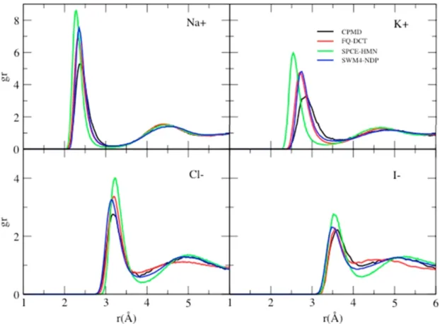
4.4 Radial Distribution Function . . . 53
4.5 Hydrogen Bond Kinetics . . . 54
4.5.1 Hydrogen Bond Kinetics Analysis . . . 54
4.5.2 Results . . . 55
4.6 Structral Makers and Structral Breakers . . . 55
4.7 Conclusion . . . 56
REFERENCES . . . 58
CHAPTER 5: WATER DIFFUSIVITY IN AQUEOUS IONIC SOLUTIONS: MD WITH CHARGE TRANSFER . . . 60
5.1 Introduction . . . 60
5.2 Computational Setups . . . 60
5.3 Potential of Mean Force for NaCl and KCl . . . 62
5.4 Charges on Ions and Charge Distribution among Water Molecules . . . 63
5.5 Detailed Analysis of Water Diffusion Coefficient . . . 65
5.6 Conclusion . . . 67
CHAPTER 6: POTENTIAL OF MEAN FORCE IN NACL SOLUTION: FIRST-PRINCIPLES MD WITH ADVANCED EXCHANGE CORRELATION
AP-PROXIMATIONS . . . 72
6.1 Introduction . . . 72
6.2 Two Advanced Functionals: SCAN andωB97X-V . . . 72
6.3 Computational Setups . . . 73
6.4 Liquid Water Properties at 300K . . . 76
6.5 Potential Energy Curve of NaCl in Vacuum . . . 78
6.6 Potential of Mean Force for NaCl in Water . . . 80
6.7 Inter-ion Water Structures along the Ion Separation . . . 82
6.8 Charges on Na and Cl Ions . . . 84
6.9 Charge Transfer and Polarization of Water Molecules . . . 85
6.10 Conclusion . . . 87
REFERENCES . . . 89
CHAPTER 7: DEVELOPMENT OF NEW ACKS2 MODEL FOR DESCRIBING CHARGE TRANSFER EFFECTS . . . 92
7.1 Density Functional Theory Derived Linear Response Polarizable Force Fields . . . 92
7.2 The ACKS2 Formula . . . 93
7.2.1 The EEM Formula . . . 93
7.2.2 The ACKS2 Formula . . . 94
7.2.3 The ACKS2 Formula with Atomic Dipole Included . . . 97
7.3 Examples . . . 100
7.3.1 Parameters Fitting . . . 100
7.3.2 Single Water Molecule . . . 101
7.3.3 20 Water Clusters . . . 102
7.3.4 Cl− with 30 Water Clusters . . . 105
7.4 Conclusion . . . 106
REFERENCES . . . 108
CHAPTER 8: CONCLUSION . . . 109
APPENDIX A: REPTATION QUANTUM MONTE CARLO ON NA-CL DIMER 113
A.1 Quantum Monte Carlo Methods . . . 113
A.1.1 Variational Monte Carlo . . . 113
A.1.2 Diffusion Monte Carlo . . . 114
A.1.3 Reptation Monte Carlo . . . 116
A.2 charge transfer in Na-Cl dimer . . . 116
A.2.1 Introduction . . . 116
A.2.2 Computational Methods . . . 116
A.2.3 Results . . . 117
A.2.4 Conclusion . . . 121
REFERENCES . . . 122
APPENDIX B: META-GGA SCAN IMPLEMENTATION . . . 123
B.1 Planewave implementation of SCAN metaGGA . . . 123
B.2 Norm-conserving pseudopotential for SCAN meta-GGA . . . 125
B.2.1 Atomic Kohn-Sham equation . . . 125
B.2.2 Troullier-Martins scheme for metaGGA pseudopotentials . . . 126
B.3 Examples of SCAN functional with planewave pseudopotential method . . . 128
B.3.1 Crystalline silicon and germanium . . . 129
B.3.2 Physisorption of water molecule on graphene . . . 132
B.3.3 Liquid water in different temperatures . . . 133
LIST OF FIGURES
1.1 (a) a picture of the earth mostly covered by the sea, (b) a schematic picture of the body to show the ratio of water in the body (c) a picture showing evidence of the
existence of salty water on Mars. . . 1
1.2 Two pioneer scientists in the field of aqueous solutions (a) Franz Hofmeister (b) Svante Arrhenius . . . 2
1.3 (a) We use mathematical formulas and computer programs to perform molecular dynamics simulations, (b) We are able to see each atom in molecular dynamics simulations . . . 3
2.1 A modern version of Hofmeister series . . . 7
2.2 Specific ion effects on water diffusivity . . . 8
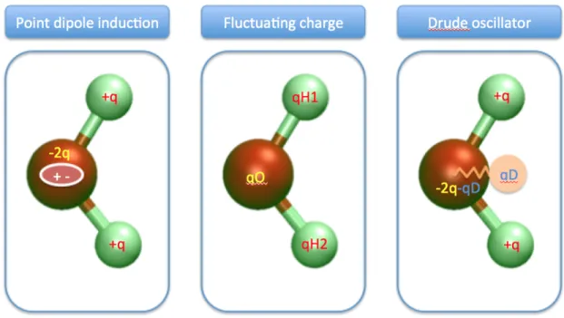
2.3 Schematic plots of three types of mostly used polarizable models . . . 11
3.1 Perdew’s Jacob’s ladder of density functional approximations to the exchange-correlation functional[22] . . . 26
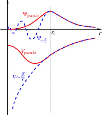
3.2 A schematic plot of the pseudopotential and pseudo-wavefunction compared to the exact Coulomb potential and wavefunction . . . 32
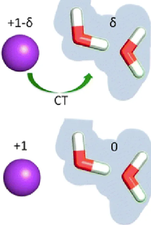
3.3 A schematic plot of charge transfer effect . . . 34
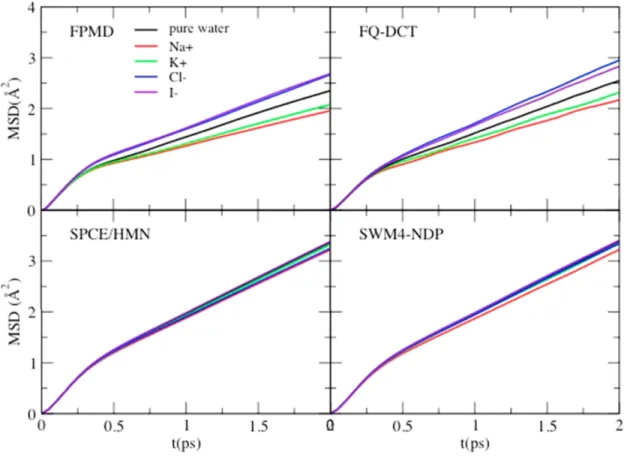
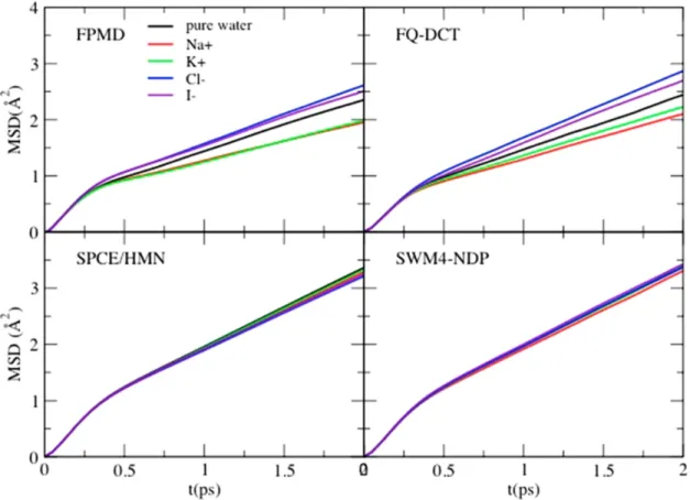
4.1 Mean square displacement of water in different ion-water systems . . . 50
4.2 Mean square displacement of water in different ion-water systems inside the first solvation shell of an ion . . . 51
4.3 Mean square displacement of water in different ion-water systems outside the first solvation shell of an ion . . . 52
4.4 Ion-water oxygen radial distribution functions in ion-water systems . . . 54
5.1 potential of mean force (PMF) in NaCl solution as a function of cation-anion separation distance calculated by classical molecular dynamics (MD) with FQ-DCT and SPCE-HMN models compared to First-Princples Molecular Dynamics (FPMD) simulations. THe shaded regions indicate the error bars estimated for FPMD curves . . . 63
5.2 PMF in KCl solution as a function of cation-anion separation distance calculated by classical MD with FQ-DCT and SPCE-HMN models compared to FPMD simulations. THe shaded regions indicate the error bars estimated for FPMD curves . . . 64
5.4 Ratio of the diffusion coefficient of water in ionic aqueous solution to that of pure water as a function of the salt concentration for NaCl (left) and for KCl (right). Black lines are for experimental values taken from Ref. 11, brown lines are for experimental values taken from Ref. 10, red lines are for classical MD simulations with FQ-DCT model, and blue curves are for simulations using the classical permanent charges force field (PQFF) model (specifically SPCE-HMN model). . . 67
5.5 Ratio of the water diffusion coefficient in the ionic aqueous solutions and the diffusion coefficient in pure water (D/D0) calculated for different spatial regions. (1) In the
first shell of water around N a+/K+. (2) In the first shell of water aroundCl−. (3) In the overlap region of first shells around N a+/K+ and Cl−. (4) Outside of the first shell of N a+/K+ and Cl−. The ratio of the average diffusion coefficient to the diffusion in pure bulk water is also shown (all). . . 68
6.1 The potential energy difference from MP2 result for the ωB97X-V functional with and without ADMM method. The results for the PBE, revPBE, PBE0, BLYP and RPA exchange correlation functionals are also shown . . . 74
6.2 The Oxygen-oxygen radius distribution function calculated from FPMD simulations based on the strongly constrained and appropriately normed (SCAN) meta-GGA functional. The comparison between the planewave (PW) simulation using the CPMD code and the Gaussian and planewave (GPW) simulation using the CP2K code is shown. The comparison between using the SCAN pseudopotential and the PBE pseudopotential is also shown for the PW simulations. . . 75
6.3 The potential of mean force calculated for Na-Cl in water at 300K with the SPC/F w/ HMN force field in classical molecular dynamics simulations with different integration time step size . . . 76
6.4 The oxygen-oxygen radial distribution functionsgOO(r) for pure liquid water
simu-lation at 300K , with SCAN, ωB97X-V, and PBE exchange correlation functionals. The MP2 result taken from ref. [25] by Monte Carlo simulation at 295K with the density of 1.02 g/cm3 is shown fro comparison. The experimental result from X-ray diffraction data is taken from ref [26] . . . 77
6.5 Distributions of molecular dipole moment magnitude for individual water molecules with SCAN,ωB97X-V, and PBE exchange correlation functionals. Maximally-localized Wannier functions are used to obtained the dipole moments on each water molecules 78
6.6 The potential energy curve of isolated Na-Cl pair in vacuum by MP2 and the CCSD(T) calculations with the aug-cc-pVTZ Gaussian basis set. The inset shows the energy difference between the MP2 and the CCSD(T) results . . . 79
6.7 (left) Potential energy curve of an isolated Na-Cl dimer in vacuum as a function of the separation distance according to several different exchange correlation functionals. The separation distance of 6 Åis used to align the curves for the comparison. The MP2 and theωB97X-V results are on top of each other at this scale. (Right) Deviations from the MP2 curve as a function of the separation distance . . . 79
6.8 The potential energy difference from the MP2 result forN a−H2O and Cl−H2O
interactions for theωB97X-V, SCAN, PBE, PBE0, BLYP, PBE-D3, and PBE0-D3 exchange correlation functionals . . . 80
6.10 (a) Two different types of water molecules that are involved in bridging Na and Cl ions. Relative counts for the two types of bridging water for the two types of bridging water molecules as a function of the Na-Cl separation distance for the MD simulations based on (b) SPC/F-HMN force field, (c) PBE XC, (d) ωB97X-V XC (e)SCAN XC 83 6.11 Averaged charge by Bader analysis for Na(left) and Cl(right) as a function of the
Na-Cl separation distance in the FPMD simulations. The shaded areas indicate the statistical error bars estimated for FPMD results with 400 equally-sampled snapshots taken from the FPMD trajectories. . . 84
6.12 (Left) Average Charges on individual water molecules around Na-Cl ion pair at three different Na-Cl separation distances. For example, the green regions indicate where the water molecules are likely more negatively charges. The red and the blue circles indicate where the Na and Cl ion is located, respectively. The distribution is averaged in the circular direction around the Na-Cl axis. (Right) Averaged charge on individual water molecules that are shared in the first solvation shells of Na and Cl ions as a function of the Na-Cl separation distance. The electron density was calculated on the 400 equally-sampled snapshots from the FPMD simulation trajectory for each XC functional, then Bader partitioning is performed to quantify the electron charge on each water molecule. . . 85
6.13 (Left) Averaged dipole magnitude of individual water molecules as a function of the Na-Cl separation distance in the FPMD simulations. Maximally-localized Wannier functions method is used to calculate the dipole moment of individual water molecules from the Kohn-Sham wavefunctions. (Middle) Averaged dipole magnitude for only the water molecules that were shared in the first solvation shells of both Na and Cl ions. (Right) Snapshots of the water molecules from the FPMD simulation, with and without a nearby Na ion. Hydrogen bonds are indicated by blue dashed lines. . . . 86
7.1 An example structure of water cluster with 20 water molecules . . . 103
7.2 The correlation plot between polarizable moments of ACKS2 and ACKS2-DIPOLE versus SWM4-NDP, SWM6, and FQ-DCT . . . 104
7.3 The correlation plot between dipole moments of ACKS2, ACKS2-DIPOLE, SWM4-NDP, SWM6, and FQ-DCT vs B3LYP DFT calculation . . . 105
7.4 An example structure of Cl− in 30 water molecules cluster . . . 106 7.5 The correlation plot of charges on Cl between, ACKS2, ACKS2-DIPOLE, FQ-DCT
and FQ-DCT . . . 107
7.6 The charge on the H2O molecules in the first solvation shell of Cl− . . . 107
A.1 electron distribution between Na-Cl dimer . . . 116
A.2 The amount of charge transfer between Na and Cl atoms as a function of the separation distance. Bader analysis was used for the charge partitioning. All the calculations here are performed with Gaussian basis set . . . 118
A.3 Charge transfer between Na and Cl atoms for different Na-Cl separation distances in HF and DFT calculations with various XC approximations . . . 119
A.5 Absolute total energies from RMC calculations with fermion nodes from HF and DFT calculations with various XC approximations for different Na-Cl separation distances. The filled squares indicate the fermion node that yields the lowest energy for a given separation distance. . . 120
A.6 Absolute total energy change as a function of Na-Cl separation distance in RMC calculations with fermion nodes from HF and DFT calculations with various XC approximations for different Na-Cl separation distances. . . 121
B.1 Convergence of the total energy of the crystalline silicon in the semiconducting diamond phase with respect to the planewave cutoff. The upper line (in black) is for the SCAN functional and the lower line (in red) is for the PBE functional. . . 129
B.2 Convergence of the total energy of the crystalline germanium in the semiconducting diamond phase with respect to the planewave cutoff. The upper line (in black) is for the SCAN functional and the lower line (in red) is for the PBE functional. . . 130
B.3 Convergence of the total energy of the crystalline silicon in the semiconducting diamond phase with respect to the FFT grid point. The upper line (in black) is for the SCAN functional and the lower line (in red) is for the PBE functional. . . 131
B.4 Convergence of the total energy of the crystalline germanium in the semiconducting diamond phase with respect to the FFT grid point. The upper line (in black) is for the SCAN functional and the lower line (in red) is for the PBE functional. . . 132
B.5 The band structure of the crystalline silicon in the semiconducting diamond phase, calculated using the SCAN functional (black) and the PBE functional (red). The SCAN functional result with the PBE functional PP is shown in blue. The generalized Kohn-Sham (gKS) equation is solved to obtain the eigenvalues in the case of the SCAN functional (details see text). The band structures were aligned such that the valence band maximum is set at 0 eV. . . 133
B.6 The band structure of the crystalline germanium in the semiconducting diamond phase, calculated using the SCAN functional (black) and the PBE functional (red). The SCAN functional result with the PBE functional PP is shown in blue. The generalized Kohn-Sham (gKS) equation is solved to obtain the eigenvalues in the case of the SCAN functional (details see text). The band structures were aligned such that the valence band maximum is set at 0 eV. . . 134
B.7 (a) Convergence of the adsorption energy for the water molecule physisorbed on the graphene sheet as a function of the planewave cutoff. The black curve shows the results using the default FFT grid using a particular FFT routine (FFTW code), and the red curve shows the results that are converged with respect to the FFT grid. (b) Total energies of adsorbed structure and isolated structure of water on graphene, along with adsorption energy as a function of the FFT grid density. The planewave cutoff of 60 Ry was used and the default FFT grid was used as the reference for FFT grid density (FFT grid density = 1). . . 135
B.8 The adsorption energy of a single water molecule on the graphene sheet as a function of the separation distance. The use of the PBE pseudopotential in the SCAN calculation did not change the SCAN result, and thus not shown. RPA, LDA, PBE, PBE0, and DMC (indicated by a) values are taken from Ref. [10] and shown for comparison. See text for details. . . 136
B.10 Radial distribution function for Oxygen-Oxygen in liquid water at 260K to 400K with SCAN functional . . . 138
LIST OF TABLES
4.1 Ratio of Diffusion Coefficients (D/D0) in Ion-water systems calculated with fluctuating
charge with discrete charge transfer (FQ-DCT), Density Functional Theory (DFT), SPC/E-HMN, and SWM4-NDP models, after each model name we list the length of the simulations. In the parentheses are the statistical uncertainties given by the standard deviation of the mean. . . 51
4.2 Properties of Bulk Neutral Water and Water with Small Charge on Each Water Molecule Calculated Using the FQ-DCT Model, hqOi,hqHi are the average charge on oxygen and hydrogen atoms,hµi is the average dipole moment of water molecules (Debye). D is the diffusion coefficient of water ( 10−9m2s−1). D/D0 is the relative
diffusion coefficient. . . 53
4.3 Hydrogen Bond Kinetics Constants for FQ-DCT, SWM4-NDP, and SPC-E/HMN Models, k is the reaction rate for hydrogen bond breaking, k’ is the reaction rate for the reverse reaction, and τHB is the lifetime of hydrogen bonds . . . 56
5.1 Simulation cell size and the number of water molecules and ions in the simulations at different salt concentrations . . . 61
5.2 The Lennard-Jones well-depth and radius, and the Drude charge and polarizability parameters for ions. . . 62
5.3 Charge transfer, electrostatic damping, and the Lennard-Jones combining rule param-eters for ion pairs and ion-water interactions . . . 62
5.4 Comparison of exchange-correlation (XC) functionals in DFT calculations for calcu-lating charges on cations and anions of NaCl and KCl in water, obtained using Bader analysis. . . 65
6.1 Locations of free energy minima and transition states, as well as key energetic quantities (in kcal/mol) from the potential of mean force as a function of the Na-Cl separation distances in water, according to different potential energy descriptions. CIP: Na-Cl distance for the contact ion pair, TS: Na-Cl distance for the transition state, SSIP: Na-Cl distance for the solvent separated ion pair,Ub: Free energy barrier
from CIP to SSIP, ∆CIP−SSIP: Free energy difference between CIP and SSIP. The
values in parentheses of SSIP indicate multiple possible SSIP locations. The values in parentheses forUb and∆CIP−SSIP indicates the statistical uncertainty for the free
energy values. a. ref [30] b. ref [29] . . . 82
7.1 parameters for ACKS2 and ACKS2-DIPOLE model, the energy in units of eV, length in units of Å, charge in units of electron charge . . . 101
7.2 The polarizabilities and dipole moment of single water molecule from SPC-FQ, TIP4P-FQ, FQ-DCT, ACKS2, ACKS2-DIPOLE models. The value from experiment is also listed for comparison . . . 102
7.3 The polarizabilities and dipole moment of single water molecule from SPC-FQ, TIP4P-FQ, FQ-DCT, ACKS2, ACKS2-DIPOLE models. The value from experiment is also listed for comparison . . . 103
B.2 Bandgaps (eV) of crystalline silicon and germanium in the semiconducting diamond phase. . . 131
LIST OF ABBREVIATIONS
ACKS2 Atom-Condensed Kohn-Sham approximation to second order. 39, 40, 94 ADMM auxiliary density matrix method. 74
BO Born-Oppenheimer. 35, 36
CIP contact ion pair. 75, 80
CPE chemical potential equalization. 10, 34–40, 94, 102 CPMD Car-Parrinello molecular dynamics. 37
CT charge transfer. 36, 37
DFT Density Functional Theory. xvii, 9, 10, 12, 35, 51
ECCR electronic continuum correction with rescaling. 68
FF force field. 9–13, 60
FPMD First-Princples Molecular Dynamics. xii, xiii, 49, 52, 56, 61–65, 72, 73, 75, 87 FQ fluctuating charge. 34
FQ-DCT fluctuating charge with discrete charge transfer. xvii, 49, 51
GPW Gaussian and planewave. xiii, 74, 75 GTH Goedecker-Teter-Hutter. 74
HF Hartree-Fock. 40, 73, 74
KS Kohn-Sham. 39, 73
PMF potential of mean force. xii, 62–64, 66, 72, 75, 76, 78, 80, 88 PW planewave. xiii, 74, 75
LIST OF PUBLICATIONS
[1] Yi Yao, Yosuke Kanai, and Max L Berkowitz. “Role of charge transfer in water diffusivity in aqueous ionic solutions”. In: The journal of physical chemistry letters 5.15 (2014), pp. 2711– 2716.
[2] Yi Yao, Max L. Berkowitz, and Yosuke Kanai. “Communication: Modeling of concentration dependent water diffusivity in ionic solutions: Role of intermolecular charge transfer”. In:The
Journal of Chemical Physics 143.24 (2015), p. 241101.
[3] Yi Yao and Yosuke Kanai. “Reptation quantum Monte Carlo calculation of charge transfer: The Na–Cl dimer”. In: Chemical Physics Letters 618 (2015), pp. 236–240.
[4] Kyle G Reeves, Yi Yao, and Yosuke Kanai. “Electronic stopping power in liquid water for protons andα particles from first principles”. In:Physical Review B 94.4 (2016), p. 041108. [5] Kyle G Reeves, Yi Yao, and Yosuke Kanai. “Diffusion quantum Monte Carlo study of martensitic
phase transition energetics: The case of phosphorene”. In:The Journal of chemical physics
145.12 (2016), p. 124705.
[6] Yi Yao and Yosuke Kanai. “Plane-wave pseudopotential implementation and performance of SCAN meta-GGA exchange-correlation functional for extended systems”. In:The Journal of
chemical physics 146.22 (2017), p. 224105.
[7] Yi Yao and Yosuke Kanai. “Free Energy Profile of NaCl in Water: First-Principles Molecular Dynamics with SCAN and ωB97X-V Exchange Correlation Functionals”. In: Journal of
Chemical Theory and Computation 14.2 (2018), pp. 884–893.
[8] Dillon C Yost, Yi Yao, and Yosuke Kanai. “Examining real-time time-dependent density functional theory nonequilibrium simulations for the calculation of electronic stopping power”.
CHAPTER 1: INTRODUCTION
1.1 Aqueous Ionic Solutions
In the environment and also in the human body, we can easily find the most abundant liquid on
earth – water. Instead of pure water, salt water – an aqueous ionic solution – forms the majority.
70% of earth’s surface is covered by the ocean. In the ocean, seawater on average has a salinity of
approximately 3.5%, meaning 35 grams of salts (mostly sodium chloride) per liter[1]. Beyond Earth,
on Mars for example, scientist have discovered flows of condensed aqueous ionic solutions[2][3]. In
addition, aqueous ionic solutions make up 60% of the human body, existing in almost all parts of
the body like cells, blood, brain and so on[4].
Figure 1.1: (a) a picture of the earth mostly covered by the sea, (b) a schematic picture of the body to show the ratio of water in the body (c) a picture showing evidence of the existence of salty water on Mars.
A large variety of aqueous ionic solutions exist, and they play important roles in biological
processes, industrial applications and scientific explorations due to their unique and valuable
the mechanisms of biological processes, such as digestion, signal transduction in the nervous
system and fluctuations of blood pressure[9][10][11]. Besides, taking advantage of the properties of
aqueous ionic solutions, people have made industrial applications like supercapacitors and water
desalination[6][7][8]. Additionally, in order to solve the longstanding scientific conundrum of the
origin of life, the properties of aqueous ionic solutions and how they interact with building blocks of
life need to be understood[12][13]. Thus, to understand the properties of aqueous ionic solution is
one typical question in the field of physical chemistry.
As one of the most classic physical chemistry systems, aqueous ionic solutions have already been
studied extensively even in college textbooks[14]. The beginning of the scientific study of aqueous
ionic solutions is in the 19th century, when Franz Hofmeister discovered salt species-dependent
properties – the salt out effects of proteins[15]. His work of such effects initiated the field of
ion-specific effects. Other than ion-ion-specific effects, in the same period of time, Svante August Arrhenius
established the electrolytic theory of dissociation which states that when salts are solvated in a water
solvent, instead of single molecules, they will first break up into two types of charged particles, one
carrying positive charge and the other carrying negative charge[16]. Those particles with positive
charge are cations and those with negative charge are anions, and they are called ions in general.
This theory about ions won him the Nobel prize in chemistry back in 1903.
1.2 Molecular Dynamics Simulation as a Tool to Investigate Aqueous Ionic Solutions From the 19th century – time of Hofmeister and Arrhenius – up to the present day, the major way
to investigate aqueous ionic solutions is experiments. By experiments, Most macroscopic properties
of these solutions are easy to measure[17]. For example, people could view precipitation by naked
eyes; scientists, with simple instruments, could measure osmotic pressures and electrical conductivity
even back in the 19th century. Nonetheless, elucidating the detailed microscopic structure and
dynamics of aqueous ionic solutions from experiment is a challenge due to lack of ability to directly
view the structure of the liquid. Without these direct information, macroscopic observations are
hard to explain from their molecular origin. For this reason, debates remain on questions such as
the relative importance of direct ion-ion interactions and the ion-water interactions in the dynamics
of such solutions[18]. We need tools beyond experiments for a deep understanding of aqueous ionic
solutions.
One of such tools is Molecular dynamics simulations[19][20][21]. These simulation methods – as
a growing technique in physical chemistry – are built bottom-up from basic physical laws. Follow
the physical laws, especially Newton’s second law, computers are used to generate and record the
trajectories for all the atoms and molecules in the system. The trajectories are then used to help
understand the macroscopic properties of solutions[22].
Figure 1.3: (a) We use mathematical formulas and computer programs to perform molecular dynamics simulations, (b) We are able to see each atom in molecular dynamics simulations
as connected points. These points interact with each other by known physical interactions like
Coulomb interactions and bond interactions. These interactions are usually calculated by computers.
Computers are also used to propagate the points based on Newton’s second law resulting in
trajectories. After sufficiently long simulation trajectories are collected, we analyze them and infer
macroscopic properties from them using statistical mechanics principles. [22].
Hence, molecular dynamics simulations are an important research tool in modern physical
chemistry[23] and are becoming a standard method to investigate aqueous ionic solutions[24]. In the
background chapter, I will introduce molecular dynamics simulations for liquid water and aqueous
ionic solutions and how the methodology has advanced over the years. Then, in the theoretical
method chapter, I will document the approaches in the molecular dynamics simulations field that I
used in my research. The research results for several systems related to aqueous ionic solutions are
REFERENCES
[1] Karl E Schleicher and Alvin Bradshaw. “A conductivity bridge for measurement of the salinity of sea water”. In:ICES Journal of Marine Science 22.1 (1956), pp. 9–20.
[2] Lujendra Ojha et al. “Spectral evidence for hydrated salts in recurring slope lineae on Mars”.
In: Nature Geoscience 8.11 (2015), p. 829.
[3] Erik Fischer et al. “Experimental evidence for the formation of liquid saline water on Mars”.
In: Geophysical research letters 41.13 (2014), pp. 4456–4462.
[4] The water in you. url:https://water.usgs.gov/edu/propertyyou.html.
[5] Astrid Sigel and Helmut Sigel.Metal ions in biological systems. CRC Press, 1998.
[6] Guan Wu et al. “High-performance supercapacitors based on electrochemical-induced vertical-aligned carbon nanotubes and polyaniline nanocomposite electrodes”. In:Scientific Reports 7 (2017), p. 43676.
[7] David Cohen-Tanugi and Jeffrey C Grossman. “Water desalination across nanoporous graphene”.
In: Nano letters 12.7 (2012), pp. 3602–3608.
[8] Evelyn N Wang and Rohit Karnik. “Water desalination: Graphene cleans up water”. In:Nature
nanotechnology 7.9 (2012), p. 552.
[9] GI Sandle. “Salt and water absorption in the human colon: a modern appraisal”. In:Gut 43.2 (1998), pp. 294–299.
[10] Irene Gavras and Haralambos Gavras. “’Volume-expanded’hypertension: the effect of fluid overload and the role of the sympathetic nervous system in salt-dependent hypertension”. In:
Journal of hypertension 30.4 (2012), pp. 655–659.
[11] Pierre Meneton et al. “Links between dietary salt intake, renal salt handling, blood pressure, and cardiovascular diseases”. In:Physiological reviews 85.2 (2005), pp. 679–715.
[12] Bruce Damer and David Deamer. “Coupled phases and combinatorial selection in fluctuating hydrothermal pools: A scenario to guide experimental approaches to the origin of cellular life”. In: Life 5.1 (2015), pp. 872–887.
[13] Bruce Damer. “A field trip to the Archaean in search of Darwin’s warm little pond”. In:Life
6.2 (2016), p. 21.
[14] Peter Atkins et al.Physical Chemistry: Thermodynamics, structure, and change. Macmillan Higher Education, 2014.
[15] Franz Hofmeister. “To the theory of the effect of salt”. In:Archive for Experimental Pathology
and Pharmacology 25.1 (1888), pp. 1–30.
[16] Svante Arrhenius. “Development of the theory of electrolytic dissociation”. In:Nobel Lecture
[17] William M Haynes.CRC handbook of chemistry and physics. CRC press, 2014.
[18] Werner Kunz. “Specific ion effects in colloidal and biological systems”. In:Current Opinion in
Colloid & Interface Science 15.1-2 (2010), pp. 34–39.
[19] Berni J Alder and T E Wainwright. “Studies in molecular dynamics. I. General method”. In:
The Journal of Chemical Physics 31.2 (1959), pp. 459–466.
[20] A Rahman. “Correlations in the motion of atoms in liquid argon”. In:Physical Review 136.2A (1964), A405.
[21] Frank H Stillinger and Aneesur Rahman. “Improved simulation of liquid water by molecular dynamics”. In:The Journal of Chemical Physics 60.4 (1974), pp. 1545–1557.
[22] Michael P Allen and Dominic J Tildesley.Computer simulation of liquids. Oxford university press, 2017.
[23] Wilfred F van Gunsteren and Herman JC Berendsen. “Computer simulation of molecular dynamics: Methodology, applications, and perspectives in chemistry”. In:Angewandte Chemie
International Edition 29.9 (1990), pp. 992–1023.
[24] Yizhak Marcus. “Effect of ions on the structure of water: structure making and breaking”. In:
CHAPTER 2: BACKGROUND
2.1 Specific Ion Effects and the Hofmeister Series
The study of specific ion effects is pioneered by the work of Franz Hofmeister about 120 years ago,
where he ranked a series of salts based on their abilities to precipitate proteins and mineral oxides
and so on[1]. After that, many other properties have also been used to rank the salt series. Nowadays
we usually refer these series as the Hofmeister series[2][3][4]. Though useful, the Hofmeister series
are not always consist with each other, and the origin of such series remain unclear. Depending on
the property used to order the Hofmeister series, the positions of different ions in the series may
vary. If the original Hofmeister series used, some properties could have a bell shape curve depend
on it or even reversed order[3]. These phenomena indicate the specific ion effect is not a single
effect. The combination of ion-water interactions, ion-ion interactions, and even ion-macromolecules
interactions together could lead to different order of Hofmeister series for different proteins or different
properties[4].
2.1.1 Specific Ion effects on Water Diffusivity
In the aqueous ionic solutions, the ions will influence the structure and dynamics of nearby water
molecules. One of the dynamical properties influenced by ions is the water diffusivity[5]. In general,
with the same amount of charge on the ion, the larger the ion is the larger the water diffusivity
around it. As shown in figure 2.2. However, the mechanism of how the ions influence the dynamics
Figure 2.2: Specific ion effects on water diffusivity
of water molecules remain unclear. What interactions influence the water dynamics is the first
question. Whether the ion-ion interaction important or not is another question. These questions
could be addressed easily if the molecular dynamics simulations could reproduce the diffusivity results.
Unfortunately, with most of the classical molecular dynamics simulations, the water diffusivity is not
even qualitatively correctly reproduced[5]. In my research, I used the advanced molecular dynamics
simulations to address this problem and gave my attempt to answer these questions.
In the next section, I will summarize the history and the state of arts for the molecular dynamics
2.2 Molecular Dynamics Simulations and First Principle Molecular Dynamics Simu-lations
Molecular dynamics is a simulation technique growing up with the advancing of the computer
technology[6]. It solves coupled equations of motion numerically. The solution results in trajectories
for molecules. Thermodynamical properties and dynamical properties can then be extracted from
such trajectories by statistical mechanical relationships.
During more than 60 years of development of molecular dynamics, the systems under investigation
go from simple to complex; the interaction potentials in the simulations go from coarse to accurate.
The first molecular dynamics simulations is performed by Alder and Wainwright to study the phase
transition for a hard sphere system in 1957[7]. The first molecular dynamics simulation for liquid
system is performed by Aneesur Rahman in 1964 for the study of the motions of atoms in the liquid
argon by simple Lennard-Jones potential[8]. Seven years later, Rahman and Stillinger published
the first ever molecular dynamics simulation of the liquid water with a point charge type model to
account for Coulomb interactions[9]. About 15 years later, in the year of 1986 Roberto Car and
Michele Parrinello merged the field of DFT and molecular dynamics simulation by includes the
electronic degrees of freedom in the molecular dynamics simulation which initiated the applications
of first principles molecular dynamics[10].
How to describe the interactions between atoms is the central part for molecular dynamics
simulations. These interactions are usually called force field (FF), which represent our knowledge
of potential energy surface of the system and is used to calculated the forces for propagating the
dynamical systems. The development of a good FF can be a challenge task. The method Rahman
and Stillinger used to describe the FF is usually refer as the empirical methods, where a certain
formula is chosen and fitted to expeirmental or electronic structure calculation properties. The
approach Car and Parrinello used is the so-called first principles approach. At each step of the
simulation, an electronic structure calculation is performed on the fly for the energy and forces.
In principle the underlying electronic structure is the more accurate the better. However, due to
the computational cost for exact electronic structure calculation is extremely high, approximate
methods are always used as the underlying theory which will limit its accuracy. Nowadays, DFT is
the most popular underlying electronic structure theory due to a good balance between accuracy
DFT, could be important in getting correct phenomena in the simulations[11][12].
The detailed discussion of the FF and DFT exchange correlation functionals could be found in
the next theoretical methods chapter. I will give a summary for the simulations of liquid water and
aqueous ionic solutions in the next section.
2.2.1 Molecular Dynamics Simulation of Liquid Water
In the pioneer work of Rahman and Stillinger, the FF is described by a combination of
Lennard-Jones potentials and electrostatic Coulomb potentials. The fixed charges are assigned on the four
fixed site of the water molecule, two hydrogen atoms and two lone pairs[9]. This type of FF is
the so-called fixed charge FF for water. Within this FF family, SPC[13], SPC/E[14], SPC/Fw[15],
TIP3P[16], TIP4P[16] are among the most popular ones which are widely used in the simulations
of biological systems like proteins. Due to the low computational cost of these models, they have
their value in large scale simulations such as biological systems and industrial applications. It is
interesting to note the recent development in this field, where data science and machine learning are
used to optimize the parameters for such force field and yield good liquid water properties even with
just a few parameters. TIP4P-FB[17], and OPC[18] are two promising models. For the self-diffusion
constant, with the TIP4P-FB FF, the simulation result is almost on top of the experimental value
among all the temperature range for liquid water.
Polarizable effect is the most common physical interaction beyond fixed charge models people
thought important to include in the simulations of liquid water[19][20]. Besides fixed charge Coulomb
interactions, this type of FF also includes the polarizable response of the water molecule to the
environmental electrostatic potentials (nearby molecules). Three techniques are usually used for
polarizable FF, the chemical potential equalization (CPE) model, the charge-on-spring model (Drude
model), and the induced dipole model. Among the three, Drude model is shown to be equivalent
to the induced dipole model[21]. TIP4P-FQ is a commonly used CPE FF for liquid water[22].
SWM4-DP and SWM4-NDP are among the popular FF within the family of Drude model [23] [24]
[25]. AMOEBA is an successful growing project for polarizable FF where high order of multipoles
and induced multipoles included[26]. The advantage of polarizable model over the fixed charge model
is usually significant for hetrogeneous systems, such as at the interface or next to some particles
Figure 2.3: Schematic plots of three types of mostly used polarizable models
Polarization is not the only physical response for the molecule to the environment. When two
particles or molecules get close to each other, some charge will be shared between the two. In the
theory of inter-molecular interaction, such effect is called charge transfer[27]. For bulk water and even
water at interfaces, this effects seems to be negligible[28]> However, for the water molecules next to
ions, this effect could lead to different results compared to fixed charge models[28][29]. Investigating
the charge transfer effects for water and ion is one of the major topic in my research.
Recent years, thanks to the development of data science and numerical optimization. Developing
force fields based on a large number of electronic structure theory calculations become feasible.
Several types of FF are developed not physical driven, but mathematical driven or data driven.
One example is the recent MB-pol model by Paesani[30][31][32][33][34]. The idea of many-body
expansion and the permutationally invariant polynomial are combined and fitted to a large amount
of highly precise electronic structure theory calculations. This model shows quite good agreement
with experimental results. The other example is the neural network FF, where the neural network is
used as a black box, local environment of each atom is used as the input for the black box and the
output is the energy on the potential energy surface. By using the neural network FF, a large amount
network FF could be trained and help extend the trajectory and get better statistics[35][36][37].
These developments in the force field by applying methods from data science might be criticized by
not physical driven, but on the other hand, pure mathematical model might help reduced the bias
introduced by physical intuition from scientists.
As we mentioned in the last section, the other approach for molecular dynamics simulation
is the first principles method. After each step of molecular dynamics simulations, the density
functional electronic structure theory calculations are performed to get the potential energies and the
forces[10]. The pioneer first principles molecular dynamics simulation of liquid water was published
in 1993 by Laasonen et al. with 32 water molecules and 1.5 ps trajectories collected[38]. The small
number of molecules and short trajectories indicate a large computational cost for first principle
molecular dynamics. Thanks to the computational power increasing in the last 25 years, the first
principles molecular dynamics simulation field grows a lot[39]. Today performing such simulations
with hundreds of molecules over hundreds of picoseconds is feasible with a supercomputer.
Not only the computer getting powerful, the techniques used in the first principles molecular
dynamics is also improved. For the numerical methods like basis sets, extrapolation scheme, new
ideas can always help improving the efficiency of the first principles molecular dynaimcs simulations.
For example, by using Gaussian basis sets instead of the planewave basis sets, usually a 10 times faster
simulation could be performed[40]. A better extrapolation scheme also help reduce the computational
cost by getting a better initial guess for the new electronic structure with the help of the former
electronic structures[41].
Also, as we discussed in the last chapter, the underlying theory used to perform electronic
structure calculation is usually DFT. The exchange correlation functional used in DFT also has its
improvement in these years[12]. For the simulation of liquid water, it improved from generalized
gradient approximation functionals to meta generalized gradient approximation functionals, and
hybrid functionals[42][43]. The explicitly inclusion of dispersion functional is another important
improvement in the simulation of liquid water[44]. In particularly, the recently developed SCAN
functional by Perdew and the functionals developed by Martin Head-Gordon both show good liquid
state properties compared to the older classical PBE functional[45][46][47].
remain to be solved.
2.2.2 Molecular Dynamics Simulation of Aqueous Ionic Solutions
Similar to pure liquid water simulations, for the aqueous ionic solutions simulations, different
kinds of models exist. For the classical FF simulations, it could be fixed charge models and polarizable
models[48][49]. For the first principles simulations, different type of exchange correlation functionals
usually yield different results[50]. Two reviews by Hitoshi Ohtaki and Tamas Radnal in 1993 and
Yizhak Marcus in 2009 has a good summary of the ion-water system simulations[51][52].
Though much has been done, new developments are still been made in the field of ion water
FF. One of the new important development principle is the screening effect of water to the ions,
when considered, the charge on ion is not integer number any more. When the charges are modified
the simulations match to the experimental results much better and the clustering problem in some
popular FF can be solved[53][54]. This method has a deep connection with our finding of charge
transfer effects.
Thanks to the increasing computing power, the simulations of ion-water systems can also be
performed at the level of first principles molecular dynamics level. Generalized gradient functionals
remain the most popular functional models for ion-water system. The importance of exact exchange
and dispersion correction is started to be explored in this area. In my Ph.D. work, I found the
importance of exact exchange is related to how good we need to describe the charge transfer effect.
If it is as importance as the charge transfer effect in vacuum, only exchange correlation functional
REFERENCES
[1] Franz Hofmeister. “To the theory of the effect of salt”. In:Archive for Experimental Pathology
and Pharmacology 25.1 (1888), pp. 1–30.
[2] MG Cacace, EM Landau, and JJ Ramsden. “The Hofmeister series: salt and solvent effects on interfacial phenomena”. In:Quarterly reviews of biophysics 30.3 (1997), pp. 241–277.
[3] Yanjie Zhang and Paul S Cremer. “Interactions between macromolecules and ions: the Hofmeis-ter series”. In:Current opinion in chemical biology 10.6 (2006), pp. 658–663.
[4] Pierandrea Lo Nostro and Barry W Ninham. “Hofmeister phenomena: an update on ion specificity in biology”. In: Chemical reviews 112.4 (2012), pp. 2286–2322.
[5] Jun Soo Kim et al. “Self-diffusion and viscosity in electrolyte solutions”. In:The Journal of
Physical Chemistry B 116.39 (2012), pp. 12007–12013.
[6] Michael P Allen and Dominic J Tildesley.Computer simulation of liquids. Oxford university press, 2017.
[7] BJ Alder and TEf Wainwright. “Phase transition for a hard sphere system”. In:The Journal
of chemical physics 27.5 (1957), pp. 1208–1209.
[8] A Rahman. “Correlations in the motion of atoms in liquid argon”. In:Physical Review 136.2A (1964), A405.
[9] Aneesur Rahman and Frank H Stillinger. “Molecular dynamics study of liquid water”. In:The
Journal of Chemical Physics 55.7 (1971), pp. 3336–3359.
[10] R Car and M Parrinello. “Unified approach for molecular dynamics and density-functional theory”. In: Physical review letters 55.22 (1985), p. 2471.
[11] Michiel Sprik, Jürg Hutter, and Michele Parrinello. “Ab initio molecular dynamics simulation of liquid water: Comparison of three gradient-corrected density functionals”. In:The Journal
of chemical physics 105.3 (1996), pp. 1142–1152.
[12] Miguel AL Marques, Micael JT Oliveira, and Tobias Burnus. “Libxc: A library of exchange and correlation functionals for density functional theory”. In:Computer Physics Communications
183.10 (2012), pp. 2272–2281.
[13] Herman JC Berendsen et al. “Interaction models for water in relation to protein hydration”. In:
Intermolecular forces. Springer, 1981, pp. 331–342.
[14] HJC Berendsen, JR Grigera, and TP Straatsma. “The missing term in effective pair potentials”.
In: Journal of Physical Chemistry 91.24 (1987), pp. 6269–6271.
[16] William L Jorgensen et al. “Comparison of simple potential functions for simulating liquid water”. In: The Journal of chemical physics 79.2 (1983), pp. 926–935.
[17] Lee-Ping Wang, Todd J Martinez, and Vijay S Pande. “Building force fields: an automatic, systematic, and reproducible approach”. In: The journal of physical chemistry letters 5.11 (2014), pp. 1885–1891.
[18] Saeed Izadi, Ramu Anandakrishnan, and Alexey V Onufriev. “Building water models: a different approach”. In: The journal of physical chemistry letters 5.21 (2014), pp. 3863–3871.
[19] Steven W Rick and Steven J Stuart. “Potentials and algorithms for incorporating polarizability in computer simulations”. In:Reviews in computational chemistry 18 (2002), pp. 89–146.
[20] Thomas A Halgren and Wolfgang Damm. “Polarizable force fields”. In: Current opinion in
structural biology 11.2 (2001), pp. 236–242.
[21] Jing Huang et al. “Mapping the Drude polarizable force field onto a multipole and induced dipole model”. In:The Journal of chemical physics 147.16 (2017), p. 161702.
[22] Steven W Rick, Steven J Stuart, and Bruce J Berne. “Dynamical fluctuating charge force fields: Application to liquid water”. In: The Journal of chemical physics 101.7 (1994), pp. 6141–6156.
[23] Guillaume Lamoureux, Alexander D MacKerell Jr, and Benot Roux. “A simple polarizable model of water based on classical Drude oscillators”. In:The Journal of chemical physics 119.10 (2003), pp. 5185–5197.
[24] Guillaume Lamoureux and Benot Roux. “Modeling induced polarization with classical Drude oscillators: Theory and molecular dynamics simulation algorithm”. In:The Journal of chemical
physics 119.6 (2003), pp. 3025–3039.
[25] Guillaume Lamoureux et al. “A polarizable model of water for molecular dynamics simulations of biomolecules”. In:Chemical Physics Letters 418.1-3 (2006), pp. 245–249.
[26] Jay W Ponder et al. “Current status of the AMOEBA polarizable force field”. In:The journal
of physical chemistry B 114.8 (2010), pp. 2549–2564.
[27] Anthony Stone.The theory of intermolecular forces. OUP Oxford, 2013.
[28] Alexis J Lee and Steven W Rick. “The effects of charge transfer on the properties of liquid water”. In: The Journal of chemical physics 134.18 (2011), p. 184507.
[29] Marielle Soniat and Steven W Rick. “The effects of charge transfer on the aqueous solvation of ions”. In:The Journal of chemical physics 137.4 (2012), p. 044511.
[30] Volodymyr Babin, Gregory R Medders, and Francesco Paesani. “Toward a universal water model: First principles simulations from the dimer to the liquid phase”. In:The journal of
[31] Gregory R Medders, Volodymyr Babin, and Francesco Paesani. “A critical assessment of two-body and three-two-body interactions in water”. In:Journal of chemical theory and computation
9.2 (2013), pp. 1103–1114.
[32] Volodymyr Babin, Claude Leforestier, and Francesco Paesani. “Development of a "first princi-ples" water potential with flexible monomers: Dimer potential energy surface, VRT spectrum, and second virial coefficient”. In: Journal of chemical theory and computation 9.12 (2013), pp. 5395–5403.
[33] Volodymyr Babin, Gregory R Medders, and Francesco Paesani. “Development of a "first principles" water potential with flexible monomers. II: Trimer potential energy surface, third virial coefficient, and small clusters”. In: Journal of chemical theory and computation 10.4 (2014), pp. 1599–1607.
[34] Gregory R Medders, Volodymyr Babin, and Francesco Paesani. “Development of a "first-principles" water potential with flexible monomers. III. Liquid phase properties”. In:Journal
of chemical theory and computation 10.8 (2014), pp. 2906–2910.
[35] Tobias Morawietz and Jorg Behler. “A density-functional theory-based neural network potential for water clusters including van der waals corrections”. In:The Journal of Physical Chemistry A 117.32 (2013), pp. 7356–7366.
[36] Tobias Morawietz et al. “How van der Waals interactions determine the unique properties of water”. In: Proceedings of the National Academy of Sciences 113.30 (2016), pp. 8368–8373.
[37] Tobias Morawietz and Jorg Behler. “A Full-Dimensional Neural Network Potential-Energy Surface for Water Clusters up to the Hexamer”. In: Zeitschrift fur Physikalische Chemie
227.9-11 (2013), pp. 1559–1581.
[38] Kari Laasonen et al. “"Ab initio" liquid water”. In: The Journal of chemical physics 99.11 (1993), pp. 9080–9089.
[39] Dominik Marx and Jurg Hutter. Ab initio molecular dynamics: basic theory and advanced
methods. Cambridge University Press, 2009.
[40] Joost VandeVondele et al. “Quickstep: Fast and accurate density functional calculations using a mixed Gaussian and plane waves approach”. In:Computer Physics Communications 167.2 (2005), pp. 103–128.
[41] Jiří Kolafa. “Time-reversible always stable predictor–corrector method for molecular dynamics of polarizable molecules”. In:Journal of computational chemistry 25.3 (2004), pp. 335–342.
[42] Luis Ruiz Pestana et al. “Ab initio molecular dynamics simulations of liquid water using high quality meta-GGA functionals”. In:Chemical Science 8.5 (2017), pp. 3554–3565.
[44] I-Chun Lin et al. “Importance of van der Waals interactions in liquid water”. In:The Journal
of Physical Chemistry B 113.4 (2009), pp. 1127–1131.
[45] Yi Yao and Yosuke Kanai. “Free Energy Profile of NaCl in Water: First-Principles Molecular Dynamics with SCAN and ωB97X-V Exchange Correlation Functionals”. In: Journal of
Chemical Theory and Computation 14.2 (2018), pp. 884–893.
[46] Mohan Chen et al. “Ab initio theory and modeling of water”. In:Proceedings of the National
Academy of Sciences 114.41 (2017), pp. 10846–10851.
[47] Narbe Mardirossian and Martin Head-Gordon. “ωB97X-V: A 10-parameter, range-separated hybrid, generalized gradient approximation density functional with nonlocal correlation, de-signed by a survival-of-the-fittest strategy”. In: Physical Chemistry Chemical Physics 16.21 (2014), pp. 9904–9924.
[48] Dominik Horinek, Shavkat I Mamatkulov, and Roland R Netz. “Rational design of ion force fields based on thermodynamic solvation properties”. In: The Journal of chemical physics
130.12 (2009), p. 124507.
[49] Haibo Yu et al. “Simulating monovalent and divalent ions in aqueous solution using a Drude polarizable force field”. In:Journal of chemical theory and computation 6.3 (2010), pp. 774–786.
[50] Takashi Ikeda, Mauro Boero, and Kiyoyuki Terakura. “Hydration of alkali ions from first principles molecular dynamics revisited”. In:The Journal of chemical physics 126.3 (2007), 01B611.
[51] Hitoshi Ohtaki and Tamas Radnai. “Structure and dynamics of hydrated ions”. In:Chemical
Reviews 93.3 (1993), pp. 1157–1204.
[52] Yizhak Marcus. “Effect of ions on the structure of water: structure making and breaking”. In:
Chemical reviews 109.3 (2009), pp. 1346–1370.
[53] Eva Pluharova et al. “Ab initio molecular dynamics approach to a quantitative description of ion pairing in water”. In:The journal of physical chemistry letters 4.23 (2013), pp. 4177–4181.
[54] Alan A Chen and Rohit V Pappu. “Parameters of monovalent ions in the AMBER-99 forcefield: Assessment of inaccuracies and proposed improvements”. In:The Journal of Physical Chemistry B 111.41 (2007), pp. 11884–11887.
CHAPTER 3: THEORETICAL METHODS
In this chapter, I will introduce the theoretical approaches and approximations used in this
research. The primary method used in our research is molecular dynamics – a computer simulation
method for the studying of the movements of molecules. During the molecular dynamics simulations,
we integrate the Newton’s equations of motion to get the trajectories of molecules. In this process,
the calculations of forces are essential. In our research, we calculated the forces with two flavors,
first principles molecular dynamics and force field molecular dynamics. When performing force field
molecular dynamics, we make models for molecules and assign some empirical interactions among
these molecules. The forces are calculated based on these models, i.e force fields. In the other
approach – the first principle molecular dynamics – instead of having some models for molecules,
we calculate the electronic structure of the system and derive forces from such calculations. In
theory, the law of nature for electronic structure is the Schrodinger’s equation. Although we know
the exact form of the Schrodinger’s equation, solving it exactly for realistic system is prohibitive
due to the complexity caused by the interactions among electrons. Approximations techniques are
developed to solve this equation. Density Functional Theory (DFT) is the most widely used one for
the electronic structure calculation. Although, as a theory, DFT is exact, in practice, approximate
exchange correlation functionals limit the accuracy of the calculations.
We will start by describing DFT and its approximations. Followed by the techniques for first
principles molecular dynamics. The theory of Quantum Monte Carlo – another more accurate
electronic structure theory – is introduced in the Appendix, and we used it to benchmark of charge
on NaCl dimer in vacuum. Our implementations and developments of force fields with charge
transfer effects included are also introduced. Finally, I will discuss about the methods for free energy
sampling as we used in our potential of mean force (PMF) calculations.
3.1 First-Principles Molecular Dynamics
experimental data is the most common way of describing the interactions. These functions could
be physical driven, i.e the interaction between molecules is separated to electrostatic interactions,
dispersion interactions, exchange interactions, and also induction interactions and charge transfer
interactions[2]. The common used Lennard-Jones potential plus point charges coulomb interaction
is one of the simplest example in this category[3]. The interaction functions can also be purely
mathematical driven. Manybody expansion force field, permutationally invariant polynomial basis
force field, and the recent neural network force field are all in this category[4][5][6]. These types
of functions are driven large attention these days due to the advance in data science and the
improvements in computing power which allowed people do large amount of calculations to get
enough reference data. After decades of research on the force fields, people have invented a zoo of
force fields. However, improvements are still needed. For example, the force fields with the usually
lacked charge transfer effects included is found to be important in certain circumstance by us[7][8].
Despite the successfulness of the force field molecular dynamics, existing of some kind of such
functional forms cause some disadvantages for them. For example, most force fields are made with
the assumption molecules remain the unchanged during the simulation. This made the force field
not suited for any kinds of chemical reaction. Though reactive force fields exist, the functional forms
are usually more complex and carefully adjustment of parameters for different systems are usually
needed[9]. The other situations are more practical, since force field development is not a simple task,
people usually go to the literature to find some already developed force fields instead of develop
them from scratch. Although, large amount of force field have been developed, not all system of
interest has some force field for it. Also, even if force fields for systems of interest are all exist. The
results calculated by different sets of force field are usually not comparable due to the different fitting
scheme. First principle molecular dynamics provide another way of doing molecular dynamics which
doesn’t have these problems[10].
The work flow of the classical molecular dynamics is first some functional forms are proposed
and fitted against some experimental or theoretical results, then using such functions to calculate
the forces at each timestep of molecular dynamics. The theoretical results are usually the energies
and forces got from electronic structure theory. The combination of electronic structure theory
and molecular dynamics started from Car and Parrinello results in the First-Principles molecular
electronic structure theory at each timestep of integrating the Newton’s equation of motion is the
basic idea of FPMD[11] In my works, I have used both methods due to the availability of them in
some specific codes.
The advantage of FPMD over the classical MD is due to the fact no functional form for
interactions are used. However, this doesn’t imply the calculation from first principle is exact. Since,
the Schrodinger’s equation for electrons is prohibitive expensive to solve, some kind of approximations
are always used for the calculation especially for FPMD where large amount of electronic structure
calculations are needed. Nowadays, The density functional method is the standard method for the
first principle molecular dynamics. Other kinds of electronic structure theory are also developed and
started to be used with molecular dynamics in recent years, for example MP2 method[12], and also
QMC method[13]. Here, I will focus on the DFT method, first.
In the following, I will introduce BOMD first. then, CPMD will be derived and discussed. After
that, the theory and approximations in density functional theory will be discussed.
3.1.1 Born-Oppenheimer Molecular Dynamics
Born-Oppenheimer molecular dynamics (BOMD) relies on the Born-Oppenheimer approximation.
The electronic structure can be calculated independent of the the atomic motion. In the molecular
dynamics calculation, at each time step, the forces are calculated by the time-independent Schrodinger
equation for the groundstate.
MIR¨I(t) =−∇Imin
Ψ0 hΨ0| ˆ
He|Ψ0i (3.1)
ˆ
HeΨ0=E0Ψ0 (3.2)
At the end of each step in BOMD, the electronic ground state are calculated and used to calculate
the forces on each atomic site.
BOMD is the naive way to implement the FPMD and it is introduced first. However due to
to perform FPMD. Nowadays, due to the continued improvement of the algorithms of solving the
self-consistent equations and the extrapolation methods, the efficiency of BOMD and CPMD is not
as large as years ago[10].
The very first first-principles molecular dynamics implemented by Car and Parrinello is called
Car-Parrinello molecular dynamics (CPMD) which is a clever way of solving the electronic structure
problem simultaneous with the dynamics propagation in molecular dynamics[11]
3.1.2 CPMD
The technique used by CPMD is the extended Lagrangian method. Car and Parrinello proposed
and implemented this method by extending the total Lagrangian of the MD system[11]. The fictitious
dynamics of the Kohn-Sham orbitals are added to the dynamics. The following Lagrangian is the
total Lagrangian used in the CPMD scheme:
LCP =
1 2
P
X
I=1
MIR˙2I+µ N
X
i=1
fi
Z
|φ˙i(r)|2dr−EKS[φi(r)](R) + N X i=1 fi N X j=1 Λij Z
φ∗i(r)φj(r)dr−δij
(3.3)
The four terms in the formula are the kinetic term for ions, the kinetic term for electrons, the
potential energy term, and the constraint added to the orbitals to ensure the orthonormalization of
the Kohn-Sham orbitals, respectively. fi are the occupation numbers associated with the orbitalsφi.
With the total Lagrangian of the system, the equation of motion for CPMD includes not only
the ion dynamics but also the electronic dynamics. The Euler-Lagrangian equations for both the ion
coordinates and the electronic orbitals are as follows:
d dt
∂L
CP
∂R˙I
=−∂LCP ∂RI
(3.4)
d dt
∂LCP ∂φ˙∗i(r)
!
=−δLCP
δφ∗i(r) (3.5)
The second equation involves functional derivatives because the orbitals are continuous scalar
fields.
of motion are obtained:
MIR¨I =−
∂EKS[φi(r)]
R ∂RI, (3.6)
µφ¨i(r, t) =−
δEKS[φi(r)]
δφ∗i(r) +
N
X
j=1
Λijφj(r, t) (3.7)
=−HˆKSφi(r, t) + N
X
j=1
Λijφj(r, t) (3.8)
where
ˆ
HKS =−~
2
2m∇
2+v
ext(r,R) +
Z ρ(r0) |r−r0|dr
0+µ
XC[ρ] (3.9)
is the Kohn-Sham Hamiltonian. TheΛis the Lagrange multiplier that ensures the orthonormality of
these Kohn-Sham orbitals.
The stationary solution for the CPMD should be equivalent to the self-consistent solution for
the Kohn-Sham equations. If the left-hand side of the equation (3.8) is removed, the Kohn-Sham
equations are recovered.
ˆ
HKSφi(r) = N
X
j=1
Λijφj(r). (3.10)
Here,φiis a unitary transform of the Kohn-Sham eigenfunctions. When the system is propagated,
this unitary transform is not valid any more. Nonetheless, the kinetic energy contribution to the
electronic energy is low and only departs slightly from the ground state. With the CPMD method,
the electronic states remain close to the Born-Oppenheimer surface during the propagation of the
total system. This is why CPMD is feasible.
Here we introduce the most common used underlying electronic structure thoery density functional
theory.
3.1.3 Density Functional Theory
Instead of many electron wavefuncionΨ(r1, r2, ...rn), as in the wavefunction methods, the density


![Figure 3.1: Perdew’s Jacob’s ladder of density functional approximations to the exchange-correlation functional[22]](https://thumb-us.123doks.com/thumbv2/123dok_us/8260588.2188491/47.918.173.747.462.1000/figure-perdew-density-functional-approximations-exchange-correlation-functional.webp)