Total Internal Reflection – Fluorescence Correlation Spectroscopy
(TIR-FCS): Application to the Study of Ligand – Receptor
Interactions
Punya Navaratnarajah
A dissertation submitted to the faculty of the University of North Carolina at Chapel Hill in partial fulfillment of the requirements for the degree of Doctor of
Philosophy in the Department of Biochemistry and Biophysics.
Chapel Hill 2012
ii ©2012
iii ABSTRACT
PUNYA NAVARATNARAJAH: Total Internal Reflection – Fluorescence Correlation Spectroscopy (TIR-FCS): Application to the Study of Ligand – Receptor Interactions
(Under the Direction of Nancy L. Thompson)
Ligand-receptor interactions are an integral part of cellular processes. Fully understanding these processes requires that the thermodynamic and kinetic parameters of ligand-receptor interactions be measured. Total internal reflection fluorescence microscopy combined with fluorescence correlation spectroscopy (TIR-FCS) can be used to characterize the interactions between a fluorescent ligand and surface-associated receptors. The overall objective of this work was to develop TIR-FCS so as to ease its implementation, and expand its application to the study of complex ligand-receptor systems.
Theoretical models describing ligand-receptor interactions measured by TIR-FCS depend on numerous parameters, which complicate the identification of optimal experimental conditions. Criteria, that, if satisfied, would yield autocorrelation curves containing significant information about the kinetics, were defined. Parameter space was systematically explored to identify experimental conditions that satisfy the criteria.
iv
ligand and receptors; while 2) nonfluorescent competitors (NC) compete with fluorescent species for receptors. To test these theoretical predictions, work was conducted to establish systems consisting of a NE and NC.
The pregnane X receptor (PXR), a transcription factor, peptides derived from co-activator and co-repressor proteins and a PXR ligand, rifampicin, were chosen to test NE theory. It was found that, contrary to the existing model of PXR action, rifampicin fails to allosterically enhance and reduce PXR’s affinity for co-activator and co-repressors, respectively. The biological significance of these results is discussed. These findings preclude the system from being used to test NE theory. As activators and co-repressors compete for PXR, the system can be used to test NC theory.
An IgG and Fc receptor, FcγRII, were initially chosen to test NC theory. Peptides derived from the antibody binding site on FcγRII were tested to identify those that compete with soluble FcγRII for surface-bound IgG. A poorly soluble peptide that
v
vi
ACKNOWLEDGEMENTS
I would like to express my profound gratitude and sincere appreciation to Dr. Nancy L. Thompson for her guidance and friendship during my graduate studies at UNC Chapel Hill. She created a unique learning environment that allowed me to become a well-rounded and independent scientist. Owing to her mentorship, I am a better researcher and experimentalist, scientific writer and communicator. Thank you, Nancy.
I would like to express my appreciation to my committee members Dr. Gerhard Meissner, Dr. Richard Wolfenden, Dr. Matthew Redinbo and Dr. Ken Jacobson. Dr. Redinbo, and a member of his lab, Dr. Laurie Betts, provided much helpful and crucial advice with regards the PXR project. Dr. Ken Jacobson kindly allowed me to take part in joint journal clubs between his lab and that of Dr. Klaus Hahn.
I owe a big thank you to Dr. Linda Spremulli whose door was always open to me. Her advice regarding my thesis work and graduate career were greatly appreciated.
vii
(Lawrence Lab) have always been unselfish with their time, helping me with the HPLC and mass spec, respectively.
I am immensely grateful to my friends in Chapel Hill, particularly Rukie, Dinuka, Laya and Jen, without whom graduate school would have been intolerable. Rukie, I am incredibly lucky to have had you both as a friend and roommate. I am going to miss you, your culinary inventions and the steady supply of good Sri Lankan tea. Dinuka, I look forward to you arranging all our reunions. Laya and Jen thank you for the endless hours of laughter, entertainment and forced trips to Glenwood Av.
viii
TABLE OF CONTENTS
LIST OF TABLES ...xii
LIST OF FIGURES ...xiii
LIST OF ABBREVIATIONS ...xiv
LIST OF SYMBOLS ...xvi
Chapter 1. Introduction...1
1.1 Overview...1
1.2 Total Internal Reflection Fluorescence Microscopy (TIRFM)...2
1.3 Fluorescence Correlation Spectroscopy (FCS)...3
1.4 Total Internal Reflection – Fluorescence Correlation Spectroscopy (TIR-FCS) ...4
1.5 Outline of Dissertation...6
1.5.1 Identifying Optimal Experimental Conditions for Measuring Surface Binding Thermodynamics and Kinetics using TIR-FCS...7
1.5.2 Establishing Biological Systems to Test TIR-FCS Theory Pertaining to Nonfluorescent Molecules ...8
1.5.2.1 Rifampicin – independent interactions between the pregnane X receptor ligand binding domain and peptide fragments of co-activator and co-repressor proteins ...9
1.5.2.2 Fc Receptor and IgG Interactions: A Test System for TIR-FCS ...10
ix
1.7 References...12
2. Identifying Optimal Experimental Conditions for Measuring Surface Binding Thermodynamics and Kinetics using TIR-FCS...16
2.1 Overview...16
2.2 Introduction...17
2.3 Theoretical Background...20
2.3.1 Total Internal Reflection with Fluorescence Correlation Spectroscopy ...20
2.3.2 Reaction Mechanism...23
2.3.3 Fluorescence Fluctuation Autocorrelation Function...24
2.3.4 Magnitude of the Fluorescence Fluctuation Autocorrelation Function ...25
2.3.5 Time Dependence of Ga(τ)...25
2.3.6 Time Dependence of Gs(τ)...26
2.4 Results...26
2.4.1 Measurement of K by Steady-State TIRFM...26
2.4.2 Criteria for TIR-FCS...28
2.4.3 Experimental Conditions that Meet the Criteria...30
2.4.4 Measurement of K by TIR-FCS...37
2.4.5 Measurement of kd, or kd and ka, by TIR-FCS...40
2.5 Discussion ...42
2.5.1 Summary of Results...42
2.5.2 Comparison with Experimental Results...44
2.5.3 Expanded Range...51
x
2.6 Acknowledgements...59
2.7 References...60
3. Rifampicin – independent interactions between the pregnane X receptor ligand binding domain and peptide fragments of co-activator and co-repressor proteins ...65
3.1 PXR as a Potential Test System for TIR-FCS...65
3.2 Overview...67
3.3 Introduction...68
3.4 Materials and Methods...70
3.4.1 PXR-LBD Cloning, Expression, Purification and Labeling...70
3.4.2 Co-regulator Peptide Synthesis and Fluorescence Labeling...73
3.4.3 Other Reagents...74
3.4.4 Sample Preparation...75
3.4.5 Fluorescence Microscopy...76
3.4.6 Steady-State Total Internal Reflection Fluorescence Microscopy ...77
3.4.7 Total Internal Reflection with Fluorescence Recovery After Photobleaching ...78
3.5 Results...78
3.5.1 Control Measurements...79
3.5.2 F-SRC-1/PXR-LBD Equilibrium Dissociation Constants Measured by Steady-State TIRFM ...81
3.5.3 F-SRC-1/PXR-LBD Dissociation Rate Constants Measured by TIR-FRAP ...85
3.5.4 SMRT/PXR-LBD Equilibrium Dissociation Constants Measured by Steady-State TIRFM ...90
xi
3.7 Acknowledgements ...104
3.8 References ...105
4. FcγRII and IgG Interactions: A Test System for TIR-FCS...111
4.1 Introduction...111
4.1.1 Theoretical Background...112
4.1.2 Model System...116
4.2 Materials and Methods...118
4.2.1 Cell Culture...118
4.2.2 Purification of sFcγRII...118
4.2.3 Purification of 1B7.11 Antibody...119
4.2.4 Fluorescence Labeling...119
4.2.5 Sample Preparation...120
4.2.6 TIRFM Instrumentation...121
4.2.7 Experiments ...122
4.3 Results ...123
4.3.1 Theoretical Work to Find Optimal Experimental Conditions...123
4.3.2 Experimental Work to Establish the Model System...125
4.3.2.1 1B7.11 was specifically immobilized on DNP-cap-DPPE – containing supported planar membranes ...126
4.3.2.2 F-sFcγRII binds specifically to membrane- bound 1B7.11 ...127
xii
4.4 Conclusion ...131
4.5 References ...133
5. Summary and Future Directions ...135
xiii
LIST OF TABLES
Table 2.1: Parameters Governing the Behavior of G(τ) ...29
Table 2.2: Criteria ...30
Table 2.3: Conditions for which Criteria A-E are Satisfied ...33
Table 2.4: Surface Site Densities for Lower Values of Gs(0) ...53
Table 2.5: Gs(0) Values for Different Surface Site Densities ...54
Table 2.6: Gs(0)/Ga(0) Values for Different Surface Site Densities ...55
Table 2.7: Rebinding Probabilities P for Different Surface Site Densities ...56
Table 3.1: F-SRC-1/PXR-LBD Equilibrium Dissociation Constants Measured by Steady-State TIRFM ...84
Table 3.2: Co-repressor/PXR-LBD Equilibrium Dissociation Constants Measured by Steady-State TIRFM ...92
xiv
LIST OF FIGURES
Figure 1.1: Through-Prism TIR-FCS ... 5
Figure 1.2: Fluorescence Fluctuation Autocorrelation Functions ... 6
Figure 1.3: IgG Dynamics ...7
Figure 2.1: TIR-FCS ... 22
Figure 2.2: Reaction Mechanism ... 24
Figure 2.3: Measurement of K by Steady-State TIRFM ... 28
Figure 2.4: Conditions Required for TIR-FCS ... 35
Figure 2.5: Measurement of K by using TIR-FCS ... 38
Figure 2.6: Measurement of kd, or kd and ka, by TIR-FCS ... 42
Figure 3.1: Domain Organization of PXR...70
Figure 3.2: Specificity of PXR-LBD Immobilization ...80
Figure 3.3: Representative F-SRC-1/PXR-LBD Binding Isotherm ... 82
Figure 3.4: Representative Fluorescence Recovery Curves ... 86
Figure 3.5: F-SRC-1/PXR-LBD Dissociation Rate Constants Measured by TIR-FRAP and Theoretical Probabilities of Rebinding ... 89
Figure 3.6: Representative Co-repressor Competition Data ... 92
Figure 4.1: Structure of IgG1 and extracellular region of FcγRII ... 117
Figure 4.2: Through-prism TIRFM... 121
Figure 4.3: Sample Autocorrelation Plots with a Significant Dependence on k-2 ... 124
Figure 4.4: Sample Autocorrelation Plots with No Significant Dependence on k-2 ... 125
Figure 4.5: Schematic of Experimental System ... 126
Figure 4.6: Binding of F-1B7.11 to DNP-cap-DPPE/DPPC Planar Membranes ... 127
xv
xvi
LIST OF ABBREVIATIONS
AF-2 activation function – 2 ATP adenosine triphosphate CCD charge-coupled device CHO Chinese hamster ovary DLS dynamic light scattering
DMEM Dulbecco’s modified eagle medium
DMF dimethylformamide
DMSO dimethyl sulfoxide DNA deoxyribonucleic acid DBD DNA binding domain
DNP-cap-DPPE 1,2-dipalmitoyl-sn -glycero-3-phosphoethanolamine-N-[6-[(2,4-dinitrophenyl)amino]hexanoyl]
DNP-G dinitrophenyl – glycine
DPPC 1,2-dipalmitoyl-sn-glycero-3-phosphocholine EDTA ethylenediaminetetraacetate
EGFP enhanced green fluorescent protein ELISA enzyme-linked immunosorbent assay
ER estrogen receptor
FCS fluorescence correlation spectroscopy FcγRII mouse Fc receptor
FITC fluorescein isothiocyanate
FRET fluorescence resonance energy transfer GR glucocorticoid receptor
xvii
HPLC high-performance liquid chromatography HRP horseradish peroxidase
IDM indomethacin
IgG immunoglobulin G
NCoR nuclear receptor co-repressor PBS phosphate buffered saline
PPAR peroxisome proliferator-activated receptor PXR pregnane X receptor
PXR-LBD ligand binding domain of the pregnane X receptor RID receptor interaction domain
RXR retinoid X receptor
SDS-PAGE sodium dodecyl sulfate polyacrylamide gel electrophoresis sFcγRII soluble, extracellular domain of FcγRII
SMRT silencing mediator for retinoid and thyroid hormone receptors SRC-1 steroid receptor co-activator – 1
SUV small unilamellar vesicle
TCEP tris(2-carboxyethyl)phosphine hydrochloride
TFP tetrafluorophenyl
TIR total internal reflection
xviii
LIST OF SYMBOLS
α angle on incidence
αc critical angle
A average concentration of fluorescent ligand in solution (Chapters 2 and 3)
B average density of unoccupied, nonfluorescent surface binding sites (Chapter 2)
C average density of bound, fluorescent surface binding sites (Chapter 2)
d depth of the evanescent wave
D solution diffusion coefficient of fluorescent molecules ε molar extinction coefficient
G(τ) fluorescence fluctuation autocorrelation function
Ga(τ) autocorrelation term related to diffusion through the evanescent wave
Gs(τ) autocorrelation term related to surface association/dissociation kinetics
h radius of the observation area in the sample plane defined by the pin hole
I0 intensity of incident light
K, K1, K2 equilibrium association constants for [fluorescent ligand (Chpater 2), fluorescent reporter-ligand (Chapter 4), nonfluorescent
competitor (Chapter 4)] and surface binding sites
Kd, Kd’ equilibrium dissociation constants for (SRC-1, co-repressor) and PXR (Chapter 3)
k1, k2 association rate constants for (fluorescent reporter-ligand, nonfluorescent competitor) and surface binding sites (Chapter 4) k-1, k-2 dissociation rate constants for (fluorescent reporter-ligand,
xix
ka, kd association, dissociate rate constants for fluorescent ligand and surface binding sites (Chapter 2)
koff dissociation rate constant for SRC-1 and PXR (Chapter 3) λ0 vacuum wavelength of incident light
Lc nonfluorescent competitor (Chapter 4) Lf fluorescent reporter-ligand (Chapter 4) n1 refractive index of glass medium n2 refractive index of aqueous medium
NB average number of unoccupied surface binding sites in the observation area (Chapter 2)
NC average number of occupied, fluorescent surface binding sites in the observation area (Chapter 2)
Rr rate of diffusion parallel to the sample plane through the observation area
Chapter 1
Introduction
1.1 Overview
A comprehensive mechanistic understanding of biochemical processes requires that the thermodynamic and kinetic parameters pertaining to the interaction of relevant biological molecules be measured. Several techniques, including isothermal calorimetry and surface plasmon resonance, allow for such measurements. A fluorescence microscopy-based technique, total internal reflection – fluorescence correlation spectroscopy (TIR-FCS), can also be used to study the thermodynamics and kinetics of interacting molecules. TIR-FCS and variations thereof have the advantage that that they are versatile and amenable to live cell imaging, yielding both thermodynamic and spatio-temporal information. The focus of the present work has been the development of TIR-FCS for its application towards the thermodynamic and kinetic characterization of fluorescent molecules in solution that reversibly interact with surface-bound, non-fluorescent molecules. In practical terms, this work facilitates the adoption of the technique to study the interaction between soluble ligands and membrane-bound receptors, as well as the interaction between soluble biological molecules where at least one of the interacting partners is amenable to surface-immobilization.
2
1.2 Total Internal Reflection Fluorescence Microscopy (TIRFM)
TIR-FCS combines two well established techniques, total internal reflection fluorescence microscopy (TIRFM) and fluorescence correlation spectroscopy (FCS). In TIRFM (1-3), evanescent illumination is used to specifically excite fluorescently labeled molecules that are in close proximity to a surface, usually an aqueous/glass interface. Briefly, when light traveling in a medium with refractive index n1 impinges on an interface with a lower refractive index (n2) medium, at an angle greater than the critical angle, αc, where
2 1
1sin n n
c
, (1.1)
the light is completely reflected back into the first medium in a process called total internal reflection. During TIR, a component of the incident light propagates parallel to the TIR interface and penetrates into the lower refractive index medium, where the intensity, I(z), decays exponentially with increasing distance, z, from the interface:
zd e I zI 0 . (1.2)
The depth, d, of this exponentially decaying evanescent wave is determined by the vacuum wavelength of the incident light, λ0, the angle of incidence, α, and refractive indices, n1 and n2:
2 2 2 2 1 0 sin
4 n n
d
. (1.3)
3
1.3 Fluorescence Correlation Spectroscopy (FCS)
As fluorescently labeled molecules diffuse in and out of the observation volume, the fluorescence signal fluctuates. The temporal pattern of these fluorescence fluctuations is altered if the molecules reversibly interact with surface binding sites, for instance, impeding their ability to freely diffuse. FCS (4-9) can be used to measure the temporal pattern of fluorescence fluctuations and, thereby, gain insight into the dynamics of the fluorescent species being studied. Towards this end, fluctuations in the
fluorescence signal, defined as the difference
F
t
between the instantaneousfluorescence, F(t), and the time-averaged fluorescence, F , are autocorrelated as a
function of the lag-time, , using the following equation:
2
F t F t F
G . (1.4)
The autocorrelation function, G
τ , is independent of the time, t, when the system ofinterest is at equilibrium. G
τ decays to zero as approaches infinity. The magnitudeof this function is inversely related to the average number of fluorescent molecules in the
observation volume. The rate of decay and shape of G
τ contain information about theprocesses that affect the pattern of fluorescence fluctuations, including photo-physical dynamics (e.g., triplet state kinetics), solution diffusion, association and dissociation with surface-binding sites, and/or enzyme kinetics.
4
autocorrelation functions with magnitudes large enough to be accurately measured, the average number of fluorescent molecules in the observed volume has to be small. Most FCS measurements are carried out with at most 100 fluorescent molecules in the observed volume. One way to reduce the average number of fluorescent molecules in the observation volume, other than by simply decreasing the concentration, is to reduce the size of the detection volume.
5
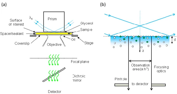
Figure 1.1: Through-Prism TIR-FCS. (a) A laser beam is totally internally reflected at a sample plane through a prism that is mounted on the stage of an inverted microscope. (b) An evanescent wave of depth d excites fluorescence, which is collected through the high-aperture objective and passed through a spectral filter to remove scattered evanescent light. The light is passed through a small aperture, placed at a back image plane of the microscope, before reaching a single-photon counting detector. The detector signal is processed using a computer with a correlator card and associated software. Reproduced with permission from J. Struct. Biol. 2009. 168, 95-106.
In TIR-FCS fluorescence fluctuations arising from fluorescent species that move in and out of the detection volume, undergo photophysics and/or reversibly associate with the surface are autocorrelated (Figure 1.2). Measured autocorrelation functions are fit to theoretical models derived for a given system, to obtain values of the parameters of interest. These theoretical autocorrelation functions take into account the optical arrangement of the excitation and emission pathways, as well as the processes giving rise to the observed fluorescence fluctuations. Many different theoretical models have been described in the literature: triplet state kinetics (18); diffusion in the evanescent field ( 20-24); ligand-receptor kinetics (25, 26); enzyme kinetics (27); cross-correlation TIR-FCS (28); and other situations (16, 17, 29, 30).
6
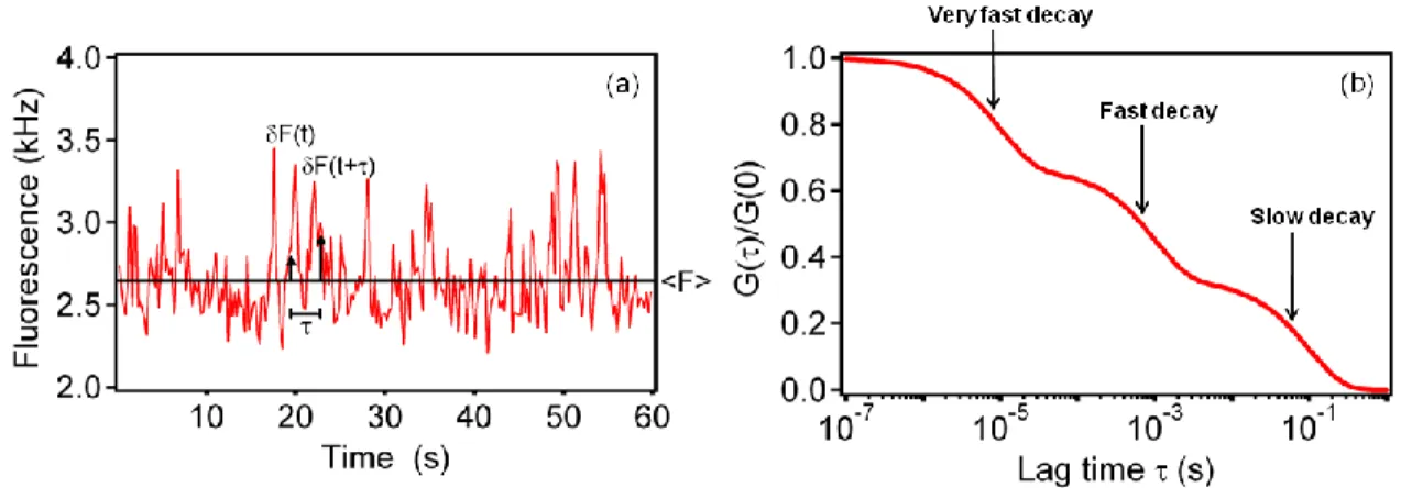
Figure 1.2: Fluorescence Fluctuation Autocorrelation Functions. (a) The fluorescence measured from the observation volume fluctuates with time as individual fluorescent molecules diffuse through the evanescent field, associate with and dissociate from surface binding sites, and/or undergo transitions between states with different detected fluorescence intensities. (b) The temporal fluorescence fluctuations are autocorrelated (see Eq. 1.4). This plot shows an idealized case in which three components with different characteristic rates are present in G(τ); e.g., a very fast decay arising from photophysics, a fast decay arising from free diffusion of the fluorescent molecules through the depth of the evanescent field, and a slow decay resulting from reversible association of the fluorescent molecules with surface sites. Reproduced with permission from Reviews in Fluorescence 2009; Geddes, CD, Ed.; Springer: New York; pp 345-380.
1.5 Outline of Dissertation
In the present work we are concerned with the extension of TIR-FCS to the study of ligand-receptor kinetics. This particular application of TIR-FCS was first demonstrated when the technique was used to examine the kinetics of the mouse Fc receptor, FcγRII, and an IgG (14). To conduct these measurements, FcγRII was
7
curves obtained for ligand-receptor interactions contained a long-time component that is absent when the fluorescence fluctuations arise due to diffusion alone (Figure 1.3).
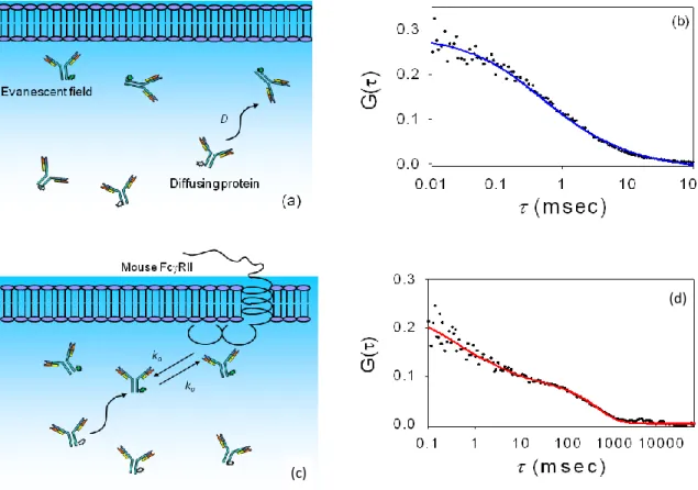
Figure 1.3: IgG Dynamics. (a) Schematic of antibody diffusion close to a supported planar membrane. Fluorophores within the evanescent wave are excited and fluoresce. (b) Representative TIR-FCS data and the best fit to an appropriate theoretical expression. The data are for a mixture of 10 nM Alexa448-labeled IgG, 1 μM unlabeled IgG and 10 mg mL-1 ovalbumin in phosphate-buffered saline close to surfaces coated with supported phospholipid bilayers. (c) Schematic of antibodies diffusing close to and reversibly associating with a supported planar membrane containing purified and reconstituted Fc receptors. The parameters
kaand kd are the association and dissociation rate constants, respectively. d) Representative
TIR-FCS data and the best fit to an appropriate theoretical expression. The data are for a mixture of 10 nM Alexa448-labeled IgG, 1 μM unlabeled IgG and 10 mg mL-1 ovalbumin in phosphate-buffered saline close to surfaces coated with supported phospholipid bilayers containing approximately 800 receptors per μm2
. Parts (a) and (c) are reproduced with permission from Reviews in Fluorescence 2009; Geddes, CD, Ed.; Springer: New York; pp 345-380. Parts (b) and (d) are reproduced with permission from Biophys. J. 2003. 85, 3294-3302.
1.5.1 Identifying Optimal Experimental Conditions for Measuring Surface Binding Thermodynamics and Kinetics using TIR-FCS
The theoretical model pertaining to ligand-receptor kinetics was extensively described by Lieto and Thompson (25). This work showed that numerous experimental
(d)
8
parameters, including the dimensions of the detection volume, concentration of fluorescent ligand and density of surface-bound receptors, affect the magnitude and shape of the autocorrelation curve. As a result, it is difficult to identify experimental conditions that will yield TIR-FCS curves that have high signal-to-noise ratios and contain significant information about the thermodynamic and kinetic parameters of interest. To address this difficulty, we defined criteria that, if satisfied, would yield autocorrelation curves that allow for successful measurement of equilibrium binding constants and rate constants. We then systematically explored the parameter space to identify experimental conditions that would satisfy the criteria. The work is geared to serve as a general guide to determine optimal experimental conditions for TIR-FCS measurements involving different biological systems and thereby ease the implementation of the technique. This work was outlined in a paper I co-authored (31) and is included in Chapter 2 of this dissertation.
1.5.2 Establishing Biological Systems to Test TIR-FCS Theory Pertaining to Nonfluorescent Molecules
9
I set out to implement two biological test systems, one containing a nonfluorescent enhancer and the other, a nonfluorescent competitor.
1.5.2.1 Rifampicin – independent interactions between the pregnane X receptor ligand binding domain and peptide fragments of co-activator and co-repressor proteins
For a test system containing a nonfluorescent enhancer, we chose a nuclear receptor, the pregnane X receptor (PXR), one of its co-activator proteins and an established ligand of PXR, rifampicin. PXR regulates the expression of drug metabolizing enzymes in a ligand-dependent manner (32). The existing model of nuclear receptor action states that upon binding agonists, nuclear receptors associate with co-activators, which in turn recruit downstream members of the cell’s transcription machinery. We thought to adopt a system in which the PXR agonist rifampicin would serve as a nonfluorescent enhancer and a fluorescently labeled peptide derived from the steroid receptor co-activator 1 (SRC-1) would serve as the fluorescent reporter. The PXR ligand binding domain (PXR-LBD) was in turn immobilized on fused silica microscope slides via a biotin – avidin linkage. As the interaction among PXR, its co-regulator proteins and agonists had not been biophysically characterized prior to this work, we used established techniques, TIRFM and TIRFM combined with fluorescence recovery after photobleaching (TIR-FRAP), to measure the thermodynamics and kinetics of the interaction between PXR-LBD and SRC-1 in the presence and absence of rifampicin. Contrary to expectations, rifampicin did not alter the affinity of PXR-LBD for SRC-1. Although the system could not be used to test TIR-FCS theory pertaining to nonfluroescent enhancers, the work strongly suggested that the mechanism of PXR action differed from that of other nuclear receptors. These findings were published in
10
As agonists are also thought to decrease the affinity of nuclear receptors for co-repressors (34-36), we used TIRFM to investigate the interaction between PXR-LBD and peptides derived from co-repressor proteins. Again, rifampicin did not alter the affinity of PXR-LBD for its co-repressors. However, as co-activator and co-repressor binding sites on nuclear receptors overlap significantly (37), co-activator and co-repressor peptides compete with each other to bind PXR-LBD. We thereby had a system with which to test the nonfluorescent competitor theory. In addition, PXR-LBD and its interacting partners could be used to test the experimental conditions (Chapter 2) that were predicted to yield informative autocorrelation curves with good signal-to-noise ratios.
1.5.2.2 Fc Receptor and IgG Interactions: A Test System for TIR-FCS To test the nonfluorescent competitor theory, we initially sought to use an IgG and its Fc receptor, FcγRII. Unlike PXR interactions, the interaction between antibodies
and their Fc receptors are well characterized (14). However, a known competitive inhibitor of IgG/FcγRII binding did not exist. We designed a system in which an IgG,
1B7.11, was immobilized on supported planar membranes via its antigen binding site. The soluble, extracellular portion of FcγRII (sFcγRII) was fluorescently labeled and
introduced into the aqueous medium between the microscope slide and cover slip. To obtain nonfluorescent competitors, we synthesized peptides fashioned from the antibody binding site on FcγRII (38, 39). One of these peptides was able to compete with sFcγRII
11 1.6 Summary
12 1.7 References
1. Simon, S. M. (2009) Partial internal reflections on total internal reflection fluorescent microscopy. Trends in Cell Biology 19, 661-668.
2. Axelrod, D. (2008) Total internal reflection fluorescence microscopy. Methods in Cell Biology 89, 169-221.
3. Schneckenburger, H. (2005) Total internal reflection fluorescence microscopy: technical innovations and novel applications. Current Opinion in Biotechnology 16, 13-18.
4. Fitzpatrick J. A. J., Lillemeier, B. F. (2011) Fluorescence correlation spectroscopy: linking molecular dynamics to biological function in vitro and in situ. Current Opinion in Structural Biology 21, 650 – 660.
5. Chiantia, S., Reis, J., Schwille, P. (2009) Fluorescence correlation spectroscopy in membrane structure elucidation. Biochimica et Biophysica Acta 1788, 225-233. 6. Chen, H., Farkas, E. R., Webb, W.W. (2008) In vivo applications of fluorescence
correlation spectroscopy. Methods in Cell Biology 89, 3-35.
7. Kolin, D. L., Wiseman, P. W. (2007) Advances in image correlation spectroscopy: Measuring number densities, aggregation states, and dynamics of fluorescently labeled macromolecules in cells. Cell Biochemistry and Biophysics 49, 141-164.
8. Haustein, E., Schwille, P. (2007) Fluorescence correlation spectroscopy: Novel variations of an established technique. Annu. Rev. Biophys. Biom. 36, 151-169. 9. Blom, H., Kastrup, L., Eggeling, C. (2006) Fluorescence fluctuation spectroscopy
in reduced detection volumes. Current Pharmaceutical Biotechnology 7, 51-66. 10. Thompson, N. L., Navaratnarajah, P., Wang, X. (2009a) Total internal reflection
with fluorescence correlation spectroscopy. Reviews in Fluorescence 2009; Geddes, CD, Ed.; Springer: New York; pp 345-380.
11. Thompson, N. L., Wang, X., Navaratnarajah, P. (2009b) Total internal reflection with fluorescence correlation spectroscopy: Applications to substrate-supported planar membranes. J. Struct. Biol. 168(1):95-106.
12. Thompson, N. L., Steele, B. L. (2007) Total internal reflection with fluorescence correlation spectroscopy. Nature Protocol 2, 878-890.
13
14. Lieto, A. M., Cush, R. C., Thompson, N. L. (2003) Ligand-receptor kinetics measured by total internal reflection with fluorescence correlation spectroscopy.
Biophysical Journal 85, 3294-3302.
15. Starr, T. E., Thompson, N. L. (2002) Local diffusion and concentration of IgG near planar membranes: measurement by total internal reflection with fluorescence correlation spectroscopy. Journal of Physical Chemistry B 106, 2365-2371.
16. Hassler, K., Anhut, T., Rigler, R., Gösch, M., Lasser, T. (2005a) High count rates with total internal reflection fluorescence correlation spectroscopy. Biophysical Journal 88, L01-L03.
17. Hassler, K., Leutenegger, M., Rigler, P., Rao, R., Rigler, R., Gösch, M., Lasser, T. (2005b) Total internal reflection fluorescence correlation spectroscopy (TIR-FCS) with low background and high count-rate per molecule. Optics Express 13, 7415-7423.
18. Widengren, J., Mets, U., Rigler, R. (1995) Fluorescence correlation spectroscopy of triplet states in solution: a theoretical and experimental study. Journal of
Physical Chemistry 99, 13368-13379.
19. Kyoung, M., Sheets, E. D. (2008) Vesicle diffusion close to a membrane: intermembrane interactions measured with fluorescence correlation spectroscopy.
Biophysical Journal 95, 5789-5797.
20. Borejdo, J., Calander, N., Grycznski, Z., Grycznski, I. (2006) Fluorescence correlation spectroscopy in surface plasmon coupled emission microscope. Optics Express 14, 7878-7888.
21. Pero, J. K., Hass, E. M., Thompson, N. L. (2006) Size dependence of protein diffusion very close to membrane surfaces: measurement by total internal reflection with fluorescence correlation spectroscopy. Journal of Physical
Chemistry B 110, 10910-10918.
22. Holt, M., Cooke, A., Neef, A., Lagnado, L. (2004) High mobility of vesicles supports continuous exocytosis at a ribbon synapse. Current Biology 14, 173-183. 23. Starr, T. E., Thompson, N. L. (2001) Total internal reflection with fluorescence
correlation spectroscopy: combined surface reaction and solution diffusion.
Biophysical Journal 80, 1575-1584.
14
25. Lieto, A. M., Thompson, N. L. (2004) Total internal reflection with fluorescence correlation spectroscopy: nonfluorescent competitors. Biophysical Journal 87, 1268-1278.
26. Thompson, N. L., Burghardt, T. P., Axelrod, D. (1981) Measuring surface dynamics of biomolecules by total internal reflection fluorescence with photobleaching recovery or correlation spectroscopy. Biophysical Journal 33, 435-454.
27. Hassler, K., Rigler, P., Blom, H., Rigler, R., Widengren, J., Lasser, T. (2007) Dynamic disorder in horseradish peroxidase observed with total internal reflection fluorescence correlation spectroscopy. Optics Express 15, 5366-5375.
28. Leutenegger, M., Blom, H., Widengren, J., Eggeling, C., Gösch, M., Leitgeb, R. A., Lasser, T. (2006) Dual-color total internal reflection fluorescence cross-correlation spectroscopy. Journal of Biomedical Optics 11, 1-3.
29. Ries, J., Petrov, E. P., Schwille, P. (2008) Total internal reflection fluorescence correlation spectroscopy: Effects of lateral diffusion and surface-generated fluorescence. Biophysical Journal 95, 390-399.
30. Thompson, N. L. (1982) Surface binding rates of nonfluorescent molecules may be obtained by total internal reflection with fluorescence correlation spectroscopy.
Biophysical Journal 38, 327-329.
31. Thompson, N. L., Navaratnarajah, P., Wang, X. (2011) Measuring surface binding thermodynamics and kinetics by using total internal reflection with fluorescence correlation spectroscopy: Practical considerations. J. Phys. Chem. B. 115(1):120-131.
32. di Masi, A., De Marinis, E., Ascenzi, P., and Marino, M. (2009) Nuclear receptors CAR and PXR: Molecular, functional, and biomedical aspects, Mol. Asp. Med. 30, 297-343.
33. Navaratnarajah, P., Steele, B. L., Redinbo, M. R., Thompson, N. L. (2012) Rifampicin – independent interactions between the pregnane X receptor ligand binding domain and peptide fragments of coactivator and corepressor proteins,
Biochemistry, in press.
34. Takeshita, A., Taguchi, M., Koibuchi, N., and Ozawa, Y. (2002) Putative Role of the Orphan Nuclear Receptor SXR (Steroid and Xenobiotic Receptor) in the Mechanism of CYP3A4 Inhibition by Xenobiotics, J. Biol. Chem. 277, 32453-32458.
15
36. Li, C.-W., Dinh, G. K., and Chen, J. D. (2009) Preferential Physical and Functional Interaction of Pregnane X Receptor with the SMRTα Isoform,
Molecular Pharmacology75, 363-373.
37. Xu, H. E., Stanley, T. B., Montana, V. G., Lambert, M. H., Shearer, B. G., Cobb, J. E., McKee, D. D., Galardi, C. M., Plunket, K. D., Nolte, R. T., Parks, D. J., Moore, J. T., Kliewer, S. A., Willson, T. M., and Stimmel, J. B. (2002) Structural basis for antagonist-mediated recruitment of nuclear co-repressors by
PPAR[alpha], Nature415, 813-817.
38. Goldsmith, E. B., Erickson, B. W., Thompson, N. L. (1997) Synthetic peptides from mouse Fc receptor (moFcγRII) that alter the binding of IgG to moFcγRII.
Biochemistry 36: 952-959.
Chapter 2
Identifying Optimal Experimental Conditions for Measuring Surface
Binding Thermodynamics and Kinetics using TIR-FCS
2.1 Overview
The combination of total internal reflection illumination and fluorescence correlation spectroscopy (TIR-FCS) is an emerging method useful for, among a number of things, measuring the thermodynamic and kinetic parameters describing the reversible association of fluorescently labeled ligands in solution with immobilized, nonfluorescent surface binding sites. However, there are many parameters (both instrumental and intrinsic to the interaction of interest) that determine the nature of the acquired fluorescence fluctuation autocorrelation functions. In this work, we define criteria necessary for successful measurements, and then systematically explore the parameter space to define conditions that meet the criteria. The work is intended to serve as a guide for experimental design; in other words, to provide a methodology to identify experimental conditions that will yield reliable values of the thermodynamic and kinetic parameters for a given interaction.
17 2.2 Introduction
Interactions between soluble ligands and membrane-bound species are an integral part of many, if not most, cellular processes. Many disease-causing microorganisms bind cell-surface molecules as a first step in pathogenesis and the subsequent immune response. A majority of pharmaceutical products target cell-surface receptors. Intercellular communication is often facilitated by soluble factors circulating between cells. Numerous intracellular mechanisms involve the interaction of soluble factors with the membranes of sub-cellular organelles, with the factors being present either in the cytosol or within the organelle. Consequently, to fully understand pathogenic processes, determine the mechanism of action of drugs, and characterize both intercellular and intracellular biological processes, the thermodynamic and kinetic parameters of relevant ligand-receptor interactions must be known. Total internal reflection with fluorescence correlation spectroscopy (TIR-FCS) is an emerging technique that allows one to study the reversible interaction between soluble and surface-associated species (1-5).
18
fiber optic, placed at a back image plane, is employed to further reduce this volume. A small detection volume ensures that a small number of fluorescent molecules are observed at a given time, not a large number that would only yield small fluorescence fluctuations. The fluorescence fluctuations arising from number fluctuations are auto-correlated. The magnitude of the fluorescence fluctuation autocorrelation function is inversely related to the average number of fluorescent molecules in the detection volume. The rate and shape of decay of the autocorrelation function contain information about the processes giving rise to the observed fluorescence fluctuations, such as diffusion through the evanescent wave or reversible association with the surface. To obtain values of the parameters describing these processes from TIR-FCS autocorrelation functions, knowledge of the appropriate theoretical form for a given optical arrangement and molecular process is required.
19
enzyme kinetics (26), triplet state photo-physics (27, 28), and the association of cytosolic molecules with the basal membranes of live, adherent cells (7, 29, 30) have also been reported.
The use of TIR-FCS to examine the thermodynamic and kinetic parameters of soluble, fluorescent ligands reversibly associating with non-fluorescent surface binding sites is a promising method because it requires very small amounts of material. First, the fluorescence fluctuation autocorrelation functions obtained from FCS, in general, are roughly inversely proportional to the average number of fluorescent molecules within the observed volume. Therefore, TIR-FCS has the advantage of requiring low concentrations of fluorescent ligands. Second, because the non-fluorescent binding sites are present in a monomolecular layer on a surface, only small amounts of these molecules are also required. Another advantage of TIR-FCS is related to its recent combination with high-speed imaging detectors (30-33). This arrangement, coupled with microfluidic devices, promises high throughput acquisition of numerous fluorescence fluctuation autocorrelation functions (e.g., as a function of the fluorescent ligand concentration and surface site density) from a single time-sequence of images and therefore rapid dissection of surface binding mechanisms.
20
First, a set of criteria necessary for the autocorrelation curves to contain the desired information with high signal-to-noise ratios are defined. Then the previously derived theoretical form of the autocorrelation function is used to determine the experimental conditions that meet these criteria. The results are somewhat surprising in the inferred limitations on experimental parameters (primarily, upper limits on the allowed concentrations of fluorescent ligands given a defined equilibrium association constant). While many conditions are predicted not to yield viable TIR-FCS data, a number of conditions that are likely to yield productive data are identified. Thus, the results presented in this paper serve as a comprehensive guide to the design of TIR-FCS measurements aimed at measuring the kinetic and thermodynamic parameters describing the association of fluorescent ligands with non-fluorescent surface binding sites. Also, the work described here serves as a prerequisite for the design of measurements aimed at using a single, well characterized fluorescent reporter to scan non-fluorescent, soluble competitors for the thermodynamic and kinetic properties describing reversible association with the non-fluorescent surface binding sites (34, 35). Similarly, a single fluorescent reporter might be used to characterize fluorescent effectors that non-competitively interact with binding sites and enhance or reduce fluorescent reporter binding.
2.3 Theoretical Background
21
and low refractive index materials (usually fused silica or glass and a buffered aqueous solution, respectively) and is placed at the focal plane of the microscope. Positions within the sample plane are described by polar coordinates (r, φ) and the distance from the sample plane into the lower refractive index medium is defined by coordinate z ≥ 0.
An excitation source is internally reflected at the sample plane, creating a thin, surface-associated evanescent wave in the lower refractive index medium. Internal reflection may be generated by using either a through-prism or through-objective mechanism. The evanescent excitation intensity is assumed to decay exponentially with position z and characteristic distance d (usually ≈ 0.1 μm). Worth noting is that this assumption may not be completely accurate, as previously reviewed (1), but that deviations from exponential behavior, if they occur, are expected to be minimal. The observed volume is further defined by a pinhole or fiber optic placed at a back image plane of the microscope. It is assumed that the observation area in the sample plane, as defined by the back image plane detection restriction, is circular with radius h ≈ 0.5 μm and area ≈ πh2
22
the fluorescence fluctuates significantly with time. The fluorescence fluctuations, δF(t) =
F(t) - <F>, where the brackets denote equilibrium (i.e., time-averaged or ensemble-averaged) values, are auto-correlated. The normalized, dimensionless autocorrelation function is defined as
2 ) 0 ( ) ( )
(
F F F
G (2.1)
and contains information about diffusion through the evanescent wave in addition to surface binding kinetics.
23 2.3.2 Reaction Mechanism
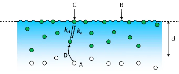
Consider a situation in which a single fluorescent species in solution interacts with binding sites on a surface through a simple, reversible bimolecular reaction (Figure 2.2). Fluorescent molecules in solution with average concentration A are in equilibrium with unoccupied, nonfluorescent surface binding sites of average density B, forming an average density of fluorescent, surface-bound complexes, C. The surface association and dissociation rate constants are denoted by ka and kd, respectively. The mechanism can be written as d a k C B A k (2.2)
where the equilibrium association constant describing the reaction is
AB C k k K d a
(2.3)
The total surface site density is denoted by S. Thus,
KA KAS C KA S B C B S 1
1 (2.4)
The total number of surface binding sites within the observed area is defined as N. In this case, KA KAN N KA N N N N S h
N B C B C
1 1 2
(2.5)
24
Figure 2.2: Reaction Mechanism. Fluorescent molecules in solution, A, reversibly bind to non-fluorescent surface sites, B, forming non-fluorescent complexes, C. The association and dissociation rates constants are ka and kd, respectively. The solution diffusion coefficient is D. The surface
binding sites and surface-bound complexes are not laterally mobile.
2.3.3 Fluorescence Fluctuation Autocorrelation Function
A general expression for G(τ) which accounts for fluorescence fluctuations
arising from diffusion through the evanescent field and from surface association and dissociation has previously been published (36). In this work, it is assumed that the surface binding sites and surface-associated complexes are not laterally mobile along the surface. Furthermore, it is assumed that the excitation intensity is low enough so that photo-physical processes do not contribute significantly to G(τ). The first assumption can be proven by using fluorescence recovery after photobleaching and the second can be shown by acquiring data as a function of the excitation intensity. The published general expression is rather complex (36). In the work described here, we consider the more simple form for G(τ) which is applicable when (1) the rates for diffusion in solution
through the observation volume are much faster than the rates associated with surface association and dissociation and (2) rebinding of previously dissociated fluorescent molecules within the small observed area is negligible. In this case,
) ( ) ( )
( Gs Ga
25
where the first term describes contributions to the autocorrelation function from surface binding kinetics and the second term describes contributions from diffusion of fluorescent molecules in solution but within the evanescent wave.
2.3.4 Magnitude of the Fluorescence Fluctuation Autocorrelation Function Because the observation volume is open with respect to coordinate z, fluctuations in the concentration of fluorescent molecules in solution obey Poisson statistics. However, because there is a finite number of surface binding sites in the observed area, fluctuations in the densities of surface-bound species obey binomial rather than Poisson statistics. These statements lead to the conclusion that (36)
2 2 ) ( ) 0 ( ) ( 2 ) 0 ( A C C B s A C A a N N N N N G N N N G
(2.7)
where the average number of unbound fluorescent molecules in the observed volume is
dA h
NA
2 (2.8)It is convenient to define a dimensionless quantity proportional to the solution concentration, X = KA. In this case, Eqs. 2.7 can be rewritten as
2 2 2 2 2 2 )] 1 ( [ ) 0 ( )] 1 ( [ 2 ) 1 ( ) 0 ( X d KS X h S K G X d KS X h X dK
Ga s
(2.9)
2.3.5 Time-Dependence of Ga(τ) As shown previously (9, 36),
26
where D is the diffusion coefficient of the fluorescent molecules in solution, Rz is the rate associated with diffusion in solution perpendicular to the surface and through the depth of the evanescent wave, and Rr is the rate associated with diffusion in solution parallel to the surface and through the extent of the observed area. Both factors in the first expression in Eq. 2.10 equal one when τ = 0 and monotonically decay to zero as τ → ∞. For a protein with a molecular weight of ≈ 100 kD, D ≈ 50 μm2
sec-1. Typically, d ≈ 0.1 μm, and h ≈ 0.5 μm, so that, for this value of D, Rz ≈ (0.2 ms)-1 and Rr ≈ (1.25 ms)-1. The minimum decay rate of Ga(τ) is Rz; Rr only speeds the decay.1
2.3.6 Time-Dependence of Gs(τ)
Given the assumptions that the rates for diffusion in solution through the observation volume are much faster than the rates associated with surface association and dissociation and that rebinding of previously dissociated fluorescent molecules within the small observed area is negligible, Gs(τ) has the form of an exponential decay (36, 37):
) 1 ( ) exp( ) 0 ( ) ( X k A k k G G d a d s
s
(2.11)
The first expression decays from one to zero with time. 2.4 Results
2.4.1 Measurement of K by Steady-State TIRFM
27
QdA A
F
dA KA KAS Q A F
neg pos
) (
] 1
[ ) (
(2.12)
where Fpos(A) is the fluorescence measured for surfaces containing binding sites, the first term in Fpos(A) arises from fluorescent ligands bound to surface sites, the second term in Fpos(A) arises from fluorescent molecules in solution but close enough to the surface to be excited by the evanescent wave, Fneg(A) is the fluorescence measured for surfaces not containing binding sites, and Q is a proportionality constant.
The difference between the fluorescence measured in the presence (S > 0) and absence (S = 0) of surface binding sites has the shape of a standard binding isotherm which can be curve-fit as a function of A to find the best value of K (and QS). The primary limitation of this type of measurement is that the surface site density in the positive samples must be high enough so that the first term in Eq. 2.12 is not overwhelmed by the second term. This feature is illustrated in Figure 2.3. As shown, higher binding site densities are required for lower values of K. If a general rule is set that the fluorescence measured in the presence of binding sites must be at least twice that measured in the absence of binding sites when A = K-1, then one finds that S ≥ 2d/K. Thus, when d = 0.1 μm, the approximate lower limit for S ranges from 12,000 molecules/μm2
28
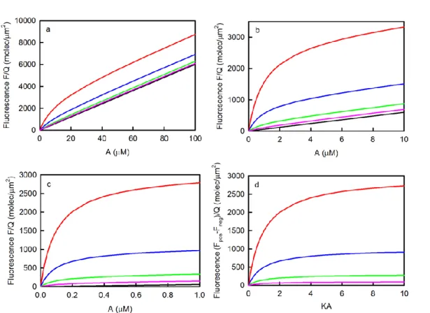
Figure 2.3: Measurement of K by Steady-State TIRFM. These plots show the values of Eq. 2.12 for d = 0.1 μm and K equal to (a) 105M-1, (b) 106M-1 or (c) 107M-1. The surface site densities S in units of molecules/μm2
are (red) 3000, (blue) 1000, (green) 300, (pink) 100 or (black) zero. The difference between the values shown in (a-c) with S > 0 and with S = 0 have the same shape when plotted as a function of the product of K and A and are shown in panel (d).
2.4.2 Criteria for TIR-FCS
As shown in the previous section, G(τ) is predicted to depend on a rather large
number of parameters, some of which are experimentally adjustable and some of which will be intrinsic to a given system of interest. Because so many parameters are present in the expression specifying the autocorrelation function and because all measured G(τ) will
29 and D (50 μm2
s-1), leaving four free parameters rather than seven. In addition, in many cases we have assumed that ka = 106 M-1s-1 as is common for processes at surfaces, thus fixing the value of kd given a value for K, leaving three free parameters: K, X, and S. Although these selections may not apply to a given system being considered for investigation, the procedure we outline below is readily amenable to generalization. Table 2.1: Parameters Governing the Behavior of G(τ)
Parameter Description
A average concentration of fluorescent molecules in solution
K (*) equilibrium association constant for fluorescent molecules and surface binding sites X(*) product of KandA
ka (***) kinetic association rate constant for fluorescent molecules and surface binding sites kd kinetic dissociation rate for fluorescent molecules and surface binding sites
S (*) total surface site density d (**) evanescent wave depth h (**) radius of observed area
D (**) solution diffusion coefficient of fluorescent molecules
Rz rate for diffusion in solution of fluorescent molecules through the evanescent wave Rr rate for diffusion in solution of fluorescent molecules through the observed area
There are three free (*), three fixed (**) and one partially fixed (***) parameters. The other four quantities depend on different subsets of these parameters as described in the text.
This work addresses combinations of the values of the three free parameters which will reasonably allow measurement by TIR-FCS of properties describing the thermodynamic and kinetic behavior of the mechanism shown in Figure 2.2. The criteria that we use are defined in Table 2.2: (A) G(τ) decays with reasonable rapidity so that data can be acquired in a reasonable amount of time. (B) Diffusion through the evanescent wave is fast enough so that Eqs. 2.6 and 2.11 are applicable (36); worth noting is that Rr only increases the decay rate of Ga(τ) over that determined by Rz.1
30
fluorescence fluctuation autocorrelation functions with magnitudes much lower than the minimum given in Table 2.2 are often measurable, in all but the simplest case (Eq. 2.11), Gs(τ) is not a single exponential (35) and higher values of Gs(0) are required to resolve,
for example, the rates and relative amplitudes associated with two exponentials. (D) The magnitude of Gs(τ) is high enough so that G(τ) is not dominated by Ga(τ). (E) Significant
rebinding to the surface within the observed area does not occur so that Eqs. 2.6 and 2.11 are applicable.
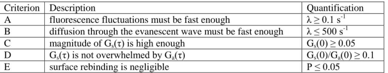
Table 2.2: Criteria
Criterion Description Quantification
A fluorescence fluctuations must be fast enough λ ≥ 0.1 s-1
B diffusion through the evanescent wave must be fast enough λ ≤ 500 s-1
C magnitude of Gs(τ) is high enough Gs(0) ≥ 0.05
D Gs(τ) is not overwhelmed by Ga(τ) Gs(0)/Ga(0) ≥ 0.1
E surface rebinding is negligible P ≤ 0.05
This table describes the criteria used to determine conditions for which TIR-FCS can measure thermodynamic and kinetic parameters describing the interaction of fluorescent molecules with surface binding sites given that the mechanism is a simple bimolecular reaction as defined in Eq. 2.2.
2.4.3 Experimental Conditions that Meet the Criteria
Criterion A requires that the fluorescence fluctuations be fast enough for G(τ) to be measurable with a good signal-to-noise ratio. We have quantified this criterion by specifying that Gs(τ) decays with a rate ≥ 0.1 s-1
. Referring to Eq. 2.11, one sees that the decay rate for Gs(τ) will always be ≥ kd. Thus, assuming that ka = 106 M-1s-1 (see above), K ≤ 107
M-1 (Eq. 2.3).
Criterion B requires that the decay rate of Gs(τ) be at least ten times slower than Rz (5000 s-1). To determine ka, it would be far above sufficient to obtain G(τ) for values of kaA = 4kd (λ = 5kd in Eq. 2.11). In this case, the decay rate of Gs(τ) for K = 107
31
would range from 0.1 to 0.5 s-1, meeting criterion B. The minimum value of 5kd is 500 s -1
, implying that (with ka = 106 M-1s-1) K ≥ 104 M-1.
Criteron C requires that Gs(0) ≥ 0.05. Although this condition might seem to be
too restrictive, it has been adopted primarily because we are ultimately interested in Gs(τ) that are more complex than Eq. 2.11 (see above). Gs(0) depends on three independent parameters (K, S and X) (Eq. 2.9), not including those that have been set at fixed values (h and d). Table 2.3 shows the conditions which conform to criterion C for different values of K, S and X. Worth noting first is that the partial derivative of Gs(0) with respect to X is negative, indicating that Gs(0) increases with decreasing X for set values of S and K. Second, the partial derivative of Gs(0) with respect to K is positive, indicating that Gs(0) increases with increasing K for set values of S and X. Third, the situation is a bit more complex when one considers the dependence of Gs(0) on S. In this case, each value of K and X has a value of S for which Gs(0) is maximized, found from the partial derivative of Gs(0) with respect to S. These values of S, denoted by Smax, are
K X d
Smax (1 )
(2.13)
and are shown in Table 2.3. By using Eq. 2.13 in Eq. 2.9, one finds that, when S = Smax,
) 1 ( 4 )] 0 (
[ max 2
X dX h K Gs (2.14)
32
The values of Xmax are given as upper limits in Table 2.3. Fourth, there are two values of S for which Gs(0) = 0.05 (criterion C), denoted as S1,2, which bracket the acceptable range of surface site densities. These values, found by setting Gs(0) in Eq. 2.9 equal to 0.05, are KX h X dKX h K X dX h K S 2 2 2 2 2 , 1 ) 1 ( 5 10 ) 1 ( 10
. (2.16)
S1 and S2 are real for X ≤ Xmax. When X=Xmax, the square root in Eq. 2.16 is zero and S1=S2=Smax. In some cases, the minimum value of S, S1, is < 1 molecule/μm2. Because h = 0.5 μm, the approximate size of the observed area is πh2
34
Criteron D requires that the ratio of Gs(0) and Ga(0) be ≥ 0.1, so that the long-time tail of Ga(τ) does not overlap too much with Gs(τ). This ratio (see Eqs. 2.9) is
2 ) 1 ( 2 ) 0 ( ) 0 ( X d KS G G a s (2.17)
and, as shown, increases with K and S; and decreases with X and d. However, when S = Smax, Gs(0)/Ga(0) = 2/(1 + X) and depends only on X (Figure 2.4b). In this case, because X is always less than or approximately equal to 0.64 (Table 2.3), the ratio ranges from ≈
2 at low X to 1.2, well above 0.1. In general, for a given value of K and X, an initial maximum value of Gs(0)/Ga(0) can be found with S = S2. As shown in Figure 2.4b, these maximum values of the ratio are all much greater than 0.1, so that in these cases criterion D is always satisfied. However, for a given value of K and X, the minimum value of the surface site density, according to criterion C, is for S = S1, and as shown in Figure 2.4b, the ratios Gs(0)/Ga(0) for S1 are not all greater than the allowed value of 0.1. This result sets a new minimum for the site density, denoted by S3, which is determined by setting the expression for the ratio in Eq. 2.17 equal to 0.1 and solving for the value of S. The values of S3 are
K X d S 20 ) 1 ( 2 3 (2.18)
35
Figure 2.4: Conditions Required for TIR-FCS. In all panels, the colors denote (red) K = 107 M-1; (blue) K = 3 x 10⁶ M-1; (green) K = 106 M-1; (pink) K = 3 x 10⁵ M-1;(cyan) K = 105 M-1; (dark red) K = 3 x 10⁴ M-1; and (dark green) K = 104 M-1. Panel (a) shows the values of [Gs(0)]max
calculated from Eq. 2.14 and as a function of X. In these plots, S = Smax (Eq. 2.13 and Table 2.3).
The black line depicts the cutoff values of X for which Gs(0) ≤ 0.05 and criterion C is not
satisfied. Panel (b) shows the values of Gs(0)/Ga(0) calculated from Eq. 2.17 and as a function of
X. Solid, colored lines are for S = S2 and dashed, colored lines are for S = S1. The solid black line
is for S = Smax and does not depend on K. The dashed black line shows the cutoff value below
which the ratio is unacceptable according to criterion D. Panel (c) shows P calculated by numerically integrating Eq. 2.19 with Eq. 2.20. The value of ka is taken to equal 10
6
M-1s-1 and the values of S are (solid) S2; (dash) Smax; and (dash-dot) the maximum of S1 and S3. The black
line depicts the cut-off value for which P ≥ 0.05 and criterion E is not satisfied.
36
molecule which dissociates from the origin at time zero has rebound at least once between positions r = 0 and r = h, and at time infinity, is
)] ( ) exp( [ )] 4 exp( 1 [ )] ( ) [exp( ) 4 exp( 4 2 2 0 2 2 0 2 0 0 t erfc t t Dt h dt t erfc t t Dt r Dt r dr d dt P h
(2.19)In Eqs. 2.19, the parameter η describes the propensity for surface rebinding and is defined
as ) 1 ( X D S ka (2.20)
Rebinding is more likely when the surface site density is higher, when the surface binding sites are less occupied, when the association kinetic rate constant is higher, and when the diffusion coefficient in solution is small. When h → ∞, the integral in Eq. 2.19
is (45)
1 )] ( ) exp( [ )] ( ) exp( [ ]
[ 2 2 0
0
t erfc t t erfc tt dt
P h (2.21)
A molecule which dissociates from an infinite plane always eventually rebinds somewhere on the surface. However, in the work described in this paper, h is small and the values of P are also (usually) small. Values of P as a function of X, with ka = 106 M -1
37 molecules/μm2
. The true maximum site densities are equal to the minima of S2 and S4 and are shown as upper limits in the S ranges in Table 2.3. [For the lowest K, Smax is greater than the upper limit and, when X=Xmax (0.00106), the upper limit is less than the lower limit, and therefore no values of S meet all five criteria. These results set a new upper limit for X (9.65x10⁻⁴).]
2.4.4 Measurement of K by TIR-FCS
A first question, given that criteria A-E are satisfied, is how one might go about measuring the equilibrium association constant K by using TIR-FCS rather than steady-state TIRFM. This type of measurement might be useful for a number of situations. One class of such situations includes in vivo cases in which the parameters cannot be precisely controlled or known (e.g., when one is interested in examining reversible association of fluorescent molecules in the cytosol with sites on the cytoplasmic face of adherent cells illuminated by evanescent excitation). Another class includes those in which one finds it not to be possible to make steady-state in vitro TIRFM measurements up to A ≈ 4/K (see above) because the required higher concentrations of fluorescent ligands with good purity are not obtainable within a reasonable amount of time and expense, or precipitate and/or oligomerize at high concentrations. Thus, we define below two methods in which K might be measured by using TIR-FCS.
First, it should be noted that measures of Fpos(A) and Fneg(A) (Eq. 2.12) will be a natural consequence of acquiring TIR-FCS data. No extraneous steady-state TIRFM data acquisition is required. Then, from the two measured quantities, one can calculate
KA KA d KS A F A F A F neg neg pos 1 1 1 ) ( ) ( ) ( (2.22)
38
d KS
(2.23)
The wide range of ρ values (0.05 to 550) for different values of K and X are shown in
Table 2.3. Curve-fitting the measured values of Eq. 2.22 to the form on the right side, as a function of A, will give a best-fit value for ρ and, if high enough A values are accessible, also for K. If one chooses to assume an approximate value for d (1), then an approximate value for S can be found from ρ, K and d. Predicted data are illustrated in
Figure 2.5a. As shown, this strategy for measuring K is more likely to be successful for higher K values. Because the accessible values of X are capped at very low values for smaller K (Table 2.3), in these cases Eq. 2.22 is approximately constant and equal to ρ. Thus, low K values are predicted to be measurable by this method only if the values of S and d are independently calibrated.
Figure 2.5: Measurement of K by using TIR-FCS. In both panels, the colors denote (red) K = 107 M-1, (blue) K = 3 x 10⁶ M-1, (green) K = 106 M-1, and (pink) K = 3 x 10⁵ M-1; surface site densities are (red) 1, (blue) 3.33, (green) 10, and (pink) 33.3 molecules/μm2; and ρ = 0.166.
Panel (a) shows the values of [Fpos(A)-Fneg(A)]/Fneg(A) calculated from Eq. 2.22. The intercepts
equal ρ. The initial slopes equal –ρK; their magnitudes increase with K. These slopes are indicative of the ability of the proposed strategy to measure K. Panel (b) shows the values of [Gneg(0)-Gpos(0)]/[Gneg(0)] calculated from Eq. 2.25. The intercepts equal [ρ/(1+ρ)]
2
. The initial slopes are 2Kρ/(1+ρ)3
39
Because measuring equilibrium association constants by using only values of A that are less than K-1 is vulnerable to potential artifacts, it is desirable to confirm the measured K value by using the information contained in the magnitudes of the acquired G(τ). There are two directly measurable quantities, G(0) in the presence and absence of
surface binding sites, denoted as Gpos(0) and Gneg(0), respectively. Referring to Eqs. 2.6 and 2.9, one finds that
dA h G KA d KS A h KA d KS G neg pos 2 2 2 2 2 1 ) 0 ( )] 1 ( [ 2 ) 1 ( 2 ) 0 ( (2.24)
To accurately measure these quantities, it may be necessary to account for photophysical effects that can occur at high excitation intensities and low time lags τ (27, 28). This
correction is necessary only if the excitation intensity is high enough so that the measured G(τ) are dependent on it. In addition, the G(0) values must be extrapolated from G(τ) at low τ because when τ = 0 the autocorrelation functions contain contributions from shot
noise. In analogy to Eq. 2.22, the following function can be defined:
2 2 ) 1 ( ) 2 ( )] 1 ( [ ] 2 [ ) 0 ( )] 0 ( ) 0 ( [ KA KA KA d KS dKA KS KS G G G neg pos neg (2.25)