Analysis of the Load Flow Problem in Power System Planning Studies

http://dx.doi.org/10.4236/epe.2015.710048

Analysis of the Load Flow Problem in Power

System Planning Studies

Olukayode A. Afolabi, Warsame H. Ali, Penrose Cofie, John Fuller, Pamela Obiomon,

Emmanuel S. Kolawole

Department of Electrical and Computer Engineering, Prairie View A&M University, Prairie View, USA Email: oafolabi@student.pvamu.edu, whali@pvamu.edu, pscofie@pvamu.edu, jhfuller@pvamu.edu,

pobiomon@pvamu.edu, ekolawole@student.pvamu.edu

Received 10 August 2015; accepted 27 September 2015; published 30 September 2015

Copyright © 2015 by authors and Scientific Research Publishing Inc.

This work is licensed under the Creative Commons Attribution International License (CC BY).

http://creativecommons.org/licenses/by/4.0/

Abstract

Load flow is an important tool used by power engineers for planning, to determine the best opera-tion for a power system and exchange of power between utility companies. In order to have an ef-ficient operating power system, it is necessary to determine which method is suitable and efef-ficient for the system’s load flow analysis. A power flow analysis method may take a long time and there-fore prevent achieving an accurate result to a power flow solution because of continuous changes in power demand and generations. This paper presents analysis of the load flow problem in power system planning studies. The numerical methods: Gauss-Seidel, Newton-Raphson and Fast De-coupled methods were compared for a power flow analysis solution. Simulation is carried out us-ing Matlab for test cases of IEEE 9-Bus, IEEE 30-Bus and IEEE 57-Bus system. The simulation re-sults were compared for number of iteration, computational time, tolerance value and conver-gence. The compared results show that Newton-Raphson is the most reliable method because it has the least number of iteration and converges faster.

Keywords

Load Flow, Bus, Gauss-Seidel, Newton-Raphson, Fast Decoupled, Voltage Magnitude, Voltage Angle, Active Power, Reactive Power, Iteration, Convergence

1. Introduction

flow studies provide a systematic mathematical approach to determine the various bus voltages, phase angles, active and reactive power flows through different branches, generators, transformer settings and load under steady state conditions. The power system is modeled by an electric circuit which consists of generators, trans-mission network and distribution network [1].

The main information obtained from the load flow or power flow analysis comprises magnitudes and phase angles of load bus voltages, reactive powers and voltage phase angles at generator buses, real and reactive power flows on transmission lines together with power at the reference bus; other variables being specified [2] [3]. The resulting equations in terms of power, known as the power flow equations become non-linear and must be solved by iterative techniques using numerical methods. Numerical methods are techniques by which mathe-matical problems are formulated so that they can be solved with arithmetic operations and they usually provide only approximate solution.

For the past three decades, various numerical analysis methods have been applied in solving load flow analy-sis problems. The most commonly used iterative methods are the Gauss-Seidel, the Newton-Raphson and Fast Decoupled method [4]. Also with the industrial developments in the society, the power system kept increasing and the dimension of load flow equation also kept increasing to several thousands. With such increases, any numerical mathematical method cannot converge to a correct solution. Thus power engineers have to seek more reliable methods. The problem that faces power industry is how to determine which method is most suitable for a power system analysis. In power flow analysis, a high degree accuracy and a faster solution time are required to determine which method is best to use.

Hand calculations are suitable for the estimation of the operating characteristics of a few individual circuits, but accurate calculations of load flows or short circuits analysis’ would be impractical without the use of com-puter programs. The use of digital comcom-puters to calculate load flow started from mid 1950s. There have been different methods used for load flow calculation. The development of these methods is mainly led by the basic requirement of load flow calculation such as convergence properties, computing efficiency, memory require-ment, convenience and flexibility of the implementation [5]-[9]. With the availability of fast and large size digi-tal computers, all kinds of power system studies, including load flow, can now be carried out conveniently [10]. The numerical method provides an approach to find solution with the use of computer, therefore there is need to determine which of the numerical method is faster and more reliable in order to have best result for load flow analysis.

This paper compares numerical methods: Gauss-Seidel, Newton-Raphson and Fast Decoupled methods use for load flow analysis; for test cases of IEEE 9-Bus, IEEE 30-Bus and IEEE 57-Bus system to determine which of the method is best for power system planning studies.

2. Bus Classification

A bus is a point or node in which one or many transmission lines, loads and generators are connected. In a pow-er system study, evpow-ery bus is associated with 4 quantities, such as magnitude of voltage (|V|), phase angle of voltage (δ), active power (P) and reactive power (Q) [2] [3] [11] [12]. Two of these bus quantities are specified and the remaining two are required to be determined through the solution of equation [13]. The buses are classi-fied depending on the two known quantities that have been speciclassi-fied. Buses are divided into three categories as shown inTable 1.

2.1. Slack Bus

This is used as a reference bus in order to meet the power balance condition. Slack bus is usually a generating unit that can be adjusted to take up whatever is needed to ensure power balanced [12]. The effective generator at this bus supplies the losses to the network, this is necessary because the magnitude of the losses will not be known until the calculation of the current is complete. Slack bus is usually identified as bus 1. The known varia-ble on this bus is |V| and δ and the unknown is P and Q.

2.2. Generator (PV) Bus

[image:3.595.146.485.95.195.2]

Table 1. Bus classification.

No. Type of Bus

Variables

P Q |V| δ

1 Slack Bus Unknown Unknown Known Known

2 Generator Bus (PV) Known Unknown Known Unknown

3 Load Bus (PQ) Known Known Unknown Unknown

of the generator. Often, limits are given to the values of the reactive power depending upon the characteristics of individual machine. The known variable in this bus is P and |V| and the unknown is Q and δ [8] [12].

2.3. Load (PQ) Bus

This is a non-generator bus which can be obtained from historical data records, measurement or forecast. The real and reactive power supply to a power system are defined to be positive, while the power consumed in a power system are defined to be negative. The consumer power is met at this bus. The known variable for this bus is P and Q and the unknown variable is |V| and δ[8] [12].

3. Power Flow Analysis Methods

The numerical analysis involving the solution of algebraic simultaneous equations forms the basis for solution of the performance equations in computer aided electrical power system analyses e.g. for load flow analysis [4]. The first step in performing load flow analysis is to form the Y-bus admittance using the transmission line and transformer input data. The nodal equation for a power system network using Y bus can be written as follows:

Bus

I =Y V (1) The nodal equation can be written in a generalized form for an n bus system.

1 for 1, 2, 3, n

i j ij j

I =

∑

₌Y V i= n (2) The complex power delivered to bus i is

i i i i

P+ jQ =V I∗ (3)

i i

i i

P jQ

I

V∗

−

= (4)

Substituting for Ii in terms of Pi&Qi, the equation gives

1 1

n n

i i

i j ij j ij j

i

P jQ

V y y V j i

V∗ = =

− _{= − ≠}

∑

∑

(5)

The above equation uses iterative techniques to solve load flow problems. Hence, it is necessary to review the general forms of the various solution methods; Gauss-Seidel, Newton Raphson and Fast decoupled load flow.

3.1. Gauss-Seidel Method

This method is developed based on the Gauss method. It is an iterative method used for solving set of nonlinear algebraic equations [14]. The method makes use of an initial guess for value of voltage, to obtain a calculated value of a particular variable. The initial guess value is replaced by a calculated value. The process is then re-peated until the iteration solution converges. The convergence is quite sensitive to the starting values assumed. But this method suffers from poor convergence characteristics [15].

( ) ( ) 1 sch sch k i i ij j k i i ij P jQ y V V

V j i

y

∗ +

− ₊

=

∑

≠

∑

(6) Using Kirchhoff current law, it is assumed that the current injected into bus i is positive, then the real and the reactive powers supply into the buses, such as generator buses, P_isch and Q_isch have a positive value. The real and the reactive powers flowing away from the buses, such as load buses P_isch and Q_isch have a negative val-ues. Pi and Qi are solved from Equation (5) which gives

( 1) ( )

{

( )

}

0

Real n n

k k k

i i i ij ji i

P + = _V∗

∑

₌ y −

∑

V _ j≠i (7)

( 1) ( )

{

( )

}

1

Imaginary n n

k k k

i i j ij ji i

Q + = _V∗

∑

₌ y −

∑

V _ j≠i (8)

The power flow equation is usually expressed in terms of the bus admittance matrix, using the diagonal elements of the bus admittance and the non-diagonal elements of the matrix, then the Equation (6) becomes,

( ) ( ) *( ) 1 sch sch k i i ij j k k i I ii P jQ Y V V V Y + − ₋

=

∑

(9)

and

( 1) ( )

{

( ) ( )

}

1, 1

Real n

k k k k

i i i ii i j ij j

P + = _V∗ V∗ Y +

∑

_{= =} y V _ j≠i (10)

( 1) ( )

{

( ) ( )

}

1, 1

Imaginary n

k k k k

i i i ii i j ij j

P + = _V∗ V∗ Y +

∑

_{= =} y V _ j≠i (11)

The admittance to the ground of line charging susceptance and other fixed admittance to ground are included into the diagonal element of the matrix.

3.2. Newton-Raphson Method

This method was named after Isaac Newton and Joseph Raphson. The origin and formulation of Newton-Ra- phson method was dated back to late 1960s [7]. It is an iterative method which approximates a set of non-linear simultaneous equations to a set of linear simultaneous equations using Taylor’s series expansion and the terms are limited to the first approximation. It is the most iterative method used for the load flow because its conver-gence characteristics are relatively more powerful compared to other alternative processes and the reliability of Newton-Raphson approach is comparatively good since it can solve cases that lead to divergence with other popular processes [15]. If the assumed value is near the solution, then the result is obtained very quickly, but if the assumed value is farther away from the solution then the method may take longer to converge [12]. This is another iterative load flow method which is widely used for solving nonlinear equation.

The admittance matrix is used to write equations for currents entering a power system. Equation (2) is expressed in a polar form, in which j includes bus i

1 n

i j ij i ij j

I =

∑

₌ Y V <θ +δ (12)

The real and reactive power at bus i is

i i i i

P−jQ =V I∗ (13) Substituting for Ii in Equation (12) from Equation (13)

1

i i i i ij

n

j j ij j

(

)

1 cos

n

i j i j ij ij i j

P=

∑

₌ V V Y θ − +δ δ (15)

(

)

1 sin

n

i j i j ij ij i j

Q =

∑

₌ V V Y θ − +δ δ (16)

The above Equation (15) and (16) constitute a set of non-linear algebraic equations in terms of |V| in per unit and δ in radians. Equation (15) and (16) are expanded in Taylor’s series about the initial estimate and neglecting all higher order terms, the following set of linear equations are obtained.

( ) ( ) ( ) ( ) ( ) ( ) ( ) ( ) ( ) ( ) ( ) ( ) ( ) ( ) ( ) ( ) ( ) ( ) ( ) ( ) 2 2 2 2 2 2 2

2 2 2 2

2

2 2 2

2

2 2

k k k k

k

k k k k

n

n n

n n

n n n

k n

K K K K K

k n

K K K K

n n n n

n n

n n

P P P P

P

P P P P

P

Q Q Q Q Q

Q Q V V Q Q V V V V V Q V δ δ δ δ δ δ δ δ ∂ ∂ ∂ ∂ ∆ ∂ ∂ ∂ ∂    _{∂ ∂ ∂ ∂}                    _{∂ ∂ ∂ ∂}    _{ = }        ∂ ∂ ∂ ∂              ∂ ∂ ∂ ∂  ∆ ∆ ∂ ∂ ∂ ∂ ∆ ∂ ∂ ∂ ∂                        ( ) ( ) ( ) ( ) 2 2 k k n K k n P P Q Q                        ∆ ∆ ∆     ∆    

In the above equation, the element of the slack bus variable voltage magnitude and angle are omitted because they are already known. The element of the Jacobian matrix are obtained after partial derivatives of Equations (15) and (16) are expressed which gives linearized relationship between small changes in voltage magnitude and voltage angle. The equation can be written in matrix form as:

1 3 2 4 J J P V J J Q δ ∆ ∆     ₌     _∆  _∆

      (17)

J1, J2, J3, J4 are the elements of the Jacobian matrix.

The difference between the schedule and calculated values known as power residuals for the terms ∆P_i( )k and ∆Q_i( )k is represented as:

( )k sch ( )k

i i i

P P P

∆ = − (18)

( )k sch ( )k

i i i

Q Q Q

∆ = − (19)

The new estimates for bus voltage are

(k 1) ( )k ( )k

i i

δ

+ ₌

δ

_{+ ∆}

δ

(20)

(k1) ( )k ( )k

i i

V + =V + ∆V (21)

3.3. Fast Decoupled Method

This method is a modification of Newton-Raphson, which takes the advantage of the weak coupling between P−δ and Q−V due to the high X:R ratios. The Jacobian matrix of Equation (17) is reduced to half by ig-noring the element of J2 and J3. Equation (17) is simplified as:

1 4 0 0 J P V J Q δ ∆ ∆      =_{  } _∆  _∆

      (22)

Expanding Equation (22) gives two separate matrixes,

1

P

P J δ δ

δ ∂   ∆ = ∆ =_{ }∆

∂

  (23)

4

P

Q J V V

V

 _∂  ∆ = ∆ =_{ }∆

∂  

  (24)

i P B V δ ∆ _{= − ∆′} (25) i Q B V V ∆ _{= − ∆′′} (26)

B' and B'' are the imaginary parts of the bus admittance. It is better to ignore all shunt connected elements, as to make the formation of J1 and J4 simple. This will allow for only one single matrix than performing repeated in-version .The successive and voltage magnitude and phase angle changes are

[ ]

1 P

B V

δ _′− ∆

∆ = − (27)

[ ]

1 Q

V B

V

− ∆

′′

∆ = − (28)

4. Simulation Results

[image:6.595.245.525.128.324.2]

The simulation for Gauss-Seidel, Newton-Raphson and Fast Decouple is carried out using Matlab for test cases of IEEE 9. The base mva, selected valve for iteration (tolerance), and maximum numbers of iterations is speci-fied.Figure 1 show IEEE 9-Bus System one line diagram, [12]. The simulation results are shown inFigure 2, Figure 3andFigure 4 for Gauss-Seidel, Newton-Raphson and Fast Decouple respectively.

IEEE 9 bus system represented in Table 2 consist of Bus 1 which act as a slack bus. It consist of 8 load buses, which are bus connected to load and 2 generator buses which are connected to generator. Bus 5 and 8 act as both load and generator bus because they are connected to generator and load.

[image:6.595.226.403.568.705.2]

Figure 2. Show simulation result for IEEE 9 bus system using gauss-seidel.

Figure 3. Show the simulation result for Newton-Raphson method on a 9 bus network system.

IEEE 9-bus system consist of eleven line data as represented inTable 3, which shows the values for resis-tance, reactance and half susceptance in per unit for the transmission line connected together. It also shows the tap setting values for transformers and the position of the transformers on the transmission line. The information is used to form the admittance bus matrix.

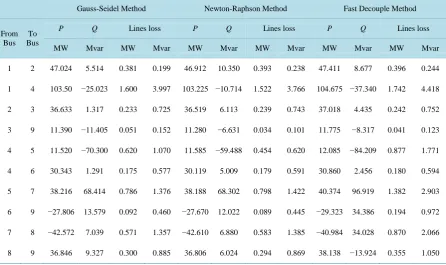
[image:8.595.146.483.219.706.2]

Table 4represents the line flow and line losses for each of the IEEE 9 bus system. The line losses are com-pared for the three numerical methods; Gauss-Seidel, the Newton-Raphson and Fast Decoupled method. Fast Decoupled method have the highest total losses of 6.279 MW, 14.893 Mvar, followed by Gauss-Seidel with to-tal losses of 4.809 MW, 10.798 Mvar and Newton Raphson method with the least losses of 4.585 MW and 10.789 Mvar.

Table 2. Load data of IEEE 9 bus system.

LOAD DATA

Bus Type of Bus

Voltage Load Generation

V (P.U) δ (θ) P (MW) Q (Mvar) P (MW) Q (Mvar)

1 Slack 1.0300 0 0 0

2 PQ 1.0000 0 10 5

3 PQ 1.0000 0 25 15

4 PQ 1.0000 0 60 40

5 PQ 1.0600 0 10 5 80

6 PV 1.0000 0 100 80

7 PQ 1.0000 0 80 60

8 PV 1.0100 0 40 20 120

[image:8.595.143.484.471.717.2]

9 PQ 1.0000 0 20 10

Table 3. Line data of IEEE 9 bus system.

LINE DATA

Bus No. Bus No. R, PU X, PU 1/2 B, PU Transformer Tap

1 2 0.0180 0.0540 0.0045 1

1 4 0.0150 0.0450 0.0038 1

2 3 0.0180 0.0560 0 1

3 9 0.0200 0.0600 0 1

4 5 0.0130 0.0360 0.0030 1

4 6 0.0200 0.0660 0 1

5 6 0.0600 0.030 0.0028 1

5 7 0.0140 0.0360 0.0030 1

6 9 0.0100 0.0500 0 1

7 8 0.0320 0.0760 0 1

[image:9.595.90.537.103.368.2]

Table 4. Line flow and losses comparing for IEEE 9 bus system.

Gauss-Seidel Method Newton-Raphson Method Fast Decouple Method

From Bus

To Bus

P Q Lines loss P Q Lines loss P Q Lines loss

MW Mvar MW Mvar MW Mvar MW Mvar MW Mvar MW Mvar

1 2 47.024 5.514 0.381 0.199 46.912 10.350 0.393 0.238 47.411 8.677 0.396 0.244

1 4 103.50 −25.023 1.600 3.997 103.225 −10.714 1.522 3.766 104.675 −37.340 1.742 4.418

2 3 36.633 1.317 0.233 0.725 36.519 6.113 0.239 0.743 37.018 4.435 0.242 0.752

3 9 11.390 −11.405 0.051 0.152 11.280 −6.631 0.034 0.101 11.775 −8.317 0.041 0.123

4 5 11.520 −70.300 0.620 1.070 11.585 −59.488 0.454 0.620 12.085 −84.209 0.877 1.771

4 6 30.343 1.291 0.175 0.577 30.119 5.009 0.179 0.591 30.860 2.456 0.180 0.594

5 7 38.216 68.414 0.786 1.376 38.188 68.302 0.798 1.422 40.374 96.919 1.382 2.903

6 9 −27.806 13.579 0.092 0.460 −27.670 12.022 0.089 0.445 −29.323 34.386 0.194 0.972

7 8 −42.572 7.039 0.571 1.357 −42.610 6.880 0.583 1.385 −40.984 34.028 0.870 2.066

8 9 36.846 9.327 0.300 0.885 36.806 6.024 0.294 0.869 38.138 −13.924 0.355 1.050

5. Discussion

5.1. Tolerance

The selected tolerance iteration value used for the simulation is shown inTable 5. This is used to determine how accurate a solution will be. Thus, using a high tolerance value for a simulation increases the accuracy of the so-lution whereas when a low tolerance value is used, it reduces the accuracy of the soso-lution and number of itera-tions. The selected tolerance value used for the simulation is 0.001 and 0.1 except for the IEEE 57 bus system solution for fast decouple, which does converge with 0.001. The only selected tolerance value used for IEEE 57 bus system is the 0.1.

5.2. Iteration Number

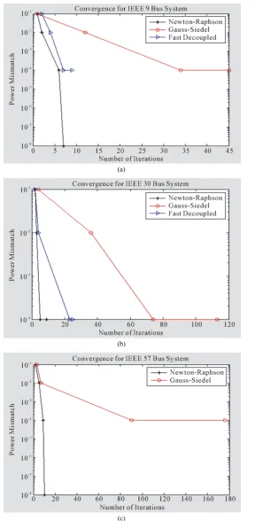
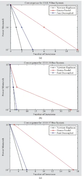
Table 6andTable 7 show the number of iterations for the power flow solution using selected iteration value of 0.001 and 0.1 respectively to converge for the three load flow methods. Gauss-Seidel has the highest number of iterations before it converges. The number of iteration increases as the number of buses in the system increases. In the 9 bus system and 30 bus system, Newton-Raphson has the least number of iteration to converge. For the 57 bus system using fast decouple, the load flow solution did not converge using 0.001. Then another selected value of 0.1 was chosen for the iteration.

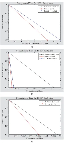
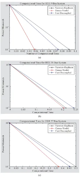
5.3. Computing Time

(a)

(b)

(c)

[image:10.595.177.454.81.684.2]

(a)

(b)

(c)

[image:11.595.177.454.82.687.2]

Table 5. Comparison of tolerance value.

Test System Gauss-Seidel Newton-Raphson Fast Decouple

IEEE 9 Bus 0.001/0.1 0.001/0.1 0.001/0.1

IEEE30 Bus 0.001/0.1 0.001/0.1 0.001/0.1

IEEE57 Bus 0.001/0.1 0.001/0.1 0.1

Table 6. Comparison of iteration number using selected iteration value of 0.001.

Test System Gauss-Seidel Newton-Raphson Fast Decouple

IEEE 9 Bus 45 7 9

IEEE 30 Bus 113 9 25

IEEE 57 Bus 176 10

Table 7. Comparison of iteration number using selected iteration value of 0.1.

Test System Gauss-Seidel Newton-Raphson Fast Decouple

IEEE 9 Bus 12 2 4

IEEE 30 Bus 36 4 3

[image:12.595.147.486.414.496.2]

IEEE 57 Bus 17 5 6

Table 8. Comparison of computing time using selected value of 0.001.

Test System Gauss-Seidel Newton-Raphson Fast Decouple

IEEE 9 Bus 0.003 0.004 0.004

IEEE 30 Bus 0.008 0.103 0.012

[image:12.595.146.483.522.599.2]

IEEE 57 Bus 0.008 0.013

Table 9. Comparison of computing time using selected iteration value of 0.1.

Test System Gauss-Seidel Newton-Raphson Fast Decouple

IEEE 9 Bus 0.038 0.091 0.074

IEEE 30 Bus 0.205 0.213 0.243

IEEE 57 Bus 0.367 0.500 0.455

5.4. Convergence

(a)

(b)

(c)

[image:13.595.175.464.81.671.2]

(a)

(b)

(c)

[image:14.595.179.456.82.671.2]

6. Conclusions

All the simulations were carried out using Mathlab and implemented for IEEE 9-bus, IEEE 30-bus and IEEE 57-bus test cases for Gauss-Seidel, Newton-Raphson and Fast Decouple. In the load flow analysis methods si-mulated, the tolerance values used for simulation are 0.001 and 0.1 for all the simulation carried out except for the IEEE 57-bus using the fast decouple method, which did not converge with the tolerance values. This ex-plains why the Fast Decouple method is not as accurate as Newton-Raphson method because a lower tolerance value of 0.1 was used to carry out the simulation for the IEEE 57-bus Fast Decouple Method.

The time for iteration in Gauss-Seidel is the longest compared to the other two methods, Newton-Raphson and Fast Decouple. The time for iterations in Gauss-Seidel increases as the number of buses increases. The Gauss-Seidel method increases in arithmetic progression, Newton-Raphson increases in quadratic progression while the fast decouple increases in geometric progression. This explains why it takes longer time for Gauss- Seidel to converge. The computational time for Gauss-Seidel is low compared to the other two methods; New-ton-Raphson and fast decouple. NewNew-ton-Raphson have more computational time due to the complexity of the Jacobian matrix for each iteration but still converges fast enough because less number of iterations are carried out and required.

The results of this paper suggest that the planning of a power system can be carried out by using Gauss-Seidel method for a small system with less computational complexity due to the good computational characteristics it exhibited. The effective and most reliable amongst the three load flow methods is the Newton-Raphson method because it converges fast and is more accurate.

References

[1] Mageshvaran, R., Raglend, I.J., Yuvaraj, V., Rizwankhan, P.G., Vijayakumar, T. and Sudheera (2008) Implementation of Non-Traditional Optimization Techniques (PSO, CPSO, HDE) for the Optimal Load Flow Solution. TENCON2008-

2008 IEEE Region 10 Conference, 19-21 November 2008.

[2] Elgerd, O.L. (2012) Electric Energy Systems Theory: An Introduction. 2nd Edition, Mc-Graw-Hill. [3] Kothari, I.J. and Nagrath, D.P. (2007) Modern Power System Analysis. 3rd Edition, New York.

[4] Keyhani, A., Abur, A. and Hao, S. (1989) Evaluation of Power Flow Techniques for Personal Computers. IEEE Trans- actions on Power Systems, 4, 817-826.

[5] Hale, H.W. and Goodrich, R.W. (1959) Digital Computation or Power Flow—Some New Aspects. Power Apparatus and Systems, Part III. Transactions of the American Institute of Electrical Engineers, 78, 919-923.

[6] Sato, N. and Tinney, W.F. (1963) Techniques for Exploiting the Sparsity or the Network Admittance Matrix. IEEE Transactions on Power Apparatus and Systems, 82, 944-950.

[7] Aroop, B., Satyajit, B. and Sanjib, H. (2014) Power Flow Analysis on IEEE 57 bus System Using Mathlab. Interna-tional Journal of Engineering Research & Technology (IJERT), 3.

[8] Milano, F. (2009) Continuous Newton’s Method for Power Flow Analysis. IEEE Transactions on Power Systems, 24, 50-57.

[9] Grainger, J.J. and Stevenson, W.D. (1994) Power System Analysis. McGraw-Hill, New York.

[10] Tinney, W.F. and Hart, C.E. (1967) Power Flow Solution by Newton’s Method. IEEE Transactions on Power Appa-ratus and Systems, PAS-86, 1449-1460.

[11] Bhakti, N. and Rajani, N. (2014) Steady State Analysis of IEEE-6 Bus System Using PSAT Power Tool Box. Interna-tional Journal of Engineering Science and Innovation Technology (IJESIT), 3.

[12] Hadi, S. (2010) Power System Analysis. 3rd Edition, PSA Publishing, North York. [13] Kabisama, H.W. Electrical Power Engineering. McGraw-Hill, New York.

[14] Gilbert, G.M., Bouchard, D.E. and Chikhani, A.Y. (1998) A Comparison of Load Flow Analysis Using Dist Flow, Gauss-Seidel, and Optimal Load Flow Algorithms. Proceedings of theIEEE Canadian Conference on Electrical and Computer Engineering, Waterloo, Ontario, 24-28 May 1998, 850-853.

[15] Glover, J.D. and Sarma, M.S. (2002) Power System Analysis and Design. 3rd Edition, Brooks/Cole, Pacific Grove. [16] Stott, B. and Alsac, O. (1974) Fast Decoupled Load Flow. IEEE Transactions on Power Apparatus and Systems,

PAS-93, 859-869.

[17] Stott, B. (1974) Review of Load-Flow Calculation Methods. Proceedings of the IEEE, 62, 916-929.