http://dx.doi.org/10.4236/ajcm.2015.53032
Nonlinear Waves in Solid Continua with
Finite Deformation
K. S. Surana1, J. Knight1, J. N. Reddy2
1Department of Mechanical Engineering, University of Kansas, Lawrence, KS, USA
2Department of Mechanical Engineering, Texas A & M University, College Station, TX, USA Email: [email protected], [email protected], [email protected]
Received 28 July 2015; accepted 7 September 2015; published 11 September 2015 Copyright © 2015 by authors and Scientific Research Publishing Inc.
This work is licensed under the Creative Commons Attribution International License (CC BY). http://creativecommons.org/licenses/by/4.0/
Abstract
This work considers initiation of nonlinear waves, their propagation, reflection, and their interac-tions in thermoelastic solids and thermoviscoelastic solids with and without memory. The con-servation and balance laws constituting the mathematical models as well as the constitutive theo-ries are derived for finite deformation and finite strain using second Piola-Kirchoff stress tensor and Green’s strain tensor and their material derivatives [1]. Fourier heat conduction law with constant conductivity is used as the constitutive theory for heat vector. Numerical studies are performed using space-time variationally consistent finite element formulations derived using space-time residual functionals and the non-linear equations resulting from the first variation of the residual functional are solved using Newton’s Linear Method with line search. Space-time local approximations are considered in higher order scalar product spaces that permit desired order of global differentiability in space and time. Computed results for non-linear wave propagation, ref-lection, and interaction are compared with linear wave propagation to demonstrate significant differences between the two, the importance of the nonlinear wave propagation over linear wave propagation as well as to illustrate the meritorious features of the mathematical models and the space-time variationally consistent space-time finite element process with time marching in ob-taining the numerical solutions of the evolutions.
Keywords
Linear and Nonlinear Waves, Second Piola-Kirchoff Stress, Green's Strain, Constitutive Theories, Dissipation, Memory, Rheology, Finite Strain
1. Literature Review, Outline, and Significance
deformation and finite strain is an area of significant interest due to the introduction of polymeric solids and their abundant use in industrial applications. Polymers can undergo finite deformation, finite strain, have a dis-sipation mechanism, and exhibit rheological behavior. Thus, the deformation physics in such materials is quite complex. Development of mathematical models for finite deformation and finite strain for solid continua in La-grangian description using conservation and balance laws resulting in initial value problems (IVP) and time ac-curate numerical simulations of the evolution described by the IVPs is the main objective of this research.
A review of the published works related to the research presented here is given in the following. In the pub-lished works cited and discussed here we address four basic questions: 1) what is the source of nonlinearity, 2) type of material considered (elastic, viscoelastic, etc.), 3) constitutive theories, 4) methodology or approach used to obtain numerical solution of the resulting mathematical model. In reference [2] conservation and balance laws are considered and some aspects of the constitutive theories are also discussed with the main objective of ob-taining simplified mathematical models with various assumptions that would permit theoretical or semianalyti-cal solutions. Many specialized forms of the 1D and 2D wave equations and their possible solutions are dis-cussed. Reference [3] considers solids under high-pressure shock compression. This book presents many aspects of mechanics, physics, and chemistry in such deformation. Plasticity or irreversible deformation processes are a central point of focus in this reference. The material in the book is largely devoted to experiments, design of ex-periments, and analysis of experimental data. Experimentally focused work on “nonlinear phenomena in the propagation of elastic waves in solids” is also presented in reference [4]. The authors consider Green’s strain and many applications to different and unique materials. Precise mathematical models used, the constitutive theories considered and their derivations are not given. In reference [5], the authors consider a one degree of freedom oscillator subjected to an external force and a restoring viscoelastic force with memory based on a phenomenological approach. Such models are not valid in the thermodynamic sense and their extension to R2 and R3 is not possible [1]. Finite amplitude waves in isotropic elastic plates are considered by Lima and Hamil-ton [6]. A perturbation technique with semianalytical solution is used to obtain the solutions of the governing equation of equilibrium in Lagrangian description. Periodic harmonic solutions are presented. In reference [7], thermoelastic small-amplitude wave propagation in nonlinear elastic media is considered. Helmholtz free energy density is expressed as a nonlinear function of the principal stretches and is used to derive the constitutive equa-tion for stress. For thermoelastic material based on reference [1], this approach of deriving constitutive theory is unfounded. This approach is applied to layered structures. Lima and Hamilton [8] presented a study of finite amplitude waves in isotropic elastic waveguides with arbitrary cross-sectional area using perturbation and modal analysis techniques to obtain the solutions of nonlinear equations of motion for harmonic motion. The second Piola-Kirchoff stress tensor is expressed as a quadratic function of the Green’s strain tensor using a special form given in references [9] [10]. A study of nonlinear deformation waves in solids and dispersion due to microstruc-tures using Mindlin type model is considered in reference [11]. Finite volume method is used to study tion and interaction of one-dimensional waves. Nonlinear transient thermal stresses and elastic wave propaga-tion studies in thick temperature-gradient dependent FGM cylinder using a second-order point-collocapropaga-tion me-thod are presented in reference [12]. In reference [13], numerical simulations of linear and nonlinear waves in hypoelastic solids are presented using conservation element and solution element method (CESE). These inves-tigations are hypothetical as the constitutive theories for hypoelastic solids are hypothetical since these constitu-tive theories cannot describe the constitution of solids. Numerical simulations of nonlinear elastic wave propa-gation in piecewise homogeneous media are considered in reference [14]. Wave reflection, transmission, and interaction of waves are not clearly demonstrated primarily due to complexity of the properties of the domain. Vibrations and wave propagation in thick FGM cylinders with temperature dependent material properties are investigated in reference [15]. A nodal discontinuous Galerkin finite element method is considered for nonlinear elastic wave propagation in reference [16]. Nonlinear transient stress wave propagation in thick FGM cylinder using a unified generalized thermoelasticity theory is considered in reference [17]. Nonlinear constitutive model for axisymmetric bending of annular graphene-like nanoplates with gradient elasticity enhancement effects is considered in reference [18]. In reference [19], nonlinear semianalytical finite-element algorithm for the analysis of internal resonance conditions in complex wave guides is considered. Linear stress waves in elastic medium for infinitesimal deformation linear elasticity have been studied by Surana et al. [20].
theo-ries for thermoelastic and thermoviscoelastic materials with and without memory and the basis for their deriva-tions are mostly absent. In many instances phenomenological approach is used. 3) A mix of various space-time decoupled methods based on finite volume, finite element approaches for discretization in space followed by some time integration scheme is used to obtain evolutions described by the IVPs. In many instances semi-ana- lytical approaches are considered for highly simplified mathematical models that lack the desired physics. 4) In the model problems considered and the numerical studies presented for them, the complexity of the physics of the model problem rarely permits the assessment of the importance of nonlinearity when compared to the cor-responding solutions from the linear models. 5) The issue of time accuracy of numerical solutions is never ad-dressed in any of the references. This is of utmost significance as only with the correct time evolution can we assess the importance and significance of the nonlinear wave propagation.
The outline of the work presented in the paper is given in the following. General considerations and scope of study are contained in Section 2. The mathematical models in R3 (3D) are presented in Section 3. The mathe-matical models in R1 (1D) are given in Section 4. The dimensionless forms of the mathematical models in R1 are presented in Section 4.4. The computational framework, the space-time finite element formulations based on space-time residual functional and the time marching procedure for computing evolutions are presented in Sec-tion 5. DescripSec-tions of model problems, schematics, loadings, boundary condiSec-tions and the material coefficients are given in Sections 6, 6.1, and 6.2. Computations of evolutions, convergence of the solutions, converged nu-merical results for the three types of solid continua considered here are presented in Section 6.3. Summary of the work and the conclusions drawn from the work presented in this paper are given in Section 7.
There are many important and meritorious aspects of the present work compared to the published works. Conservation and balance laws including constitutive theories are presented in R3 and R1 for finite deformation and finite strain in Lagrangian description for thermoelastic and thermoviscoelastic solids with and without memory using second Piola-Kirchoff stress tensor and Green’s strain tensor as conjugate pair. Dimensionless forms of the mathematical models in R1 are used for presenting linear as well as nonlinear wave initiation, propagation, reflection and subsequent propagation. Some of the significant aspects of the present work are: 1) demonstration of the fact that nonlinear waves result in shock formation and complex thermal field due to dissi-pation. 2) Wave amplitude decay and base elongation due to dissipation are clearly demonstrated for linear as well as nonlinear waves in case of solid continua with damping. 3) Rheological behavior due to memory is demonstrated for thermoviscoelastic solid continua with memory. 4) The finite element formulations used based on space-time couple approach are shown to be free of inherent numerical dispersion. 5) Computations of evolu-tions for large values of time are presented to illustrate various aspects of linear and nonlinear wave propagation. 6) It is clearly shown that extremely low values of space-time residuals obtained for all numerical computations confirm time accuracy (i.e. proximity of the computed solutions to the theoretical solutions) of the results pre-sented in the paper.
2. Considerations in the Present Study and the Scope of Work
strain tensor and its material derivative. In the case of thermoviscoelastic solids with memory, the constitutive theory for deviatoric second Piola-Kirchoff stress tensor is a first order rate theory in deviatoric second Piola- Kirchoff stress tensor as well as Green’s strain tensor.
The mathematical models are non-dimensionalized for use in the computational framework. Explicit forms of the mathematical models are presented in R1. These models are used to study one dimensional nonlinear wave propagation, reflection, and interaction in the three types of solid continua considered here. Linear forms of these mathematical models based on small-strain small-deformation assumptions are also considered in the nu-merical studies. The evolutions of the nonlinear and linear waves are compared to demonstrate the differences between the two. Ramp and pulse stress loadings and pulse velocity loading are considered in the numerical stu-dies.
The dimensionless form of the mathematical models in R1 are utilized to construct the space-time coupled fi-nite element processes for an increment of time (giving a space-time strip) based on space-time residual func- tionals that are space-time variationally consistent, hence the computations during the entire evolution remain unconditionally stable. Evolutions are computed by time marching using the space-time strip. The space-time local approximations for the dependent variables over a space-time element are considered in higher order scalar product spaces that permit higher order global differentiability of the space-time approximations over a discreti-zation of the strip as well as at the inter-strip boundaries. The minimally conforming spaces ensure the space- time integrals over discretization of a space-time strip are in the Riemann sense. This feature enables computa-tions of time accurate evolucomputa-tions.
3. Mathematical Models in R
3In this section we present mathematical models for thermoelastic and thermoviscoelastic solids with and without memory consisting of conservation and balance laws and the constitutive theories. The mathematical models are first presented in R3. These are then followed by explicit forms of the mathematical models in R1 for 1-D wave propagation including their dimensionless forms. Finite deformation and finite strain are considered in the ma-thematical models. Contravariant second Piola-Kirchoff stress and Green’s strain tensor are used as conjugate pairs [1]. Solid continua are considered compressible. In the mathematical models, the energy equation is only considered if the rate of mechanical work results in entropy production. The mathematical models are consi-dered in Lagrangian description.
3.1. Thermoelastic Solid Continua in R3
In such solid continua the deformation process is reversible; hence rate of mechanical work does not result in rate of entropy production. Thus, the specific internal energy in the absence of strain energy is not affected by the rate of work. As a consequence, mechanical deformation and thermal effects remain uncoupled; hence the thermal behavior can be studied independent of the mechanical deformation. Since in the present work we only consider thermal effects due to rate of entropy production resulting from the rate of work, for thermoelastic sol-ids the mathematical model only consists of conservation of mass, balance of linear momenta, and balance of angular momenta. The energy equation in this case is a linear (or nonlinear) diffusion equation and entropy in-equality contains no dissipation terms but forms the basis for deriving constitutive theory for the heat vector ap-pearing in the energy equation. The constitutive theory for the contravariant second Piola-Kirchoff stress
[ ]
( )
σ 0is based on σ[ ]0 and Green’s strain tensor
( )
ε[ ]0 as conjugagte pair and is derived using strain energy density function or theory of generators and invariants (see reference [1] for details). Thus for compressible thermoelastic solids, the mathematical model consists of continuity equation (conservation of mass), momentum equations (balance of linear momenta), balance of angular momenta, and the constitutive theory for the stress tensor. In the absence of body forces, we can have the following in Lagrangian description [1]. In the constitutive equation for σ[ ]0 we assume σ[ ]0 as a linear function of ε[ ]0 .( )
0 J , ;t continuity equation
ρ = ρ x (3.1)
{ }
[ ]
[ ] T{ }
00 v J 0; momentum equation
ρ − σ ∇ =
[ ] [ ] T
0 0
; balance of angular momenta
σ σ
=
(3.3)
[ ] [ ]
(
[ ])
[ ]
[ ]{ }
[ ]
{ }
[ ] 0 0 0 0 0 2or constitutive theory
tr I
D
σ µ ε λ ε
σ ε = + = (3.4) In which
[ ]
{ }
{ }
x{ }
{ }
u[ ]
J I x x ∂ ∂ = = + ∂ ∂
(3.5)
{ } { }
v = u (3.6)[ ]
{ }
[ ] [ ] [ ] [ ] [ ] [ ] [ ]{ }
( )
[ ]( )
[ ]( )
[ ]( )
[ ]( )
[ ]( )
[ ]T
0 0 0 0 0 0 0
11 22 33 23 31 12 T
0 0 0 0 0 0 0
11 22 33 23 31 12
σ σ σ σ σ σ σ
ε ε ε ε ε ε ε
=
=
(3.7)
[ ]0
(
[ ] [ ] [ ]
T)
1
2 J J I
ε
= −
(3.8)
2 ; , ; 2 , 4, 5, 6
0; , 4, 5, 6 and
ii ij ii
ij
D D i j D i
D i j i j
µ λ λ µ
= + = ≠ = =
= = ≠ (3.9)
The xi= +xi ui are coordinates of a material point P x t
( )
, in the current configuration, ui aredisplace-ments in the xi directions and vi are the corresponding velocities. The density in the reference configuration
(
t=0)
is given by ρ0 and ρ( )
x,t is the density of the material point P x t( )
, in the current configurationat time t. Subscripts 1, 2, and 3 in (3.7) refer to x1, x2, and x3 axes of a fixed x-frame. A dot
( )
⋅ on thequantity implies material derivative. Equation (3.6) can be substituted into (3.2) thereby eliminating v as a dependent variable. The contravariant second Piola-Kirchoff stress tensor is symmetric (3.3). Thus the mathe-matical model reduces to
( )
0 J ,tρ = ρ x (3.10)
{ }
[ ]
[ ] T{ }
0
0 u J 0
ρ − σ ∇ =
(3.11)
[ ]
{ }
σ0 =[ ]
D{ }
ε[ ]0 (3.12)in which ε[ ]0 and
[ ]
D are defined by (3.8) and (3.9). Material coefficients are λ and µ. When the ui,hence
[ ]
J , are known, the density, ρ in the current configuration, is deterministic from (3.10). Thus, for thermoelastic compressible solid continua, ρ( )
x,t is not a dependent variable in the mathematical model. Eq-uations (3.11) and (3.12) are nine partial differential eqEq-uations in three displacements ui and six stresses[ ]0
(
[ ]0)
ij ji
σ =σ , hence the mathematical model has closure. Equations (3.10)-(3.12) and ε[ ]0 defined by 8 is the final form of the mathematical model for thermoelastic solids in R3 in which (3.10) only needs to be used to de-termine ρ
( )
x t, once[ ]
J is known in the current configuration.3.2. Thermoviscoelastic Solid Continua without Memory in R3
[ ]
( )
0eσ and deviatoric
[ ]
(
0)
dσ contravariant second Piola-Kirchoff stress tensor provides mechanism for de-
riving constitutive theory for heat vector and
( )
eσ[ ]0 and additionally requiress that rate of work due to[ ]
(
0)
dσ be positive. The constitutive theory for
[ ]0
dσ is derived using the theory of generators and invariants
[1]. The complete mathematical model for thermoviscoelastic solid continua without memory consists of con-servation of mass, balance of linear momenta, balance of angular momenta, which are the same as in the case of thermoelastic solids (Equations (3.1)-(3.3)). Additionally, the energy equation and constitutive theories for
[ ]0
eσ ,
[ ]0
dσ , and heat vector q are needed. The complete mathematical model is given in the following in
Lagrangian description for compressible matter (in the absence of body forces). The constitutive theory used for
[ ]0
dσ is a simple first order linear rate theory in which
[ ]0
dσ is a linear function of ε[ ]0 and ε[ ]0 (material
derivative of ε[ ]0 ). The constitutive theory for
{ }
q is simple Fourier heat conduction law [1]. The constitutivetheory for eσ[ ]0 is in terms of thermodynamic pressure [1].
( )
0 J , ;t continuity
ρ = ρ x (3.13)
{ }
[ ]
[ ] T{ }
0
0 u J 0; balance of linear momenta
ρ − σ ∇ =
(3.14)
[ ] [ ] T
0 0
; balance of angular momenta
σ σ
=
(3.15)
{ } { }
[ ] [ ]T T
T 0
0e q tr 0 0; energy equation
ρ + ∇ − σ ε =
(3.16)
[ ] [ ] [ ] [ ]
[ ] [ ]
[ ] [ ](
[ ])
[ ]
[ ](
[ ])
[ ]
[ ]{ }
[ ]
{ }
[ ][ ]
{ }
[ ]0 0 0
T 1 0
0
1 1
0 0 0 0
0 0 0 2 2 or e d e d d
p J J J
tr I tr I
D B
σ σ σ
σ
σ µ ε λ ε µ ε λ ε
σ ε ε
− = + = − = + + + = + (3.17)
1 1 1 1
2 ; , ; 2 , , 4, 5, 6
0; , 4, 5, 6 and
2 ; , ; 2 , , 4, 5, 6
0, , 4, 5, 6 and
ii ij ii
ij
ii ij ii
ij
D D i j D i j
D i j i j
B B i j B i j
B i j i j
µ λ λ µ
µ λ λ µ
= + = ≠ = = = = ≠ = + = ≠ = = = = ≠ (3.18) and
{ }
q = − ∇k{ }
θ ; Fourier heat conduction law (3.19) Here µ1 and λ1 are material coefficients related to dissipation, k is thermal conductivity, θ is absolute temperature, and e is specific internal energy. The compressive thermodynamic pressure, p in (3.17) is as-sumed positive. Equation of state, p= p
(
ρ θ,)
is known for each specific solid continua under consideration. 3.3. Thermoviscoelastic Solids with Memory in R3In such solid continua the deformation process is also not reversible. In these solids the rate of mechanical work also results in rate of entropy production (dissipation). Additionally, such solids exhibit rheological behavior, i.e. memory. Due to rate of entropy production, the thermal and mechanical effects are coupled; hence the energy equation is an integral part of the complete mathematical model. Entropy inequality resulting from the second law of thermodynamics along with the stress decomposition σ[ ]0 =eσ[ ]0 +dσ[ ]0 provides mechanism for
de-riving constitutive theories for eσ[ ]0 and heat vector and additionally requires that rate of work due to
[ ]0
dσ
be positive. The constitutive theory for dσ[ ]0 is derived using theory of generators and invariants [1]. The
complete mathematical model for thermoviscoelastic solids with memory, in Lagrangian description, consists of continuity equation, momentum equations, energy equation, and constitutive theories for eσ[ ]0 ,
[ ]0
dσ , and q.
[ ]0
dσ is a linear function of ε[ ]0 , ε[ ]0 , and [ ]0
σ . This constitutive theory permits dissipation as well as rheol- ogy. Constitutive theory used for q is a simple Fourier heat conduction law. The constitutive theory for eσ[ ]0
is in terms of thermodynamic pressure p
(
ρ θ,)
. The complete mathematical model is given in the following (in the absence of body forces).( )
0 J , ;t continuity
ρ = ρ x (3.20)
{ }
[ ]
[ ] T{ }
0
0 u J 0; balance of linear momenta
ρ − σ ∇ =
(3.21)
[ ] [ ] T
0 0
; balance of angular momenta
σ σ
=
(3.22)
{ } { }
[ ] [ ]T T
T 0
0e q tr 0 0; energy equation
ρ + ∇ − σ ε =
(3.23)
[ ] [ ] [ ] [ ]
[ ] [ ]
[ ] [ ](
[ ])
[ ]
[ ](
[ ])
[ ]
[ ](
[ ])
[ ]
[ ]{ }
[ ]
{ }
[ ][ ]
[ ]{ }
[ ]
{ }
[ ]0 0 0
T 1 0
1 0 0
1 2
1 2 1 2
0 0 0 0 1 1 1 1
1 0
0 0 1 1
or
e d
e
d d d
d d
p J J J
c c tr I
a a tr I a a tr I
c a a
σ σ σ
σ
σ σ σ
ε ε ε ε
σ σ ε ε
− = + = − + + = + + + + = + (3.24)
where coefficients of
[ ]
c ,
[ ]
a0 , and[ ]
a1 are functions of(
c c1, 2)
,(
)
1 2 0, 0
a a , and
(
a a11, 12)
and are definedin the same manner as coefficients of
[ ]
D in (3.18). Additionally, q is defined as{ }
q = − ∇k{ }
θ ; Fourier heat conduction law (3.25) We consider compressive thermodynamic pressure to be positive, hence the negative sign in the constitutive theory for eσ[ ]0 . Here also, p= p(
ρ θ,)
is an equation of state and is known for a material under considera-tion. The constitutive theory for dσ[ ]0 (last equation in (3.24)) can also be written (similar to thermoviscoelastic
solid continua without memory) in the following form if we neglect tr
(
dσ[ ]0)
in equation three in (3.24),divide throughout by c1, and define 1
1
c as λ.
[ ]
{ }
{ }
[ ][ ]
[ ]{ }
{ }
[ ]0 1 1
1 0 0 1
dσ +λ dσ = a ε + a ε (3.26)
in which
[ ]
0[ ] [ ]
0 1{ }
[ ]11 1
1 1
,
a a a
c c ε
= =
(3.27) Equation (3.26) is the final form used in the present work to obtain its equivalent form in R1.
Remarks:
Even though the model problems considered in the present work are wave propagation studies in R1, the ma-thematical models in R3 are necessary to demonstrate the presence of all relevant terms, many of which drop out in R1 as in R1 there is no concept of the other two dimensions.
4. Mathematical Models in R
1In this section explicit forms of the mathematical models for 1D wave propagation in R1 for thermoelastic and thermoviscoelastic solid continua with and without memory are presented. These models are derived using the mathematical models presented in Section 3 for the three dimensional case, i.e. in R3, hence they hold for finite deformation and finite strain. We assume directions 1 and x1 to be the same as x. Displacement u1 in x1
(or x) direction is denoted by u and the velocity v1 by v. Details of the mathematical models based on
are given in the following (in the absence of body forces). 4.1. Thermoelastic Solid Matter (Compressible): R1
For 1D wave propagation in R1 the mathematical models of Section 3.1 in R3 reduce to
( )
[ ] [ ] 0 2 0 0 2 2 0 1 , 1 0 1 2 xx xx uf x t
x u u f x x t u u E f x x ρ ρ ρ σ σ ∂ = + ∂ ∂ − ∂ ∂ + = ∂ ∂ ∂ ∂ ∂ = + ∂ ∂ (4.1)
in which f =0 for small deformation and small strain and f =1 for finite deformation and finite strain. This is a mathematical model in dependent variable u and σ[ ]xx0 . E is material coefficient in the reference
configu-ration.
Alternate form of the mathematical model using v
It is some times more convenient to introduce velocity v u t ∂ =
∂ as a dependent variable in the mathematical model. This form of the mathematical model is specially helpful in studies in which velocity needs to be speci- fied as a boundary condition or initial condition. Thus, using velocity v u
t ∂ =
∂ as a dependent variable Equation (4.1) becomes
( )
[ ] [ ] 0 0 0 2 0 1 , 1 0 1 2 xx xx uf x t
x
v u
f
t x x
u u E f x x u v t ρ ρ ρ σ σ ∂ = + ∂ ∂ − ∂ ∂ + = ∂ ∂ ∂ ∂ ∂ = + ∂ ∂ ∂ = ∂ (4.2)
This mathematical model contains dependent variables u, σ[ ]xx0 , and v. 4.2. Thermoviscoelastic Solids without Memory in R1
Using equations in Section 3.2, we can obtain the following in R1. We consider e cp0 cp0 t θ θ ∂ = = ∂ .
( )
[ ] [ ](
)
[ ] [ ] [ ]( )
( )
[ ] [ ]( )
[ ] [ ]( )
0 2 0 0 0 2 0 0 0 0 2 0 00 0 0
1 , 1 0 1 1 2 0
e xx d xx
e xx
d d
d xx
xx xx
xx
p d xx
xx u
f x t
x u u f x x t u p f x E c u u f x x q c t x q k x ρ ρ
ρ σ σ
σ
σ ε ε
ε θ
ρ σ ε
θ ∂ = + ∂ ∂ − ∂ ∂ + + = ∂ ∂ ∂ ∂ = − + ∂ = + ∂ ∂ = + ∂ ∂ ∂ ∂ + − = ∂ ∂ ∂ = − ∂ (4.3)
of known p
(
ρ θ,)
in (4.3). Equations (4.3) are five partial differential equations in u, dσ[ ]xx0,( )
[ ]0xx
ε , q, and θ, hence the mathematical model has closure. Material coefficients d
E and d
c are related to elasticity and dissipation respectively and are defined in the reference configuration.
Remarks
For solid matter the equation of state is rather involved [1] even though there is no particular problem in in-corporating it in (4.3). Since the main objective of this research is the study of linear and nonlinear wave pro- pagation, the constitutive theory for eσxx[ ]0 is modified by considering the solid continua to be incompressible
just for the purposes of establishing the constitutive theory for the equilibrium stress eσ[ ]xx0. The same assump-
tion is applied to linear and nonlinear wave propagation so that the comparisons of linear and nonlinear wave propagation studies remain meaningful. This is obviously an assumption that will undoubtedly influence the model behavior, the extent of which is believed to be not serious. There is further work in progress that incorpo-rates actual equations of state for p
(
ρ θ,)
for compressible solid matter. This work is expected to provide quantitative measures of the deviations in true behavior of wave propagation due to incompressibility assump-tion for the constitutive theory for equilibrium stress. For incompressible matter, equilibrium stress is mean normal stress. Following [1], for incompressible solid matter we have the following in R1[ ]0 1 [ ]0 [ ]0 3 [ ]0 [ ]0 2 [ ]0
; ;
2 2 3
eσxx = dσxx σxx = dσxx dσxx = σxx (4.4) Using (4.4), eσ[ ]xx0 in (4.3) can be expressed either in terms of
[ ]0
dσxx or
[ ]0
xx
σ and the resulting mathematical model can likewise be expressed either in terms of σ[ ]xx0 or
[ ]0
dσxx . In the following, we choose
[ ]0
xx
σ so that this mathematical model contains the same stress measure as in case of thermoelastic solids 4.1.
( )
[ ] [ ] [ ]( )
( )
[ ] [ ]( )
[ ] [ ]( )
0 2 0 0 2 0 0 0 2 0 0 0 0 1 , 1 0 3 3 ; , 2 2 1 2 2 0 3 xx d d xx xx xx xxo p xx
xx u
f x t
x
u u
f
x x
t
E c E E c c
u u f x x q c t x q k x ρ ρ ρ σ
σ ε ε
ε θ
ρ σ ε
θ ∂ = + ∂ ∂ − ∂ ∂ + = ∂ ∂ ∂ = + = = ∂ ∂ = + ∂ ∂ ∂ +∂ − = ∂ ∂ ∂ = − ∂ (4.5)
The factor of 2
3 in the dissipation term, in the energy equation, is due to incompressibility assumption in the constitutive theory. Here also f =0 for small deformation and small strain and f =1 for finite deformation and finite strain. Absolute temperature is given by θ. Thus, we have five partial differential equations (not including continuity) in five dependent variables u, σxx[ ]0 ,
( )
[ ]0xx
ε , q, and θ, thus the mathematical model
has closure. Material coefficients E and c define the modulus of elasticity and dissipation coefficient re- spectively. An alternate form of (4.5) can be derived by using v u
t ∂ =
∂ as additional equation in (4.5) and by
re-placing 2 2 u t ∂
∂ in the second equation in (4.5) by v t ∂
∂ . This model contains v as an additional variable (com- pared to (4.5)) but also contains additional equation v u
t ∂ =
∂ , hence has closure. 4.3. Thermoviscoelastic Solids with Memory in R1
( )
[ ] [ ] [ ] [ ]( )
( )
[ ] [ ]( )
[ ] [ ]( )
0 2 0 0 2 0 0 0 0 2 0 0 0 0 1 , 1 0 3 3 ; , 2 2 1 2 2 0 3 xx d d xx xx xx xx xxo p xx
xx u
f x t
x
u u
f
x x
t
E c E E c c
t u u f x x q c t x q k x ρ ρ ρ σ σ
σ λ ε ε
ε θ
ρ σ ε
θ ∂ = + ∂ ∂ − ∂ ∂ + = ∂ ∂ ∂ ∂ + = + = = ∂ ∂ ∂ = + ∂ ∂ ∂ ∂ + − = ∂ ∂ ∂ = − ∂ (4.6)
Here 3
2
d
E= E
and
3 2
d
c= c
are elastic and dissipation material coefficients and λ is relaxation time. This model has five equations and five dependent variables (same as for thermoviscoelastic solids without memory). Similar to Section 4.2, here also, we can derive an alternate form of (4.6) by using velocity v as a dependent variable. Here also f =0 for small deformation and f =1 for finite deformation. The factor of 2
3
in the energy equation is due to incompressibility assumption in the constitutive theory. 4.4. Dimensionless Form of the Mathematical Models in R1
We present the dimensionless forms of the mathematical models given in Sections 4.1-4.3 by choosing appro-priate reference quantities. We consider the mathematical models derived in Sections 4.1-4.3 and introduce hat
( )
i.e. x changes to xˆ, t to tˆ, θ to θˆ, etc. This implies that all quantities with hat have their usual dimensions or units in terms of force( )
Fˆ , length( )
Lˆ , and time( )
tˆ . Next we choose a reference value of force( )
F0 , length( )
L0 , and time( )
t0 which would yield dimensionless force( )
F , length( )
L , and time( )
t , the quantities without hat( )
, as0 ˆ F F F = , 0 ˆ L L L
= , and
0
ˆ
t t
t
= . This is a general process of non-
dimensionalizing. Additionally, we may have to choose other reference quantities too, for example, θ0 for
temperature θˆ so that we can obtain dimensionless temperature
0
ˆ θ θ
θ
= . For wave propagation the reference
speed of sound is a good choice for reference velocity
( )
v0 . If we choose L0 as reference length then with v0and L0, reference time 0 0 0 L t v
= , i.e. t0 cannot be independent of L0 and v0. We consider the following
ref-erence quantities, the resulting dimensionless variables, and the dimensionless parameters.
[ ] [ ]
[ ] [ ]
(
)
(
)
0 0
0 0 0 0 0
[0] [0]
0 0 0
0 0
0 0
2
0 0 0 0
0 0
0 0
0 0 0
0 0 0 ˆ ˆ ˆ ˆ ˆ , , , ,
ˆ ˆ ˆ
, , ,
ˆ ,
ˆ ,
reference speed of sound
characteristic kinetic energy
and are reference v
p p
p
d xx e xx xx
d xx e xx xx
p
c
x u k
x c u k
L c L k
E E E v E E v L t v c ρ ρ ρ
σ σ σ
σ σ σ
τ τ τ
ρ τ ρ θ θ θ ρ = = = = = = = = = = = = = =
alues of density and specific heat
Using (4.7), the mathematical models in Sections 4.1-4.3 can be nondimensionalized. 4.4.1. Thermoelastic Solids: R1
The dimensionless forms are the same as in Section 4.1, Equations (4.1) and (4.2), with and without velocity as a dependent variable respectively, hence they are not repeated here for the sake of brevity.
4.4.2. Thermoviscoelastic Solids without Memory: R1
The mathematical model in Section 4.2 (Equations (4.5)) can be nondimensionalized using (4.7). The resulting dimensionless forms of the equations are
( )
(
)
[ ] [ ] [ ]( )
( )
[ ]( )
[ ]( )
[ ] [ ]( )
0 2 0 00 2 2
0 0
0 0
0 0
0 0 0
2
0
0
0 0 0
0 2 0
0 0 0 0 0 0
1 , 1 0 ˆ ; 1 2 2 3 xx xx xx xx xx
o p xx
xx p
p u
f x t
x u u f x x t v E c
E c c
t
u u
f
x x
k t q
c
t L c x c
ρ ρ
τ
ρ σ
ρ
σ ε ε
τ τ
ε
τ θ
ρ σ ε
ρ θ ρ ∂ = + ∂ ∂ − ∂ ∂ + = ∂ ∂ ∂ = + = ∂ ∂ = + ∂ ∂ ∂ + ∂ − ∂ ∂
0
0 q k x θ = ∂ + = ∂ (4.8)
The dimensionless modulus of elasticity is given by E and c is the dimensionless dissipation coefficient. For small deformation and finite deformation we use f =0 and f =1 respectively. In (4.8), we can also in- troduce velocity, v, as an additional dependent variable with the additional equation v u
t ∂ =
∂ and
2 2
u t ∂ ∂ re- placed by v
t ∂ ∂ .
4.4.3. Thermoviscoelastic Solids with Memory: R1
The mathematical model in Section 4.3 (Equation (4.6)) can be nondimensionalized using (4.7). The resulting dimensionless form of the equations are
( )
(
)
[ ] [ ] [ ] [ ]( )
( )
[ ] [ ]( )
[ ] [ ]( )
0 2 0 00 2 2
0 0 0 0 0 0 0 0 2 0 0
0 0 0
0 2 0
0 0 0 0 0 0
1 , 1 0 1 2 2 3 xx xx xx xx xx xx
o p xx
x p
p u
f x t
x u u f x x t v E
De E c
t
u u
f
x x
k t q
c
t L c x c
ρ ρ
τ
ρ σ
ρ σ
σ ε ε
τ
ε
τ θ
ρ σ ε
ρ θ ρ ∂ = + ∂ ∂ − ∂ ∂ + = ∂ ∂ ∂ ∂ + = + ∂ ∂ ∂ = + ∂ ∂ ∂ ∂ + − ∂ ∂
0
where Deborah number o De t λ = .
5. Computational Framework for Numerical Simulation of Evolution
The mathematical models described in Sections 3 and 4 are a system of nonlinear partial differential equations (for finite strain measures) describing evolutions i.e. these are initial value problems (IVPs). Even in R1, the eq-uations are complex enough not to permit theoretical or analytical solutions. In the present work, we consider a space-time coupled finite element formulation based on space-time residual functional for an increment of time with time marching for computing evolutions. The space-time local approximations are considered in higher or-der scalar product spaces that permit higher oror-der global differentiability in space and time. Details of space-time coupled methods for IVPs, time marching, higher order global differentiability approximation spaces, space-time variationally consistent integral forms etc. can be found in references [21]-[30]. In the following we present a summary.
5.1. Space-Time Finite Element Formulation Based on Residual Functional and the Solution Procedure
For the sake of simplicity, we consider mathematical models in R1 describing one-dimensional wave propaga-tion in thermoelastic and thermoviscoelastic media with and without memory. This choice is due to simplicity of physics so that the significant and subtle features of linear and non-linear wave propagation can be clearly dem-onstrated. Thus the mathematical models in Section 4 (R1) contain x and t as independent coordinates. All three mathematical modes in Section 4 can be arranged in the following compact form.
( )
(
) ( )
0 x t, xt x t 0,L 0,τ
− = ∀ ∈ Ω = Ω × Ω = ×
Aφ f (5.1)
or
( )
0; 1, 2, , ,
i i i xt
Aφ − f = i= m ∀ x t ∈ Ω (5.2) Equations (5.1) or (5.2) are a system of m partial differential equations. In (5.1), matrix A contains the dif-ferential operators, φ is a vector of dependent variables, and f is a vector containing nonhomogeneous terms. In (5.1), Ωxt is the open space-time domain such that Ω = Ωxt xtΓ, Ωxt being closure of Ωxt and Γ
being the closed boundary of Ωxt. Additionally, the following holds (Figure 1), Ω = Ωx xΓx and Ω = Ωt tΓt such that Γ = ΓxΓt. For simplicity, we consider
4 1
i i=
Γ = Γ
as shown in Figure 1(a). Figure 1(b)shows asubdivision of the space-time domain Ωxt into space-time strips such that
( )
,[ ]
0,[
1,]
n n n
xt xt xt x t n n
n
x t L t − t
Ω =
Ω ∀ ∈ Ω = Ω × Ω = × (5.3)The nth space-time strip, with domain n xt
Ω , is from time tn−1 to tn over the spatial domain
[ ]
0,L . Thetime interval ∆t for the strips need not be uniform (but assume so here for simplicity). Consider the nth space- time strip n
xt
Ω and its discretization n T
xt
Ω into space-time elements T
n e
xt xt
e
Ω =
Ω (5.4)in which e xt
Ω is the space-time domain of a space-time element, e (Figure 1(c)), a nine node space-time p-ver- sion element. Consider the nth space-time strip with its space-time domain n
xt
Ω and its discretization n T
xt Ω .
Let niφh;i=1, 2,,m be the approximations of φ =i;i 1, 2,,m over
T
n xt
Ω and let n e
iφh be the local ap-proximation of φi over a space-time element
e xt
Ω such that
; 1, 2, ,
n n e
i h i h
e
i m
φ =
φ = (5.5)If we substitute n
iφh in (5.2), then we obtain the residual functions (equations), Ei= =i 1, 2,,m, for the n
th
space-time strip.
( )
n ; 1, 2, ,i i i h i
(a)
(b) (c)
Figure 1. Space-time domain, space-time strips, and discretization for nth space-time strip. (a) Space-time domain; (b) Space-time strips k T; 1, 2, , ,
xt k n
Ω = ; (c) Discretization for nth space-time strip. On the other hand, if we substitute n e
iφh in (5.2), we obtain residual equations, e i
E , for a space-time element e.
( )
; 1, 2, ,e n e
i i i h i
E =A φ − f i= m (5.7) We consider the space-time finite element method based on residual functional (space-time least squares me-thod). See references [21]-[30] for more details. Let nI be the residual functional for the discretization of the nth space-time strip defined by the sum of the scalar products of Ei with itself over
T
n xt Ω .
(
)
T1
, n xt
m n
i i
i
I E E Ω
=
=
∑
(5.8)Since
(
,)
n Txt
i i
E E Ω is a functional, (5.8) can be written in terms of the sum of element residuals, i.e.
(
,)
n Txt(
,)
e xtn e e e
i i i i
i e i e
I E E Ω E E I
Ω
= = =
∑
∑ ∑
∑
(5.9)Based on the calculus of variations [21], an extremum of the functional n
I is also a solution of the asso-ciated Euler’s equations (partial differential equations in the mathematical models). An extremum of nI re-quires that we set its first variation, δ
( )
nI , to zero, a necessary condition, provided nI is differentiable in its arguments.
( )
2(
,)
e 2{ }
2{ }
0xt
n e e e e
i i
e e i e
I I E E g g
δ δ δ
Ω
= = = = =
∑
∑ ∑
∑
(5.10) [image:13.595.89.539.82.394.2]( )
(
(
)
(
)
)
2 2
2 , e , e
xt xt
n e e e e
i i i i
e i
I E E E E
δ δ δ δ
Ω Ω
= +
∑ ∑
(5.11)In (5.11), δ2
( )
nI > = <0, 0, 0, ensures a minimum, a saddle point, or a maximum, respectively, of nI for the solution niφh obtained from (5.10). Equation (5.11) is clearly not an extremum principle. Following
[21]-[30], we approximate (5.11) to obtain a unique extremum principle.
( )
(
)
2
2 , e 0
xt
n e e
i i
e i
I E E
δ δ δ
Ω
≅ >
∑ ∑
(5.12)This is a unique extremum principle (see reference [21] for details). Since some of the equations in the ma-thematical model are nonlinear, some e
i
E are nonlinear functions of the dependent variables. That is
{ }
g in (5.10) is a nonlinear function. Consider the local approximations niφne∈Vn⊂Hk p,( )
Ωext in which k=(
k k1, 2)
, k1and k2 being the orders of the scalar product space
( )
,k p e
xt
H Ω in space and time. Consider the local ap-proximations of φi over
e xt Ω
{ }
; 1, 2, ,n e i e
iφh = N iδ i= m (5.13)
in which Ni are space-time local approximation functions and
{ }
iδe are nodal degrees of freedom for adependent variable φi. Let
{ } { } { }
{ }
T T T T
1 , 2 , ,
e e e e
m
δ = δ δ δ
be the total degrees of freedom for all of the dependent variables φi for an element, e. Therefore, the total degrees of freedom
{ }
δ for thediscretiza-tion n T
xt
Ω can be written as
{ }
{ }
e eδ =
δ (5.14)With (5.13) and (5.14),
{ }
g in (5.10) is a nonlinear function of{ }
δ , hence the necessary condition{ }
g =0 must be satisfied iteratively. We consider Newton’s linear method. Let{ }
δ0 be an assumed solution (a starting solution), then{ }
( )
{
g δ0}
≠0 (5.15)Let
{ }
∆δ be a change in{ }
δ0 such that{ } { }
(
)
{
g δ0 + ∆δ}
=0 (5.16)We expand
{ }
g in (5.16) in a Taylor series about{ }
δ0 and retain only up to linear terms in{ }
∆δ .{ } { }
(
)
{
}
{
(
{ }
)
}
{ }
{ }
{ }{ }
00 0 0
g
g g
δ
δ δ δ δ
δ ∂
+ ∆ ≅ + ∆ =
∂ (5.17)
Then
{ }
{ }
{ }
{ }{ }
(
)
{
}
0 1 0 g g δ δ δ δ − ∂ ∆ = − ∂ (5.18)
An improved solution,
{ }
δ , is obtained using{ }
{ }
0{ }
; 0 2 such that( )
{ }
( )
{ }
0n n
I I
δ = δ +α δ∆ ≤ ≤α δ ≤ δ (5.19)
{ }
{ }
12 2g
I δ δ ∂
=
∂ (5.20)
which when approximated using (5.12) gives a positive definite coefficient matrix due to the fact that δ >2I 0. Thus, we can rewrite (5.18) as
{ }
2 { }10{
(
{ }
)
}
0
1
2 I δ g
δ δ − δ
∆ = − (5.21)
(
)
2
, e
xt
e e e
i i
e i e
I E E K
δ δ δ
Ω
= =
∑ ∑
∑
(5.22)in which Ke is the element coefficient matrix and δ2I in (5.19) are the assembled element equations for the discretization n T
xt
Ω . Likewise, the following holds
{ }
{ } { }
e ; e(
ie, ie)
e i
g =
∑
g g =∑
E δE (5.23)5.2. Time Marching Procedure: Computations of Evolution
We initiate computations with the first space-time strip shown in Figure 2 with boundary conditions on two boundaries (for example) and initial conditions at time t=0, the boundary at t= ∆t being the open boundary where nothing is known about the solution. With proper choice of discretization, p-level, and minimally con-forming space choice [21]-[30], the integrated sum of squares of the residuals 1I for the first space-time strip are achieved to be less than or equal to O
( )
10−6 . With the minimally conforming choice of k, the orders k1and k2 of the approximation space in space and time, the space-time integrals are Riemann over
T
n xt
Ω , hence 1
I of the order of O
( )
10−6 or lower indicates that the GDEs are satisfied accurately in the pointwise sense over 1 Txt
Ω [21]-[30]. Upon obtaining an accurate solution for 1 T
xt
Ω the computations are initiated for 2 T
xt
Ω keeping the same p-levels, same values of k, and the same discretization as used for 1 T
xt
Ω . For the second space-time strip, 2 T
xt
Ω , ICs at t= ∆t are from the computed solution at t= ∆t for 1 T
xt
Ω . This process is continued till the desired time t=τ is reached. The benefits of space-time coupled finite element process based on residual functional and the computations of evolutions using space-time strip with time marching are well documented in references [21]-[30].
6. Model Problems
We consider one-dimensional axial wave propagation in thermoelastic solid continua and thermoviscoelastic solid continua with and without memory. In all three mathematical models (Section 4.4) Green’s strain tensor is used as a measure of finite strain and the second Piola-Kirchoff stress tensor as energy conjugate stress measure.
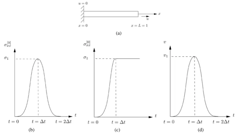
Figure 3(a)shows a schematic of the dimensionless rod of length one unit. The fixed end at x=0 is also the
[image:15.595.207.426.545.703.2](a)
[image:16.595.123.500.83.296.2](b) (c) (d)
Figure 3. Problem schematic, stress pulse, stress ramp, and velocity pulse loading. (a) Schematic; (b) Stress pulse loading: L1; (c) Stress ramp loading: L2; (d) Velocity pulse loading: L3.
origin of the x-frame. The dimensionless axial rod is of unit length. The right end of the rod (at x=1.0) is sub-jected to three different types of loading.
6.1. Loadings
We consider three different types of loads applied to the end of the rod at x=1.0.
Loading L1:
This loading consists of a stress pulse σxx[ ]0
( )
t of maximum amplitude ±σ1, positive for tensile loading andnegative for compressive loading applied over a time interval of 2∆t. In Figure 3(b), σ[ ]xx0
( )
t is continuouswith continuous first time derivative for 0≤ ≤ ∆t 2 t and is defined using the following.
[ ]
( )
[ ] [ ]( )
[ ] [ ]( )
[ ] [ ]( )
0 0 0 0 1 0 0 0at 0; 0, 0
at ; , 0
at 2 ; 0, 0
for 2 ; 0
xx xx xx xx xx xx xx t t t
t t t
t
t t t
t
t t t
σ σ σ σ σ σ σ σ ∂ = = = ∂ ∂ = ∆ = ± = ∂ ∂ = ∆ = = ∂ ≥ ∆ = (6.1)
The stress pulse σ[ ]xx0
( )
t described by (6.1) has support of 2∆t with maximum amplitude of ±σ1 att= ∆t such that for 0≤ ≤ ∆t 2 t σxx[ ]0
( )
t is a cubic function of time t and σ[ ]xx0( )
t =0 for t≥ ∆2 t.Loading L2:
This loading consists of stress σ[ ]xx0
( )
t defined as a ramp function over a time interval of ∆t with maximumvalue of [ ] ±σ1. Positive and negative signs correspond to tension and compression respectively. The ramp
( )
0
xx t
σ is continuous with continuous first derivative for 0≤ ≤ ∆t t and remains ±σ1 (constant magnitude)
for t≥ ∆t.
[ ]
( )
[ ] [ ]( )
[ ] [ ]( )
0 0 0 0 0 1 1at 0; 0, 0
at ; , 0 for ;
xx xx xx xx xx t t t
t t t t t t
t σ σ
σ
σ σ σ σ
The ramp σ[ ]xx0
( )
t described by (6.2) is a stress loading with maximum value of ±σ1 such that for0≤ ≤ ∆t t, σ[ ]xx0
( )
t is a cubic function of t with zero time derivatives at t=0 and at t= ∆t and a constantvalue of ±σ1 for t≥ ∆t. Figure 3(c)shows a schematic of this loading. Loading L3:
This loading (Figure 3(d)) consists of a velocity pulse, v t
( )
, of maximum amplitude ±v1, positive forten-sile loading and negative for compressive loading applied over a time interval of 2∆t. Similar to loading L1, we can define v t
( )
as follows.( )
( )
( )
( )
( )
( )
( )
1
at 0; 0, 0
at ; , 0
at 2 ; 0, 0
for 2 ; 0
v t
t v t
t v t
t t v t v
t v t
t t v t
t
t t v t
∂ = = = ∂ ∂ = ∆ = ± = ∂ ∂ = ∆ = = ∂ ≥ ∆ = (6.3)
The velocity v t
( )
described by (6.3) is a velocity pulse of support 2∆t with maximum amplitude of ±v1at t= ∆t. For 0≤ ≤ ∆t 2 t v t
( )
is a cubic function of t and v t( )
=0 for t≥ ∆2 t.6.2. Material Coefficients, Reference Quantities and Dimensionless Parameters
We define the material coefficients for thermoelastic sold continua and the thermoviscoelastic solid continua with and without memory, choice of reference quantities, and the resulting dimensionless material coefficients and the dimensionless variables and the parameters. The basic material is hard rubber or polymer which we would treat as thermoelastic, thermoviscoelastic without memory as well as with memory.
Thermoelastic Solid Continua (TE)
3 kg ˆ 1850 m ρ= 7 2 N
ˆ 1.49 10
m
E= ×
If we choose 0 1850 kg3 m
ρ = and 7
0 2
N 1.49 10
m
E = × as reference values, then the dimensionless density
0 0 ˆ 1 ρ ρ ρ = =
and the dimensionless modulus of elasticity 0
ˆ 1 E E E = = .
Thermoviscoelastic Solid without Memory (TVE)
3
kg J
ˆ 1850 ; ˆ 1650 kg K m cp
ρ = =
⋅
7 2
W N
ˆ 0.235 ; ˆ 1.49 10
m K m
k= E= ×
⋅
0 1 m; 0 300 K
L = θ =
reference speed of sound
0 0 0 0.0111 s L t v = = 2 2 0 ˆ ˆ ˆ ˆ ˆ E v E ρ ρ ρ = =
characteristic kinetic energy. If we choose
0 ˆ ,E0 Eˆ
ρ =ρ = , and cp0 =cˆp, then 0 0 ˆ 1 ρ ρ ρ = =
and 0
ˆ 1
E E
E
= = and 0 0 ˆ 1 p p p c c c = = .
Thermoviscoelastic Solid with Memory (TVEM)
The material coefficients, reference quantities, and dimensionless quantities and parameters for TVE hold here. Additionally for this solid continua we have Deborah number, De, defined by
0
De t λ
= . Numerical val-
ues of De used in the evolution computations are given with the details of studies. 6.3. Computations of Evolutions: Numerical Results
In the following sections we report numerical studies for loading L1 and L2 for TE, TVE, and TVEM solid con-tinua. Evolution in each case is computed using space-time strip with time marching until the desired value of time is reached. The choice of h, p, and k defining the scalar product space Hp k,
( )
Ωext containingspace-time local approximation function is important. Since all three mathematical models (dimensionless forms given by (4.1), (4.8), and (4.9)) are a system of first order partial differential equations in space coordinate x and time t, the choice of k=
(
k k1, 2) ( )
= 2, 2 in space and time ensures that the local approximations are of class C11 in space and time. Here the space-time integrals over n Txt
Ω , discretization of nth space-time strip n
xt
Ω are always Riemann. We consider a sixteen element uniform discretization of n xt
Ω giving rise to a spa-tial discretization length of 1/16. With E=1, ρ =0 1, the dimensionless wave speed is one, thus with ∆ =t 0.1,
the wave would be over a spatial domain of 0.1 which is spanned by approximately one and a half space-time element. Hence, at the onset, the sixteen element uniform spatial discretization
(
he =1 16)
appears to berea-sonable. With k=
(
k k1, 2) ( )
= 2, 2 and he=1 16, we need to conduct a p-convergence study to establish atwhat p-levels this choice of he is adequate to yield values of the residual functional for the space-time strip low
enough for the computed solution to be considered accurate or time accurate. For this purpose, we consider the first space-time strip with loading L2 and σ = ±1 0.01 and σ = ±1 0.1 at x=1.0 and ∆ =t 0.1. The p-levels
in space and time,
(
p p1, 2)
, are increased uniformly(
p= p1= p2)
from 3 to 11 in increments of 2. For eachp-level, a solution is computed using a tolerance ∆ =10−6 for gi ≤ ∆ =,i 1, 2, in Newton’s linear method
with line search. The behavior of the residual function I for 1 T
xt
Ω is examined as a function of the degrees of freedom for TE, TVE solids and for TVEM. Plots of residual function I versus degrees of freedom for TE, TVE, and TVEM for both linear and nonlinear cases corresponding to infintesimal (linear) and finite strain formulations (nonlinear) are given inFigure 4. In the mathematical models, f =0 is used for the linear case in which there is no non-linearity in any of the equations in the mathematical model. When f =1 (nonlinear case), the strain measure is Green’s strain and ρ
( )
x t, ≠ρ0( )
x , instead 0 1( )
,u
x t x
ρ =∂ + ρ
∂
holds due to the continuity equation. From the graphs in Figure 4, we note that: 1) in all three cases (TE, TVE, and TVEM) the residual I is of the order of O
(
10−12)
or lower for p= p1= p2 =9 or greater confirming that he =1 16,1 2 2
k =k = , and p1= p2 =9 are sufficient for accurate solution for the first space-time strip. For the second
[image:18.595.79.503.81.255.2]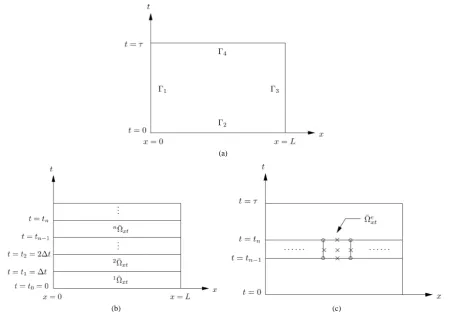


![Figure 5. Evolution of σ[ ]0xx along the length of the rod: TE, L1, Δt = 0.1, σ1 = −0.01](https://thumb-us.123doks.com/thumbv2/123dok_us/8071213.779646/20.595.74.543.79.692/figure-evolution-s-xx-length-rod-te-dt.webp)
![Figure 6. Evolution of σ[ ]0xx along the length of the rod: TE, L1, Δt = 0.1, σ1 = −0.01](https://thumb-us.123doks.com/thumbv2/123dok_us/8071213.779646/21.595.76.539.80.693/figure-evolution-s-xx-length-rod-te-dt.webp)
![Figure 7. Evolution of σ[ ]0xx along the length of the rod: TE, L1, Δt = 0.1, σ1 = −0.01](https://thumb-us.123doks.com/thumbv2/123dok_us/8071213.779646/23.595.77.540.77.689/figure-evolution-s-xx-length-rod-te-dt.webp)
![Figure 8. Evolution of σ[ ]0xx along the length of the rod: TE, L2, Δt = 0.1, σ1 = −0.01](https://thumb-us.123doks.com/thumbv2/123dok_us/8071213.779646/24.595.80.540.78.687/figure-evolution-s-xx-length-rod-te-dt.webp)
![Figure 9. Evolution of σ[ ]0xx along the length of the rod: TE, L2, Δt = 0.1, σ1 = −0.01](https://thumb-us.123doks.com/thumbv2/123dok_us/8071213.779646/25.595.76.540.78.694/figure-evolution-s-xx-length-rod-te-dt.webp)
