PLACEMENT AND SIZING OF DISTRIBUTED GENERATORS IN DISTRIBUTED NETWORK BASED ON LRIC AND LOAD GROWTH CONTROL

ARCHITECTURE OPTIMIZATION MODEL FOR THE

MULTILAYER PERCEPTRON AND CLUSTERING

1_{Mohamed ETTAOUIL,} 2_{Mohamed LAZAAR and} 3_{Youssef GHANOU}

1,2 _{Modeling and Scientific Computing Laboratory, Faculty of Science and Technology, University Sidi}

Mohammed Ben Abdellah, Fez, Morocco

3_{High School of Technology, University Moulay Ismail Meknes, Morocco}

E-mail: 1mohamedettaouil@yahoo.fr

,

ABSTRACT

This paper presents an approach called Architecture Optimization Model for the multilayer Perceptron. This approach permits to optimize the architectures for the multilayer Perceptron. The results obtained by the neural networks are dependent on their parameters. The architecture has a great impact on the convergence of the neural networks. More precisely, the choice of neurons in each hidden layer, the number of hidden layers and the initial weights has a great impact on the convergence of learning methods. In this respect, we model this choice problem of neural architecture in terms of a mixed-integer problem with linear constraints. We propose the genetic algorithm to solve the obtained model. The experimental work for classification problems illustrates the advantages of our approach.

Keywords: Multilayer Perceptron, Non-linear optimization, Genetic algorithms, Supervised Training,

Clustering.

1. INTRODUCTION

The Artificial Neural Networks (ANN) are a very powerful tool to deal with many applications, and they have proved their effectiveness in several research areas such as analysis and image compression, recognition of writing, speech recognition [2], signal analysis, process control, robotics, and research on the Web [14] [12].

An artificial neural network is an information-processing system that has certain performance characteristics in common with biological neural networks. Artificial neural networks have been developed as generalizations of mathematical models of neural biology [14], based on the assumptions that:

- Information processing occurs at many simple elements called neurons.

- Signals are passed between neurons over connection links.

- Each connection link has an associated weight, which, in a typical neural network, multiplies the signal transmitted.

- Each neuron applies an activation function to its network input to determine its output signal.

Optimizing the number of hidden layer neurons for establishing a multilayer Perceptron to solve the problem remains one of the unsolved tasks in this research area Multilayer Perceptron consists of input layer, output layer and hidden layers between these two layers. The number of these layers is dependent on the problem [16] [3]. In this work, we optimize the number of hidden layers and the number of neurons in each hidden layer to increase the speed and efficiency of the neural network [6]. To optimize these hidden layers and neurons of the multilayer Perceptron, we model this problem of neural architecture in terms of a mixed-integer non linear problem with linear constraints.

In this paper, we model this problem as mixed-integer non lineaire programming. We apply genetic algorithms to find the optimal number of hidden layers, the activation function and the initial matrix of weights. We formulate this problem as a non linear programming with constraints. Genetic algorithm is proposed to solve it. Consequently we determine the optimal architecture and the initial matrix of weights.

2. MULTILAYER PERCEPTRONS

theoretical and experimental artificial neural net models which he proposed in the period 1957-1962. Rosenblatt's work created much excitement, controversy, and interest in neural net models for pattern classification in that period and led to important models abstracted from his work in later years. Currently the names (single-layer) Perceptron and Multilayer Perceptron are used to refer to specific artificial neural network structures based on Rosenblatt's perceptrons [20].

In artificial neural network consists of a series of nodes (neurons) which have multiple connections with other nodes. Each connection has a weight associated with it which can be varied in strength, in analogy with neurobiology synapses. A typical ANN architecture known as a multilayer perceptron(MLP). The principal with which a neural network operates is relatively simple. Each neuron in the input layer holds a value, so that the input layer holds the input vector. Each of these neurons connects to every neuron in the next layer of neurons.

The architecture of an Artificial Neural Network is a layout of neurons grouped in layers. The main parameters of ANN: number of layers, number of neurons per layer, connectivity level and type of neurons interconnectors [17][21].

A multilayer Perceptron (MLP) is a variant of the original Perceptron model proposed by Rosenblatt in the 1950 [19]. It has one or more hidden layers between its input and output layers, the neurons are organized in layers, the connections are always directed from lower layers to upper layers, the neurons in the same layer are not interconnected.

The first layer of the neural network is the input layer, we assume it contains n neurons, the last layer of the network is the output layer, we assume it contains m neurons.

In the Perceptron model, a single neuron with a linear weighted net function and a threshold activation function is employed. The input to this neuron is a feature vector in an n-dimensional feature space. The net function is the weighted sum of the inputs:

Input Layer: A vector of predictor variable

values is presented to the input layer. The input layer distributes the values to each of the neurons in the first hidden layer.

Hidden Layer: A group of neurons between an

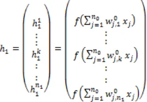
input layer and output layer. The outputs from the hidden layer are distributed to the output layer. The neurons of first hidden layer are directly connected to the input layer (data layer) of the neural network; Figure 1 shows the connections between the first hidden layer and the inputs of the network.

Figure 1. Outputs For The First Hidden Layer

To calculate the outputs for the first hidden layer, we use the following:

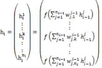
Figure 2 Shows The Connections Between The I-1 Hidden Layer And The I Hidden Layer Of The Neural

Network.

x

x

x

x

Figure 2. Outputs For The Hodden Layer I=2,…,N

The outputs of the hidden layer i for i=2,…,N can calculate by the role:

: The weight between the neuron j for the layer i-1 and the neuron k for the layer i.

: Activation function.

Output Layer: Arriving at a neuron in the output layer. The connections between the last hidden layer and Output layer of the neural network are show in Figure 3.

The outputs Y of the network are calculated by this following:

Figure 3. Outputs For The Neural Network

The network can have any number of hidden layers. The values on the output layer of neurons are the outputs from the network.

A. Learning Techniques

Learning is a process by which the free parameters of a neural network are adapted through a continuing process of stimulation by the environment in which the network is embedded. The type of learning is determined by the manner in which the parameter changes take place. The multilayer perceptron is a supervised learning.

Supervised training takes place as follows. The weights are initially set random values over a small range. When a vector is fed into the network, the output vector will also be random. By comparing this output with what it should be, we can perturb the weights to give an output which is closer to the target value. This is repeated for each vector in the training data set. The network is trained iteratively by successive passes of the training data though the network.

There are various schemes for training the network in this fashion, but one of the mots common and successful is the back-propagation [17].

B. Backpropagation

Backpropagation neural network [23] architecture is the most popular supervised learning networks. Their topology allows the data to flow in the same direction along the network using a technique called error Backpropagation. It makes possible to readjust the connection weights.

Forward Phase: During this phase the free parameters of the network are fixed, and the input hidden layer i-1 Hidden layer i

signal is propagated through the network layer by layer. The forward phase finishes with the computation of an error signal:

where di is the desired response and yi is the

actual output produced by the network in response to the input xi.

Backward Phase: During this second phase, the error signal ei is propagated through the network in

the backward direction, hence the name of the algorithm. It is during this phase that adjustments are applied to the free parameters of the network so as to minimize the error ei in a statistical sense.

This sort of network has to be made of one Input Layer and one Output Layer, between these both layers, least one hidden layer. Hidden layers propagate the information along the networks.

3. OPTIMIZATION OF ARTIFICIAL

NEURAL ARCHITECTURE

The problem of neural architectures optimization is to find the optimal number of hidden layers in the ANN, the number of neurons within each layer, and the good activation function, in order to maximize the performance of artificial neural networks [5][6][8]. In this work, we assign to each neuron a binary variable which takes the value 1 if the neuron is active and 0 is otherwise.

Notation:

: Number of hidden layers.

: Number of neurons in input layer.

: Number of neurons in hidden layer i.

: Optimal number of neurons in hidden layer i.

: Number of neurons in output layer.

: Input data of neural network.

: Calculated output of neural network.

: Output of neuron j in hidden layer i.

: Activation function.

: Desired output.

: Binary variable for and .

where

We computed the output of neural network by the following formulation:

- Output of first hidden layer

The neurons of first hidden layer are directly connected to the input layer (data layer) of the neural network; Figure 1 shows the connections between the first hidden layer and the inputs of the network.

The output for each neuron in the first hidden layer is calculated by:

- Output for the hidden layer i = 2,…,N

The number of hidden layer and number of neurons in each layer has a great impact on the convergence of the learning for the multilayer neural network.

- Output for the neural network

The output of the neural network is defined by the following expression:

Objective function

The objective function of the proposed model is the error between the calculated output and desired output:

Constraints

The last constraints guarantee the existence of the hidden layers.

Optimization Model

The neural architecture optimization problem can be formulated as the following model:

Let presents the solution of the optimization problem (P).

Many exact methods for solving mixed-integer non-linear programming (MINLPs) include innovative approaches and related techniques taken and extended from Mixed-integer programming (MIP). Outer Approximation (OA) methods [6] [10], Branch-and-Bound (B&B) [12] [18], Extended Cutting Plane methods [22], and Generalized Bender’s Decomposition (GBD) [10] for solving MINLPs have been discussed in the literature since the early 1980’s. These approaches generally rely on the successive solutions of closely related NLP problems. For example, B&B starts out forming a pure continuous NLP problem by dropping the integrality requirements of the discrete variables (often called the relaxed MINLP or RMINLP). Moreover, each node of the emerging B&B tree represents a solution of the RMINLP with adjusted bounds on the discrete variables [1].

The disadvantage of the exact solution methods mentioned above is that they become computationally intensive as the number of variables is increased throughout the procedure. Therefore, efficient heuristic methods are required to solve large-size instances accurately.

The heuristics methods for solving combinatorial optimization have now a long history, and there are virtually no well-known, hard optimization problems for which a meta-heuristic has not been applied. Often, meta-heuristics obtain the best known solutions for hard, large-size real problems, for which exact methods are too time consuming to be applied in practice.

4. SOLVING THE OBTAINED

OPTIMIZATION MODEL USING GENETIC ALGORITHM

In this section, we use the genetic algorithm to solve the architecture optimization problems. To this end, we have coded individual by tree chromosomes; moreover, the fitness of each individual depends on the value of the objective function.

optimization problems in several domains, telecommunication, routing, scheduling, and it proves it's efficiently to obtain a good solution [3]. We have formulated the problem as a non linear program with mixed variables [13].

Genetic algorithm

1. Choose the initial population of individuals; 2. Evaluate the fitness of each individual in that

population;

3. Repeat on this generation:

a. Select the best-fit individuals for reproduction;

b. Crossover and Mutation operations; c. Evaluate the individual fitness of new

individuals;

d. Replace least-fit population with new individuals;

Until termination (time limit, fitness achieved).

A. Initial population

The first step in the functioning of a GA is the generation of an initial population. Each member of this population presents a feasible solution of the problem.

The individual of the initial population are randomly generated, and take the value 0 or 1, and the weights matrix takes random values in

space where and

where

. Because all the observations are in the set .

B. Evaluating individuals

After creating the initial population, each individual is evaluated and assigned a fitness value according to the fitness function.

In this step, each individual is assigned a numerical value called fitness which corresponds to its performance; it depends essentially on the value of objective function in this individual. An individual who has a great fitness is the one who is the most adapted to the problem.

The fitness suggested in our work is the following function:

Minimize the value of the objective function is equivalent to maximize the value of the fitness function.

C. Selection

The application of the fitness criterion to choose which individuals from a population will go on to reproduce.

Where

D. Crossover

The crossover is very important phase in the genetic algorithm, in this step, new individuals called children are created by individuals selected from the population called parents. Children are constructed as follows:

We fix a point of crossover, the parent are cut switch this point, the first part of parent 1 and the second of parent 2 go to child 1 and the rest go to child 2.

In the crossover that we adopted, we choose 2 different crossover points, the first for the matrix of weights and the second is for vector U.

E. Mutation

The rule of mutation is to keep the diversity of solutions in order to avoid local optimums. It corresponds on changing the values of one (or several) value (s) of the individuals who are (or were) (s) chosen randomly.

5. EXPERIMENT RESULTS

Classification algorithms attempt to organize unlabeled feature vectors into clusters such that points within a cluster are more similar to each other than to vectors belonging to different clusters.

Table I :Experiments Results

Pm Pc {n1,n2} {n1,op ,n2,op}

0.2 0.8 {8,8} {3,4}

0.3 0.8 {7,7} {4,4}

0.3 0.7 {10,10} {3,3}

0.3 0.7 {9,9} {4,4}

Where:

- Pm: Probability of mutation - Pc: Probability of crosser

- ni: number of neurons in hidden layer i. - ni,op : optimal number of neurons

determined using the proposed method in hidden layer i.

After determining the optimal number of neurons in each hidden layer and the hidden layers, we can initialize the neural networks by an adequate number of neurons. Our algorithm tested on instances for Iris data. We use an architecture contains two hidden layers, in each layer four neurons.

Table II :Classification For Training Data

Nr. T.

D. C.C MC

Accuracy (%)

Setosa 25 25 0 100

Virginica 25 25 1 96

Versicolor 25 23 2 92

Overall 75 73 3 97.3

Where Nr. T. D. is the Number of Training Data and C. C. is the data Correctly Classified.

The TABLE II presents the obtained clustering results of training data. We remark that the proposed method permits to classify all the training data only three data; one from Virginica and two from Versicolor.

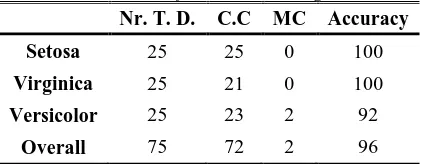
Table IIII: Classification For Testing Data

Nr. T. D. C.C MC Accuracy

Setosa 25 25 0 100

Virginica 25 21 0 100

Versicolor 25 23 2 92

Overall 75 72 2 96

The TABLE III presents the obtained clustering results of testing data. This table shows that our

method gives the good results, because all the testing data were correctly classified except two. In fact; these elements (misclassified) are from the Versicolor class.

A comparison of the average classification accuracy rate of the proposed method with other existing neural networks training algorithms: Error Back-Propagation (EBP), Radial Basis Function (RBF) neural networks and Support Vector Machine (SVM). We use half of the data examples (75 items) for training and the remaining (75 items) for testing as well.

Table III: Comparison For Iris Data Classification

Method CPU It. M.T. M.TS A.T

(%)

A.TS (%) EBP 39.98 500 3 2 96 97.3

EBP 68.63 800 2 1 97.3 98.6

RBF 16.84 85 4 4 94.6 94.6

RBF 19.81 111 4 2 96 97.3

SVM 8.743 5000 3 5 94.6 93.3

Proposed

Method 11.35 100 3 2 96 97.3

- It: Number of iterations;

- M.T.: Misclassified for training set; - M.TS.: Misclassified for testing set; - A.T.: Accuracy for training set; - A.TS.: Accuracy for testing set.

The results are shown in the TABLE IV, we can see that the proposed method gets a higher average classification accuracy rate than the existing methods.

In addition, the number of hidden neurons must be decided before training in both EBP and RBF neural networks. Different number of hidden neurons results in different training time and training accuracy. It is still a difficult task to determine the number of hidden neurons in advance.

6. CONCLUSION

A Model is developed to optimize the architecture of Artificial Neural Networks. The Genetic Algorithm (GA) is especially appropriate to obtain the optimal solution of the nonlinear problem. This method is tested to determine the optimal number of artificial neurons in the Multilayer Perceptron and the most favorable weights matrix. We have proposed a new modeling for the multilayer Perceptron architecture optimization problem as a mixed-integer problem with constraints. The aim is to obtain optimal number of hidden layers and the optimal number of neurons in each hidden layer depending on the Iris data, the results obtained demonstrates the good generalization of neural networks architectures. In conclusion, the optimal architecture of artificial neural network can play an important role in the classification problem. We can call the proposed approach to solve many other problems; speech, image, robotics,

REFERENCES

[1] J. F. Benders, “Partitioning procedures for solving mixed-variables programming problems”. Numer. Math., 4:238, 1962.

[2] M. K. Apalak, M. Yildirim, R Ekici, “Layer optimization for maximum fundamental frequency of laminated composite plates for different edge conditions”, composites science and technology (68), 2008, pp. 537-550. [3] K. Deep, K. Pratap Singh, M.L. Kansal, C.

Mohan, “A real coded genetic algorithm for solving integer and mixed integer optimization problems”, Applied Mathematics and Computation, 2009, pp. 505–518.

[4] L. Derong, C. Tsu-Shuan, Z. Yi, “A Constructive Algorithm For Feedforward Neural Networks With Incremental Training”, IEEE Transactions on circuits and systems-I: fundamental theory and applications, Vol. 49, No. 12, 2002.

[5] M. Duran, I. E. Grossmann. “An outer-approximation algorithm for a class of mixed-integer non linear programs”. Mathematical Programming, 1986, pp. 307-339.

[6] E. Egriogglu, C, Hakam Aladag, S. Gunay, “A new model selection straegy in artificiel neural networks”, Applied Mathematics and Computation (195), 2008, pp. 591-597.

[7] M. Ettaouil and Y. Ghanou, “Neural architectures optimization and Genetic

algorithms”, Wseas Transactions On Computer, Issue 3, Volume 8, 2009, pp. 526-537.

[8] M. Ettaouil, Y.Ghanou, K. Elmoutaouakil, M. Lazaar, “A New Architecture Optimization Model for the Kohonen Networks and Clustering”, Journal of Advanced Research in Computer Science (JARCS), Volume 3, Issue 1, 2011, pp. 14 - 32.

[9] M. Ettaouil, C. Loqman. “A New Optimization Model for Solving the Constraint Satisfaction Problem”. Journal of Advanced Research in Computer Science (JARCS). Volume 1, Issue 1, 2009, pp. 13 - 31.

[10]R. Fletcher and S. Leyffer, “Solving Mixed Integer Programs by Outer Approximation”, Math. Program. 66, 1994, pp. 327–349.

[11]J. A. Freeman, D. M. Skapura, “Neural Networks Algorithms, Applications and Programming Techniques”, Pearson Education, 2004, pp. 213 – 262.

[12]O.K. Gupta and A. Ravindran, “Branch and Bound Experiments in Convex Nonlinear Integer Programming”, Manage Sci., 31 (12), 1985, pp. 1533–1546.

[13]Hasham Shiraz Ali, Umar Nauman, Faraz Ahsan, Sajjad Mohsin, “Genetic Algorithm Based Bowling Coach For Cricket”, Journal of Theoretical and Applied Information Technology, Vol 37. No. 2, 2012, pp 171-176. [14]J.Hertz, A. Krogh, and R.G. Palmer,

“Introduction to Theory of Neural Computation”. Santa Fe Institute Studies in the Sciences of Complexity. Addison Wesley, Wokingham, England, 1991.

[15]J. Holland, “Genetic Algorithms”, pour la science, n°179, Edition of Scientific American, 1992, pp. 44-50.

[16]T.Y. Kwok, D.K. Yeung, “Constructive algorithms for structure learning in feed forward neural networks for regression problems”, IEEE Trans. Neural Networks 8, 1997, pp. 630-645.

[17]X. Liang, “Removal of hidden neurons in multilayer perceptrons by orthogonal projection and weight crosswise propagation”, Neural Comput. & Applic., 16, 2007, pp. 57-68.

[19]Rosenblatt, “The Perceptron: A Theory of Statistical Separability in Cognitive Systems”, Cornell Aeronautical Laboratory, Report No. VG-1196-G-1, January, 1958.

[20]F. Rosenblatt, “Perceptrons and the Theory of Brain Mechanisms”, Cornell Aeronautical Laboratory, Report No. VG-1196-G-8. September, 1960.

[21]A. C. Subhajini, T. Santhanam, “Fuzzy Artmapneural Network Achitecture For Weather Forecasting”, Journal of Theoretical and Applied Information Technology, Vol 34. No. 1, 2011, pp 022-028.

[22]T.Westerlund and F. Petersson, “A Cutting Plane Method for Solving Convex MINLP Problems”, Computers Chem. Eng., 19, 1995, pp. 131–136.