PARIS RESEARCH LABORATORY
d i g i t a l
March 1993 J ´er ˆome Barraquand
Numerical Valuation
of High Dimensional Multivariate
European Securities
J ´er ˆome Barraquand
The author can be contacted at the following address:
J´erˆome Barraquand
Digital Equipment Corporation Paris Research Laboratory 85, avenue Victor Hugo 92563 Rueil-Malmaison Cedex France
c
Digital Equipment Corporation 1993
We consider the problem of pricing a contingent claim whose payoff depends on several sources of uncertainty. Using classical assumptions from the Arbitrage Pricing Theory, the theoretical price can be computed as the discounted expected value of future cash flows under the modified risk-neutral information process. Although analytical solutions have been developed in the literature for a few particular option pricing problems, computing the arbitrage prices of securities under several sources of uncertainty is still an open problem in many instances. In this paper, we present efficient numerical techniques based upon Monte Carlo simulation for pricing European contingent claims depending on an arbitrary number of risk sources. We introduce in particular the method of quadratic resampling (QR), a new powerful error reduction technique for Monte Carlo simulation. Quadratic resampling can be efficiently combined with classical variance reduction methods such as importance sampling to further improve the accuracy of the estimate. Our numerical experiments show that the method is practical for pricing claims depending on up to one hundred underlying assets. We also describe an implementation of the method on a massively parallel supercomputer, yielding two orders of magnitude of performance improvement over the same implementation on a desktop workstation.
R ´esum ´e
Finance, arbitrage, pricing, options, multidimensional contingent claim, Monte Carlo method, importance sampling, quadratic resampling, massively parallel computing
Acknowledgements
1.1 Background : : : : : : : : : : : : : : : : : : : : : : : : : : : : : : : : 1 1.2 Multidimensional pricing models : : : : : : : : : : : : : : : : : : : : : 1 1.3 European versus American instruments : : : : : : : : : : : : : : : : : 3
2 Relation to other work 5
3 Arbitrage pricing of European securities 7
3.1 Diffusion model of information process : : : : : : : : : : : : : : : : : 7 3.2 European securities : : : : : : : : : : : : : : : : : : : : : : : : : : : : 8 3.3 Arbitrage Pricing : : : : : : : : : : : : : : : : : : : : : : : : : : : : : : 9
4 Monte Carlo valuation 10
4.1 Numerical integration on the real line : : : : : : : : : : : : : : : : : : 10 4.2 Multidimensional integration : : : : : : : : : : : : : : : : : : : : : : : 11 4.3 Monte Carlo method and importance sampling : : : : : : : : : : : : : 13 4.4 Quasi-random sampling : : : : : : : : : : : : : : : : : : : : : : : : : : 15
5 Quadratic resampling 17
6 Experimental results 20
6.1 A test case : : : : : : : : : : : : : : : : : : : : : : : : : : : : : : : : : 20 6.2 Comparison with classical Gaussian rules : : : : : : : : : : : : : : : 26 6.3 Massively parallel implementation : : : : : : : : : : : : : : : : : : : : 28
7 Conclusion 30
1 Introduction
1.1 Background
Since the seminal work of Black and Scholes [Black and Scholes, 73] and Merton [Merton, 73] in the early 1970s, the arbitrage principle underlying option valuation theory has been extended to a broad range of other financial instruments (see e.g. [Ross, 76], [Cox and Rubinstein, 85]). Indeed, any security whose returns are contractually related to the returns on some other security or group of securities can theoretically be valuated using the same arbitrage principle. This is the case in particular of warrants, convertible bonds, but also common stocks, ordinary bonds, and most other types of contractual instruments. In some cases, explicit closed form analytical formulas for the computation of the arbitrage price can be derived from this theory. In particular, the original paper of Black and Scholes provides a closed form solution for a European option on a single common stock. Unfortunately, few other cases can be solved analytically, and computing the arbitrage price often requires numerical simulations. Following an idea initially presented in an early edition of [Sharpe, 85], Cox, Ross, and Rubinstein [Cox, Ross, and Rubinstein, 79] [Cox and Rubinstein, 85] developed a discrete model for the valuation of an American option on a single stock that can be easily computed numerically. However, the effective implementation of the arbitrage principle is not always such an easy task, and may sometimes become intractable. For example, when a contingent claim depends on many sources of uncertainty, there is no known general tractable algorithm for computing accurately the arbitrage price.
1.2 Multidimensional pricing models
There are several reasons motivating the development of efficient methods for multidimensional contingent claim pricing. We briefly review some of them below, but the list is certainly not exhaustive. The tremendous development of financial engineering during the past decade can be expected to continue, and new types of securities requiring multidimensional modeling are likely to appear at a sustained pace in the future.
Complex Over The Counter warrants
Many instruments depending on several underlying securities are being proposed on Over The Counter markets. One can buy options on the best performance of several securities, or on the spread between different market indexes. In foreign exchange markets, complex instruments are being proposed that enable investors to diversify their portfolios internationally while protecting them from the relative variations of several different currencies. In commodity markets, long-dated options on portfolios of futures contracts with various maturities are being proposed to protect investors from long term evolutions of the underlying commodity and of its convenience yield.
Specialized institutions are now proposing options that depend not only on the current value of the underlying asset, but on the whole history of underlying asset prices until expiration date. Well known examples are lookback options (e.g. options on the minimum value of the underlying for a given period of time), and Asian options (e.g. options on the average value of the underlying for a given period of time). These path-dependent instruments can be viewed as multidimensional contingent claims on the sequence of underlying asset prices until the expiration date. Other examples of path-dependent instruments are Mortgage-Backed Securities (MBS), which depend on the past history of interest rates, and certain life insurance contracts, such as Single Premium Deferred Annuities (SPDA) and Guaranteed Interest Contracts (GIC).
Interest rate related instruments
A new generation of term structure models [Heath, Jarrow, and Morton, 92] has recently been developed. These models can account for non-parallel evolutions of the term structure, i.e. discrepancies in the evolutions of short and long-term rates. According to these models, the whole term structure of interest rate is a multidimensional underlying asset for interest rate contingent claims. Examples of interest rate contingent claims include all kinds of fixed-income securities such as bonds and convertible bonds, bond options, swaps, caps, floors, collars, swaptions, but also mortgage-backed securities and SPDAs [Fabozzi, 87].
Models with stochastic parameters
Is is well known that the volatility of the underlying asset cannot be assumed constant for long-term options. Recently, new option pricing models have been developed that attempt to take into account the stochastic nature of volatility (see e.g. [Wiggins, 87], [Dothan, 87], [Hull and White, 88]). In these models, the option price depends on two sources of uncertainty: the underlying asset itself, and its volatility. Similarly, the interest rates cannot be assumed constant for a long period of time. Therefore, pricing long-dated options requires modeling the uncertainty arising for interest rate variations. Examples of commodity or stock option pricing models accounting for uncertainties in stochastic interest rates can be found in [Merton, 73], [Jarrow, 87]. Of course, as described above, fixed income securities and related derivative instruments also require modeling of the stochastic nature of interest rates. More generally, any parameter in the stochastic model of the underlying asset that cannot be assumed predictable constitutes a new source of uncertainty that cannot be neglected for long-dated instruments.
Quality delivery options in futures contracts
Pricing of insurance contracts
The Arbitrage Pricing Theory can be applied to the pricing of insurance policies. In particular, as described above, some life insurance policies can be viewed as pure interest rate contingent claims (see e.g. [Stanton, 89]). More generally, option pricing theory can be applied to the valuation of property/liability insurance contracts, where the strike price of the option corresponds to the deductible of the insurance policy. There is a growing academic literature on these subjects, that can be traced back to the work of [Merton, 77] and [Smith, 79]. Other applications are presented in [Kraus and Ross, 82], [Doherty and Garven, 86], [Cummins, 88] [Shimko, 92].
Assets and Liabilities Management
Large corporations bear many different kinds of risks in the course of their activities. Some of these risks can be hedged on financial markets. In particular, the currency exchange risks and the interest rate risks can be hedged in many cases. For financial institutions such as major banks and life insurance companies, this financial risk is the only major source of uncertainty of the business. In order to minimize this risk, the corporation must immunize itself as much as possible against variations of the economic value of the firm as a function of the sources of uncertainty. This economic value is simply the difference between the present value of assets and the present value of liabilities. Given a model of the commercial and financial policy of the firm, these present values can be computed as contingent claims on the economic variables representing the risk (e.g. interest rates and currency exchange rates).
Capital budgeting models in corporate investment decision making
When assessing the opportunity to invest in a new project, a financial manager must determine the Net Present Value (NPV) of the project, i.e. the economic value of all the possible future cash flows generated by the project. Several economic and commercial variables are generally relevant for building a model of the probability distribution of the future cash flows. In particular, when building the business plan for introducing a new product to the market, one must estimate the possible evolutions of the parameters associated with the product, as functions of the predefined marketing policy. These parameters can be the market size, the market share of the company, the fixed and variable costs, the expected price. Also, global economic variables such as gross national product, rate of inflation, or interest rates may be relevant. According to [Brealey and Myers, 91], the net present value can be computed as the expected value of all future cash flows, discounted at the opportunity cost of capital. Computing the NPV can be viewed as pricing a multidimensional contingent claim on the relevant economic and commercial parameters. See [Mason and Merton, 85] for a review of applications of option pricing theory to corporate finance.
1.3 European versus American instruments
after the purchase date. Most assets traded on financial markets belong to this class. We will call European instruments all financial assets belonging to this first class. In particular, stocks, bonds, futures contracts, European options, swaps, caps, floors, mortgage-backed securities are European instruments. The second class is that of assets whose cash flows can be influenced a posteriori by the holder. American options belong to this class. As another example, the crediting policy of a Life Insurance company selling SPDAs greatly influences the present value of the liabilities of the company. This crediting policy can be adjusted by the company after signature of the contracts with the policyholders. Therefore, the liability associated with the sale of SPDA can be viewed as an American security. We will call American instruments all financial assets belonging to this second class.
Following the general theory of arbitrage pricing, the theoretical price of a European contingent claim is the discounted expected value of its future cash flows under the so-called “risk-neutral” probability distribution of the underlying economic factors [Harrison and Kreps, 79] [Harrison and Pliska, 81], [Duffie, 88], [Karatzas and Shreve, 88]. Mathematically, computing the arbitrage price reduces to computing an integral (sum) over the space of the underlying economic factors. When the dimension of the space of the underlying economic factors is small, standard techniques for numerical integration can be used. In some cases, the integral can even be computed analytically (e.g. Black-Scholes formula). However, the computational complexity of evaluating the integral is clearly exponential in the dimension of the space.
In this paper, we present efficient numerical techniques based upon Monte Carlo simulation that enable us to compute accurate approximations of realistic European pricing problems in a time quadratic in the number of underlying economic factors. Combining classical techniques of importance sampling with a new approximation method called quadratic resampling, we can compute the theoretical prices of the most complex instruments within tens of seconds on a PC or a workstation, and within a fraction of a second on currently available massively parallel supercomputers. The method has been tested for pricing problems with up to 100 underlying factors.
This paper is organized as follows. In Section 2, we relate our contribution to previous work in Monte Carlo integration and asset pricing. In Section 3, we recall the usual assumptions on the stochastic processes governing the evolution of securities prices, and the main result of the Arbitrage Pricing Theory. In Section 4, we briefly review Monte Carlo techniques for the numerical valuation of multidimensional integrals, and describe in particular modern importance sampling methods. In Section 5, we present the method of quadratic resampling. In Section 6, we present numerical results demonstrating the efficiency of the quadratic resampling method when combined with appropriate importance sampling schemes. We also describe a massively parallel implementation of our Monte Carlo procedure. Finally, in Section 7, we discuss the capabilities and limitations of the approach.
2 Relation to other work
Good reviews of the Monte Carlo method and different variance reduction techniques such as antithetic variables, covariates, stratified sampling, importance sampling can be found in many sources such as [Hammersley and Handscomb, 64], [Zaremba, 68], [Haber, 70], [Kalos and Whitlock, 86], [Decker, 91] and references thereof. [Stroud, 71] is a comprehensive source of results regarding multidimensional Gaussian quadrature rules. All our experiments on Gaussian rules are based on methods proposed in [Stroud, 71]. The additive importance sampler presented in this paper is described in [Dantzig and Glynn, 89] and [Dantzig and Infanger, 91] in the context of portfolio optimization and other operations research applications.
The application of the Monte Carlo method to option pricing was first presented in [Boyle, 77], in the context of claims contingent to a single underlying asset. It has then been used by several authors for the valuation of path dependent contingent claims. In particular, the method has been used for pricing mortgage-backed securities (see [Schwartz and Torous, 89], [Hutchinson and Zenios, 91]). Interestingly, the model described in [Schwartz and Torous, 89] could be solved faster by direct finite-difference approximation of the arbitrage partial differential equation. Indeed, although the problem is initially path-dependent as a function of interest rates, it can be made path-independent by including two additional state variables in the model. These new variables aggregate all the necessary information on past values of interest rates. The final model is four-dimensional, which is still tractable for direct numerical integration. This technique of including new state variables to remove path dependence is described in much detail in [Stanton, 89]. Many problems of path-dependence can be solved that way. The Monte Carlo method, although much slower than direct numerical integration for problems with few dimensions, is very flexible and simple to implement. This is why it has been used in many problems of path-dependence that could be solved faster by direct numerical integration. Another application of the Monte Carlo method to the valuation of Single Premium Deferred Annuities contracts is described in [Stanton, 89].
interest rates. The approach is clearly limited to a few assets, since the memory space requirements and the computation time are both exponential in the number of underlying assets. [Boyle, Evnine, and Gibbs 89] developed a multinomial lattice method for pricing multidimensional options, in the spirit of the approach outlined in [Cox and Rubinstein, 85]. According to the authors, the computation becomes very burdensome for more than two assets. In fact, the multinomial lattice approach can be viewed as a finite-difference approximation of the generalized Black-Scholes equation using an explicit Euler scheme and an appropriate change of variables [Brennan and Schwartz, 78].
[Stulz, 82] presents an analytical solution to the problem of pricing a European option on the maximum or minimum of two underlying assets. The analytical solution is generalized in [Johnson, 87] to the case of an arbitrary number of assets, taking as given the cumulative multivariate normal distribution function. [Boyle, 89] and [Boyle and Tse, 90] developed an approximate method for the same problem. Although the problem is solved analytically in [Johnson, 87], the approximate method does not require preliminary computation of the cumulative multivariate normal distribution function. To the best of our knowledge, the above problem of option pricing on the maximum or minimum of several assets is the only case reported in the literature where solutions to high-dimensional (say, more than 5) problems have been developed.
Our contribution to the problem of multidimensional contingent claim pricing reported in this paper is twofold:
–First, we show that a proper implementation of the Monte Carlo method makes the problem of European contingent claims pricing tractable, even when the number of underlying assets is very large (up to 100 in our experiments).
–Second, we present a set of three techniques for improving the accuracy of the Monte Carlo estimation.
We introduce an original error reduction technique, quadratic resampling, that consider-ably improves the accuracy of Monte Carlo integration. Quadratic resampling can be used for any multidimensional integration problem, and is computationally practical for integrals with up to a few hundred dimensions. It can be combined with classical vari-ance reduction techniques such as importvari-ance sampling to further improve the accuracy of the computation. It is shown that, given a random vector having arbitrarily many coordinates and an arbitrary joint distribution, the expected value of any polynomial of degree two or less in the vector coordinates is computed exactly when using quadratic resampling.
We show that with currently available massively parallel technology, multidimensional contingent claim prices can be computed two orders of magnitude faster than on a desktop workstation. Therefore, since the accuracy of the Monte Carlo estimate is proportional to the square root of the number of samples, the massively parallel implementation is one order of magnitude more accurate than the workstation implementation for a given computing time.
3 Arbitrage pricing of European securities
The arbitrage pricing theory is described in many textbooks. We refer the reader to [Duffie, 92] for a comprehensive presentation.
3.1 Diffusion model of information process
We model the economy as a finite-dimensional vector of real-valued state variables X(t)= (x1(t);. . .;xn(t)), called factors, representing all the information available to investors at time t. By definition, X(t)is known at time t. However, X(t)does not usually give enough information to investors to allow perfect forecasting of the future evolutions of security markets. Therefore, X(); >t is a stochastic process.
By construction, X(t)is a Markov process, i.e. future values of vector X are independent of past values of vector X, conditionally to the knowledge of X today. Indeed, if future values of
X were to depend not only on X(t)but also on past values, this would mean that X(t)does not represent all relevant information at time t, contradicting its definition.
Since X(t)represents all information available to agents at time t, in a frictionless market, prices of securities must be deterministic functions of time and X(t). It is said that securities are contingent claims on the state variable X(t).
For the sake of simplicity, we will assume that the information process X(t)is a diffusion
process. However, our results on Monte Carlo valuation described in the next sections apply
to more general types of stochastic processes. If X(t)is a diffusion process, it is a solution of a stochastic differential equation of the type:
dX=A(X(t);t)dt + B(X(t);t)dW (1)
or equivalently:
8i2[1;n]; dxi =ai(x1;. . .;xn;t)dt +
n
X
j=1
bij(x1;. . .;xn;t)dwj
The vector A is called the drift of process X. A is the derivative of the expected value of
X. The matrix = BB
T is the derivative of the covariance of X. W
Often, the variables xiare prices of securities available on the market, and are therefore strictly
positive processes. The expected increments and covariance of increments are then expressed in relative values:
8i2[1;n];
dxi
xi
=x
i(x1;. . .;xn;t)dt +
n
X
j=1
vij(x1;. . .;xn;t)dwj
with
x
i =ai=xi; vij=bij=xi The matrix V=(vij)
(i;j)2[1;n]2 is called volatility matrix, and the covariance of relative returns is the matrix =(ij)
(i;j)2[1;n]2:
=VV
T
We have the following relationship:
ij=ijxixj 3.2 European securities
A security is called European security iff future cash flows cannot be influenced by decisions from the holder taken after the purchase date (besides of course selling back the security). Then the cash flows are only functions of time and information.
The cash flow generated by a European securityCduring the time interval dt, assumingC is held indefinitely, will be denoted by fC
(X(t);t)dt.
If the price C(t)of a European securityCis positive, we can define the instantaneous relative cash flow rate or dividend yield as
dC
(X(t);t)=f C
(X(t);t)=C(t) The aggregate cash flow FC
(t0;t)from the purchase date t0 to any future date t follows the equation:
FC
(t0;t0)=0; dF C
=f Cdt
=d CCdt
The total gain process GC, sum of the security’s liquidative value and the aggregate cash flow is:
GC
(t0;t)=C(t)+ F C
(t0;t) Let
Cdenote the expected capital rate of return of C:
Cdt
=E(
dC C )
The expected total rate of return ofC, i.e. the expected rate of return of the total gain process is:
G C
The dividend yield of the money market accountL, called short term interest rate, is denoted by r(X). If the proceeds of the money market account are continuously reinvested, the total gain process L(t0;t)follows the equation:
L(t0;t0)=1; dL=r(X)L(t0;t)dt
or equivalently:
L(t0;t)=exp Z
t
t0
r(X())d
3.3 Arbitrage Pricing
For any risk factor xi, let e(C=xi)denote the elasticity of price C to xi:
e(C=xi)=
xi
C
@C @xi
The major result of the Arbitrage Pricing Theory is the following. There exist numbers
1;. . .;n, called market prices for risk, such that for any securityC, the following relationship holds:
G C
=r +
n
X
i=1
e(C=xi)i
Furthermore, if factor xiis traded, the market price of risk for factor xiis the expected total rate
of return on xiin excess of the riskless interest rate. In particular, if all xiare traded, we have:
G C r
=
n
X
i=1
e(C=xi)(G
xi r)=
n
X
i=1
e(C=xi)(x
i + dxi r)
Using the properties of diffusion processes, the above results lead to the following partial differential equation, called Black-Scholes equation:
@C @t
=(dC r)C +
n
X
i=1
@C @xi
(x
i i)xi+
1 2
X
i;j
@ 2C
@xi@xj
ij (2)
If factor xiis the price of a traded security, the termx
i iis simply r dx
i. In particular, if
all factors are traded, Black-Scholes equation simplifies to:
@C @t
=(dC r)C +
n
X
i=1
@C @xi
(r dx
i)xi+ 1 2
X
i;j
@ 2C
@xi@xj
ij (3)
We see that the above equation does not depend on the market prices for risk. Therefore, we can replace the information process X by the so-called risk-neutral information process ˜X for
Using a theorem known under the name of Feynman-Kac Formula, we can represent explicitly the solution of the above equation:
C(X(t);t)=E˜t Z
1
t
fC
(X();)
L(t;)
d !
where ˜Et represents the expectation under the fictitious risk-neutral information process ˜X.
Under suitable technical conditions, and using the linearity of the expectation operator:
C(X(t);t)= Z 1 t ˜ Et fC
(X();)
L(t;) !
d
In particular, if a security only yields cash flows fC
(X(t1);t1);. . .;f C
(X(tk);tk) at discrete dates t1<. . .<tk, we have for any time t<t1:
C(X(t);t)=
k
X
i=1
˜
Et
fC
(X(ti);ti)
L(t;ti) !
Therefore, the problem of computing the price of a security with k discrete cash-flows
fC
(X(t1);t1);. . .;f C
(X(tk);tk) reduces to that of computing the prices of each of the k securitiesCt
1;. . .;Ct
k with respective single cash flows fC(X(t1);t1);. . .;f C
(X(tk);tk).
In practice, securities only yield cash flows at discrete times. In the following, we will consider without loss of generality a securityC with a single cash flow f
C
(X(T))at a given expiration
date T. Then,
C(X(t);t)=E˜t
fC
(X(T))
L(t;T) !
Let p(X)be the risk-neutral probability density of X(T)knowing X(t). We have:
C(X(t);t)= Z
Rn
fC (X)
L(t;T) !
p(X)dX (4)
The practical problem of pricing a European security under n sources of uncertainty reduces to that of computing the above n-dimensional integral.
4 Monte Carlo valuation
4.1 Numerical integration on the real line
We consider the problem of evaluating the simple integral:
I(f)= Z
b a
on the compact interval [a;b] for any function f . When the above integral cannot be computed analytically, the natural solution consists of approximating the integral by a weighted sum of values of f over a finite number of samples x1;. . .;x
m. The simplest quadrature rule is the
trapezoidal rule:
I(f)
b a
2m f
(a)+
b a m
m 1
X
i=1
f(x
i
)+
b a
2m f
(b) with
8i2[1;m 1]; x
i
=a +
i
m(b a)
In the above formula, m is an integer chosen large enough for accurate approximation of the integral.
More complex formulas such as Simpson rule or Romberg integration have a higher order of accuracy for smooth integrands (see [Stoer and Burlisch, 80] for a review).
A technique of particular interest is that of Gaussian quadrature. If the function f is the product of a polynomial g of degree2m 1and some known kernel W, then we can find points
x1;. . .;x
mand some weights w1
;. . .;w
mindependent of g such that the integral:
IW(g)= Z
b a
f(x)dx= Z
b a
g(x)W(x)dx
is exactly equal to the sum
m
X
i=1
g(x
i
)w
i
4.2 Multidimensional integration
The basic idea underlying numerical quadrature generalizes simply to n-dimensional integration problems. We consider an n-dimensional hypercube H = [a
1 ;b
1]
. . .[a
n
;b
n] and the
quadrature problem:
I(f)= Z
H
f(x1;. . .;xn)dx1. . . dxn (5) For each coordinate xi, we choose mi samples x1i;. . .;x
mi
i . This generates a lattice of
n-dimensional samples containing the m1. . .mnpoints 8(j1;. . .;jn)2[0;m1]. . . [0;mn]; X
j1...jn
=(x
j1
1;. . .;x
jn
n)
We can find appropriate weights wj1;...;jn
such that the sum:
X
(j1;...;jn)2[0;m1]...[0;mn]
f(x
j1
1;. . .;x
jn
n)w
j1;...;jn
approximates the integral I. For example, if we have for the ithdimension a one-dimensional integration formula of the form:
mi
X
j=1
f(x
j
i)w
we can build the Cartesian product rule with weights
wj1;...;jn =
n
Y
i=1
wji
i
In particular, if m1 =. . .=mn =m, the number of samples is m
n. Therefore, evaluating the
sum is a problem requiring a computation time exponential in the number of dimensions n. Hence, direct numerical integration is impractical for high-dimensional problems.
Practical computation of a high-dimensional integral requires to choose fewer samples
X1;. . .;X
Mand weights w1
;. . .;w
M, such that the total number of samples M is polynomial in
the dimension n. If the samples and weights are chosen carefully, the sum
M
X
i=1
f(X
i
)w
i
approximates the integral I.
Choosing appropriate samples and weights is in general a difficult (i.e. intractable) problem. However, in many practical situations, the functions f to be integrated have specific properties that make the problem tractable. In particular, security pricing problems of the type (4) lend themselves surprisingly well to numerical integration.
The main idea described above underlying Gaussian quadrature can be extended to multi-dimensional spaces. While classical Cartesian product rules require a number of samples exponential in the dimension, there exist non-Cartesian rules requiring only a polynomial number of samples. Let us consider a kernel W(x1;. . .;xn)defined over R
n. In general, it can
be shown (see [Stroud, 71]) that there exist a Gaussian rule exact for all functions f that can be represented as the product of W with a polynomial of degree m, and that requires at most
M=
(m + n)!
m!n!
samples, number which is indeed polynomial in n for a given m. For example, there exist a formula exact for polynomials of degree two in Rn requiring only M =(n +1)(n +2)=2 samples. In fact, for second degree polynomials, there even exist a formula with only n +1 samples in dimension n. In practice however, those rules have some negative coefficients wi, and are thus very unstable numerically. Most quadrature rules with only positive coefficients require at least 2n samples, and thus cannot be used for very high dimensional spaces. [Stroud, 71] presents a comprehensive review of results on generalized Gaussian quadrature rules.
We experimented with the best rules advocated by [Stroud, 71] on typical asset pricing problems in dimensions ranging from1to10. In particular, we used the Cartesian product Gauss rule, exact for any polynomial of degree3multiplied by a Gaussian kernel W(X)=exp(
1 2jjXjj
Section 6) that it performs very poorly of typical asset pricing problems. We also used the spherical Lobatto rule, exact for any polynomial of degree 5, and requiring2n+1 1= 2047 samples in dimension 10. The results, presented in Section 6, show that these Gaussian quadrature rules are inadequate for asset pricing problems in more than a few dimensions.
A alternative way of choosing the samples is to generate them randomly, using a pseudo-random number generator. The resulting integration technique, known under the name of
Monte Carlo integration, is quite widespread and simple to implement. We present in the next
subsection the general principle underlying Monte Carlo integration.
4.3 Monte Carlo method and importance sampling
We consider the hypercube H=[0;1]
nwithout loss of generality, and a uniformly distributed
random vector X over H. By definition, the expected value of the variable f(X)is the integral
I(f)defined by equation (5):
Eu(f(X))=I(f)= Z
H
f(x1;. . .;xn)dx1. . . dxn
where Eudenotes the expectation under the uniform distribution. The principle of Monte Carlo integration is to generate M independent random samples X1;. . .;X
Mof the vector X and to
compute the empirical mean:
1
M
M
X
i=1
f(X
i
)
By the law of large numbers, this sample mean is approximately equal to the integral I(f)for
M large enough.
This above crude Monte Carlo method converges very slowly even in dimension 1, and usually does not converge in a reasonable amount of time in high-dimensional spaces.
One technique for accelerating convergence consists of performing an appropriate change of variables in the integral. The technique is known in the literature as importance sampling. Let us assume that we know a positive function ˜f over H, such that ˜f approximates f in some sense, and that the integral:
I(˜f)= Z
H
˜f(x1;. . .;xn)dx1. . . dxn
is easy to compute. Then, we can consider the probability distribution whose density is
q= ˜f
I(˜f)
Instead of generating uniformly distributed samples, we generate the samples
X1;. . .;X
Mwith the importance sampling density q. To do so, we assume that we can find a
Therefore,
I(f)= Z H fdX= Z H f
qqdX= Z
Y(H)
f
qdY=E
q
(
f q) where Eqdenotes the expectation for the distribution of density q. Equivalently:
I(f)=I(˜f)E
q
(
f
˜f)
In particular, when f is positive, if we choose ˜f = f , f=˜f is always equal to 1, hence
Eq(f=˜f)=1and there is no need to generate any samples. However, the normalizing factor
I(˜f)=I(f)is precisely what we aimed at estimating in the first place. In practice, ˜f must be chosen in such a way that it is approximately proportional to f , while still significantly easier to integrate than f .
There is no easy systematic way of choosing the appropriate importance sampling density
q. However, the integration problem is often naturally expressed in such a way that f is
proportional to a special probability density p:
f =gp
For problem (5), p is the function constant over the hypercube H, density of the uniform distribution. In general, when the problem at hand is to compute the expected value of a random variable g(X)where X has density p, we have f = gp. p is then called the natural
importance sampling density, and the method of importance sampling simply consists in simulating X with its natural probability distribution p.
For asset pricing problems of the form (4), the risk-neutral probability density p(X)of the information process X is often a good candidate for importance sampling. We generate samples
X1;. . .;X
M with the risk neutral probability distribution, and approximate the asset price by
the average discounted cash flow:
C(X(t);t) 1
M
M
X
i=1
fC (X
i
)
L(t;T)
This technique is called risk-neutral importance sampling.
Recently, [Dantzig and Glynn, 89] and [Dantzig and Infanger, 91] have proposed the method of additive importance sampling, an interesting paradigm for choosing importance sampling functions. They consider a natural probability density function p(X)in R
n, which makes the n
coordinates independent two by two:
p(X)=
n
Y
i=1
pi(xi)
The corresponding distribution could be for example the uniform distribution over an hypercube H (pi =1=(bi ai)) or the multivariate standard normal distribution (pi =exp( x
2
i=2)=
We consider the problem of computing the integral:
Ip(f)= Z
Rnf
(X)p(X)dX
The method of additive importance sampling consists of identifying n positive functions
f1(x1);. . .;fn(xn)such that their sum
˜f(x1;. . .;xn)=
n
X
i=1
fi(xi)
approximate the function f . The integral of ˜f is easier to compute than that of f , since it is a sum of monodimensional integrals:
Ip(˜f)=
n
X
i=1
Z
+1
1
fi(x)pi(x)dx Then
Ip(f)= Z
Rn
f
˜f˜fpdX=
n
X
i=1
Z
Rn
f(X) ˜f(X)
fi(xi)p(X)dX The problem reduces to that of computing each of the n integrals:
8i2[1;n]; I
i
= Z
Rn
f(X) ˜f(X)
fi(xi)p(X)dX
Due to the particular structure of the above integral, it is easy to generate samples with a density proportional to fi(xi)p(x). Then, if ˜f is actually a good approximation of f , the additive importance sampler will converge substantially faster than the simple natural importance sampler. The importance sampling density is
q=p˜f=Ip(˜f)
It is the product of an additive function and of a multiplicative function of the variables
x1;. . .;xn.
4.4 Quasi-random sampling
Monte Carlo methods combined with appropriate importance sampling schemes are exper-imentally efficient. However, generating the samples randomly is not necessarily the best way of obtaining an accurate quadrature rule. Indeed, the efficiency of Monte Carlo methods does not depend on the random nature of the samples, but on their equidistribution properties. Deterministic techniques for generating samples often perform better than random techniques. For historical reasons, deterministic techniques for choosing the samples are called Quasi
Monte Carlo techniques. There is a fairly large literature on Quasi-Monte Carlo methods, that
We developed a very simple method for generating deterministically equidistributed samples, that happens to perform very well in practice. For low dimensional problems (say, problems in dimension n<5), this approach is considerably more efficient than classical methods based upon random number generation. On higher dimensional problems, the method yields results similar to that of classical Monte Carlo methods. Hence, we can get the best of both worlds: reasonable efficiency for high-dimensional problems, and high efficiency for low dimensional problems.
We consider again problem (5). We assume that an appropriate importance sampling density q has been chosen. After the corresponding change of variable Y(X)such thatjdet(dY=dX)j=q, we are faced with the following problem:
I(g)= Z
[0;1]
ngdY
with g = f=q. Instead of generating randomly uniformly distributed samples, we choose to sample the n-dimensional hypercube deterministically. We first choose an appropriate quantization step h for each coordinate, say h=1=2
k for a positive integer k. Since we make
our calculations on a 32 bits computer, a simple choice is k=32. A quantized point Y in the hypercube is then represented by a sequence of n k-bits integers(y1;. . .;yn). We consider the
kn-bits integer:
L(y1;. . .;yn)=
n
X
i=1
yi2k
(i 1) For each number yi, we can write the representation of yiin base2:
yi =
k
X
j=1
yji2j 1
where yji 2f0;1g. Then:
L(y1;. . .;yn)=
n
X
i=1
k
X
j=1
yji2k(i 1)+j 1
The mapping L is a one-to one mapping from the quantized hypercube [0;2
k[nonto the integer
interval [0;2
nk[. Intuitively, this mapping corresponds to scanning the quantized hypercube in
lexicographic order.
Alternatively, we can consider the mapping in Peano order, defined as:
P(y1;. . .;yn)=
k
X
j=1
n
X
i=1
yji2n(j 1)+i 1
If we consider the variables
8j2[1;k]; zj =
n
X
i=1
spanning the hypercube [0;2
n[k, we get:
P(y1;. . .;yn)=
k
X
j=1
zj2n
(j 1)
Hence, the Peano mapping can be viewed geometrically as a one-to-one mapping between the hypercube [0;2
k[nand the hypercube [0
;2
n[k. In our experiments, the lexicographic mapping
L and the Peano mapping P gave similar results. For n= 1, both the lexicographic and the Peano scan reduce to the identity function over the interval [0;2
k[.
Given any of those two mappings, say L, we can now construct a sampling of the hypercube by first sampling regularly the interval [0;2
nk[, and then taking the inverse of the mapping.
Given the desired number of samples M, we perform the integer division:
2nk
=MA + B with B<M. Then, we sample regularly the interval [0;2
nk[ with the M numbers
8r2[1;M]; Yr=rA The corresponding samples in the hypercube [0;2
k[nare the M points
(y
r
1;. . .;y
r
n)verifying
L(y
r
1;. . .;y
r
n)=Yr=rA
If M is properly chosen, the samples are correctly distributed over the hypercube. In practice, we choose M of the form M =p
, where p is a prime integer different from 2, say p= 3. More advanced number theoretic methods of this type are described in [Stroud, 71].
In dimension n = 1, the sampling is simply a regular sampling of the interval [0;1]. Hence, the quadrature formula is almost identical to a regular trapezoidal formula, much more accurate than a formula generated by a random sampling. More generally, this quasi Monte Carlo method has the advantage of not introducing spurious randomness in low dimensional integration problems. For high-dimensional problems, experiments have shown that it performs similarly to classical Monte Carlo methods.
5 Quadratic resampling
We consider again the problem of computing the integral:
Ip(f)= Z
Rnf
(X)p(X)dX
where p is a natural probability density function, and f any integrable function. In particular, the general quadrature problem (5) is a special case of the above problem, p being the uniform density over the hypercube H. If we consider the random vector X with density p, this is equivalent to the problem of computing the expected value
We assume that the n first order moments have been precomputed (either analytically or through Monte Carlo simulation, using one of the importance sampling techniques described above).
8i2[1;n]; Ip(xi)=E(xi)= Z
Rn
xip(X)dX
The vector whose coordinates are E(xi)is denoted E(X), and called expected value of X. We also assume that the n2second order moments have been precomputed.
8(i;j)2[1;n] 2
; Ip(xixj)=E(xixj)= Z
Rn
xixjp(X)dX The matrix of second order moments is denoted E(XX
T
). By definition, the covariance matrix of X is:
KX =E((X E(X))(X E(X))
T
)=E(XX
T
) E(X)E(X)
T
KX is a non-negative symmetric matrix. Without loss of generality, we will assume that K is
positive. Indeed, if KX is degenerate, we can always diagonalize it in an orthonormal basis,
perform the corresponding change of variables in the integral Ip, and discard all degenerate
dimensions. Then, the above quadrature problem is transformed in a lower dimensional non-degenerate quadrature problem.
Since KX is non-negative symmetric, we can find a square root, i.e. a matrix denoted
p
KX
such that:
KX = p
KX
p
KX T
This can be done either through LU decomposition, or through diagonalization of KX in a
orthonormal basis. Since KXis positive,
p
KX is regular (i.e. has an inverse).
We then consider a sequences of samples X1;. . .;X
M, generated either deterministically or
randomly. For example, they can be generated randomly so as to follow the distribution of density p. In general, we can choose any appropriate importance sampling density q for generating the samples. Then, we can define the empirical mean approximating the integral
Ip(f)as:
f(X)=
M
X
i=1
f(X
i
)w
i
with
8i2[1;n]; w
i
=
1 P
M
j=1p
(X
j
)=q(X
j
)
p(X
i
)
q(X
i
) The normalizing factor for wi’s has been chosen so as to have:
M
X
i=1
wi=1 In particular, the empirical mean is:
X=
M
X
i=1
We can define similarly the empirical covariance:
KX =(X X)(X X)
T
=XX
T X XT
More explicitly:
KX =
M
X
i=1
(X
i X
)(X
i X
)
Twi
=
M
X
i=1
XiXiTwi X XT
If the samples are generated randomly, the law of large numbers applies. Therefore, for a sufficiently large number M of samples, the empirical mean X and the empirical covariance
KX will be arbitrarily close to the real mean E(X)and the real covariance KX. Therefore, since the set of regular matrices is open, the empirical covariance KX must be non-singular
for M sufficiently large. If the samples are not generated randomly, there exist deterministic sampling techniques guaranteeing the same convergence property of the empirical mean and covariance to the real mean and covariance, and the same result applies.
Since KX is non-singular, its square root
p
KXis also non-singular.
We define the gain matrix
H= p KX q KX 1
and the new random variable:
Y =H(X X)+ E(X) We consider the M samples Yi =H(X
i X
)+ E(X). For this particular sampling, we get:
Y=
M
X
i=1
Yiwi =E(X) Similarly:
KY=(Y Y)(Y Y)
T
=(H(X X))(H(X X))
T
=HKXH
T
Using the expressions above for H and KXas products of square root matrices we get:
KY=KX
Hence, the empirical first and second order moments using the samples Yi are exactly equal to the real first and second order moments of X. In particular, the empirical mean of any polynomial f of degree two or less in the variables x1;. . .;xnverifies:
f(Y)=
M
X
i=1
f(Y
i
)w
i
=E(f(X))
Any numerical quadrature formula generated through quadratic resampling is exact for any polynomial of degree two or less
In the above sense, the method of quadratic resampling can be viewed as a particular Gaussian integration rule of degree 2, following the terminology of [Stroud, 71].
The method of quadratic resampling can be summarized as follows:
1) Precompute the expected value E(X)and covariance matrix KX of the random vector X with density p, if they are not available in analytical form.
2) Choose an importance sampling density q(x) well-suited to the problem at hand, the simplest choice being q=p.
3) Sample the random vector X using any available technique, i.e. Monte Carlo sampling
or deterministic sampling, to obtain a sequence X1;. . .;X
M. Define the empirical
quadrature formula:
f(X)=
M
X
i=1
f(X
i
)w
i
Compute the empirical mean X and empirical covariance matrix KX. Choose M large
enough so that KXis non-singular. 4) Compute the matrix H=
p
KX
p
KX
1
5) Compute the modified samples Yi =H(X
i X
)+ E(X), to obtain the modified empirical quadrature formula:
f(Y)=
M
X
i=1
f(Y
i
)w
i
6 Experimental results
6.1 A test case
We implemented the different numerical quadrature schemes presented above on a test case described below.
We consider two real numbers and with 1=(n 1) 1, and the non-negative symmetric matrix K=(kij)
(i;j)2[1;n]2, such that
8i2[1;n]; kii= 2
and
8(i;j)2[1;n] 2
We consider a random vector X = (x1;. . .;xn)
T
2 R
n, following a multivariate normal
distribution with zero mean and covariance matrix K.
Let us assume that K is of rank kn, and let us compute a square root V of K, i.e. a nk matrix such that:
K=VV
T
We consider the random vector Z:
Z=(V
TV
) 1VTX
By construction, X=VZ, and Z follows a k-dimensional standard normal distribution. We can always take k= n by completing the matrix V with columns of zeros, and consider the quadrature problem:
I(f)=E(f(X))= Z
Rnf
(X)pX(X)dX= Z
Rnf
(VZ)pZ(Z)dZ where pX and pZare the densities of X and Z. Hence:
I(f)= Z
Rnf
(VZ)
exp( jjZjj 2
=2) p
2
n dZ
We choose the particular expression for f :
f(x1;. . .;xn)=
n
max
i=1
exp(xi) With this choice, we obtain a three parameters quadrature problem:
I(n;;)= Z
Rn
n
max
i=1
exp(
n
X
j=1
vijzj) exp(
P
n
k=1z
2
k=2)
p 2
n dz1. . . dzn
The above problem admits the following financial interpretation. We consider a stock market including n dividend-free stocks with prices S1;. . .;Snfollowing a jointly lognormal diffusion process with any arbitrary expected yearly returnsi, and a covariance matrix of yearly returns equal to K. We have:
8i2[1;n];
dSi
Si
=idt +
n
X
j=1
vijdwj
where W =(w1;. . .;wn)
T is an n-dimensional standard Brownian motion. It can be shown
that the solution of the above equation is
8i2[1;n]; Si(t)=Si(0)exp((i kii=2)t +
n
X
j=1
vijwj(t))
Using kii=
2and setting x
i(t)=
P
n
j=1vijwj
(t), we get:
Si(t)=Si(0)exp((i 2
We assume that the annualized interest rate r is constant and known at time 0. Therefore, the risk-neutral information process is obtained by replacing alli’s in the above equations by r. If we consider the price C at time zero of a contingent security with a single cash flow
g(S1;. . .;Sn)at date T, the Feynman-Kac formula yields:
C= Z
Rnexp
( rT)g(S1;. . .;Sn) exp(
P
n
k=1z
2
k=2)
p 2
n dz1. . . dzn (6) with
Si =Si(0)exp((r 2
=2)T)exp((
n
X
j=1
vijzj) p
T)
If the contingent claim is an option with zero strike entitling its holder to choose any one of the n securities S1;. . .;Snat expiration date, we have:
g(S1;. . .;Sn)=
n
max
i=1
Si
Indeed, any clever investor will choose the security with the highest market value at time T.
Finally, if we assume that the initial prices of the stocks at time zero are all equal to1, and that the cash flow is exactly one year hence(T=1:0), we get:
Si=exp(r 2
=2)exp(xi) Hence:
C=exp( 2
=2)I(n;;)
The above quadrature problem I(n;;) can be interpreted as an option pricing problem. Although this problem can be solved analytically using the n-dimensional multivariate normal distribution function (see [Johnson, 87]), it is an appropriate testbed for numerical integration methods.
We tested four different Monte Carlo procedures, to be described below, on the above test case for different values of the parameters. All the four methods use importance sampling. Indeed, for large values of n, a crude Monte Carlo method using uniformly distributed samples z1;. . .;znwould take an astronomical number of samples to converge. The simplest importance sampler is the Natural Importance Sampler (NIS), which consists of generating
z1;. . .;znfollowing a n-dimensional standard normal distribution. Since the normal distribution has the property of central symmetry at the origin, we also use in the four methods the technique of Antithetic Variables (AV). Instead of generating randomly M samples, we generate M=2 samples Z1;. . .;Z
M=2
and take for the remaining samples ZM=2+1 ;. . .;Z
Mthe opposite values
Z1;. . .; Z
M=2
(M is assumed even for simplicity). The technique of antithetic variables applied to normal samples guarantees in particular that the empirical first order moments (i.e. the expected value of Z) are exactly equal to their theoretical values (0here). If the function f has some amount of correlation with the coordinates zi, the technique will reduce the variance
pricing problems, since the cash-flows generated by securities are often monotonous functions of the underlying economic factors.
We now describe the four methods:
Method 1: AV-NIS Method 1 is simply the one just described. It uses the technique of
antithetic variables, and uses the natural importance sampler.
Method 2: AV-NIS-AIS Method 2 uses in addition to Method 1 the Additive Importance
Sampler (AIS) described in the previous sections. The functions fichosen are:
8i2[1;n]; fi(zi)=exp(viizi)
Method 3: AV-NIS-QR Method 3 uses in addition to Method 1 the technique of Quadratic
Resampling (QR). Since the moments of the multivariate normal distribution are known analytically, we do not need to precompute E(Z)and KZ:
E(Z)=0; KZ=In where Inis the identity matrix in Rn.
Method 4: AV-NIS-AIS-QR Method 4 uses in addition to Method 2 the technique of
Quadratic Resampling.
These four methods were tested on the quadrature problem I(n;;)for different values of the parameters. All tests used a sample size M=4000. Table 1 shows the standard errors for the four methods in dimension n=10using =1and four different values of the correlation parameter= 1=9;0;1=2;1. The value =1corresponds to a volatility of100percent per year for each of the 10 prices S1;. . .;S10.
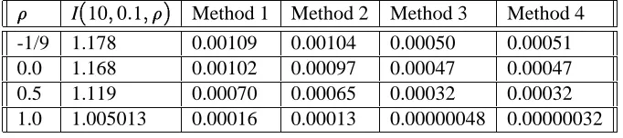
Table 2 shows the standards errors, again in dimension n=10, using =0:1. This represents a volatility of10percent per year for each of the underlying assets prices.
I(10;1:0;) Method 1 Method 2 Method 3 Method 4 -1/9 5.91 0.0734 0.0421 0.0423 0.0260 0.0 5.62 0.0697 0.0311 0.0424 0.0204 0.5 4.18 0.0534 0.0219 0.0287 0.0125 1.0 1.65 0.0265 0.0213 0.0083 0.0054
Table 1: Standard errors in dimension n=10for =100%
I(10;0:1;) Method 1 Method 2 Method 3 Method 4 -1/9 1.178 0.00109 0.00104 0.00050 0.00051 0.0 1.168 0.00102 0.00097 0.00047 0.00047 0.5 1.119 0.00070 0.00065 0.00032 0.00032 1.0 1.005013 0.00016 0.00013 0.00000048 0.00000032
Table 2: Standard errors in dimension n=10for =10%
For lower volatilities ( = 10%), the additive importance sampler performs poorly. The method of quadratic resampling yields an error reduction factor ranging from 2 for problems with low correlation to several hundreds for problems with high correlation. Indeed, the cash-flow function is closer to its second order Taylor expansion for lower volatilities. Since quadratic resampling yields exact results for functions that are equal to their second order Taylor expansion, it is likely to give more accurate results for problems with low volatilities.
All calculations were performed on a DECstation 5000 model 200 desktop workstation, using a MIPS R3000 microprocessor at a clock rate of 25 Mhz. All calculations were performed in double precision floating point arithmetics. The simulation program was written in the
C programming language, and compiled without any optimization. The resulting computing
times for each run of 4000 samples were just below 1 second.
Tables 3 and 4 present the same results in dimension n = 5. The conclusions are similar. For high volatilities, quadratic resampling reduces the error by a factor ranging from 2 (low correlation) to 5 (high correlation). When combined with additive importance sampling, the total error reduction factor ranges from 5 to 10, corresponding to a reduction factor in computing time ranging from 25 to 100. For lower volatilities, the additive importance sampler performs again poorly. The method of quadratic resampling yields an error reduction factor ranging from 5 for problems with low correlation to several hundreds for problems with high correlation. In Table 4, the error reduction of Method 4 over Method 1 ranges from 5 to 1000, corresponding to a reduction factor in computing time ranging from 25 to 1 million. The resulting computing times for each run of 4000 samples were about 1/3 of a second.
I(5;1:0;) Method 1 Method 2 Method 3 Method 4 -1/4 4.39 0.0719 0.0365 0.0230 0.0141 0.0 4.07 0.0594 0.0186 0.0255 0.0088 0.5 3.29 0.0448 0.0102 0.0205 0.0058 1.0 1.65 0.0284 0.0183 0.0067 0.0028
Table 3: Standard errors for n=5and =100%
I(5;0:1;) Method 1 Method 2 Method 3 Method 4 -1/4 1.141 0.00133 0.00126 0.00027 0.00027 0.0 1.126 0.00117 0.00110 0.00024 0.00024 0.5 1.090 0.00079 0.00073 0.00017 0.00016 1.0 1.005013 0.00017 0.00011 0.00000040 0.00000017
Table 4: Standard errors for n=5and=10%
I(100;1:0;) Method 1 Method 2 Method 3 Method 4 0.0 13.58 0.1235 0.0984 0.0994 0.0818
0.5 7.94 0.0850 0.0694 0.0486 0.0422
[image:33.612.116.451.243.316.2]1.0 1.65 0.0301 0.0294 0.0087 0.0084
Table 5: Standard errors for n=100and=100%
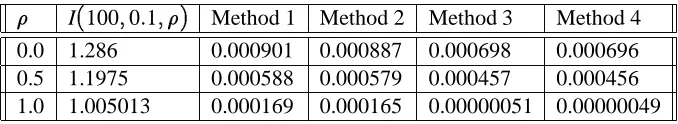
I(100;0:1;) Method 1 Method 2 Method 3 Method 4 0.0 1.286 0.000901 0.000887 0.000698 0.000696 0.5 1.1975 0.000588 0.000579 0.000457 0.000456 1.0 1.005013 0.000169 0.000165 0.00000051 0.00000049
[image:33.612.114.453.543.605.2]reduction factor ranges from 1.5 to 3.6, corresponding to a reduction factor in computing time ranging from 2.3 to 13. For lower volatilities, the additive importance sampler performs again poorly. The method of quadratic resampling yields an error reduction factor ranging from 1.3 for problems with low correlation to several hundreds for problems with high correlation. In Table 6, the error reduction of Method 4 over Method 1 ranges from 1.3 to 350, corresponding to a reduction factor in computing time ranging from 1.7 to 100,000.
The resulting computing times for each run of 4000 samples were about 1 minute and 10 seconds. In general, the computation time is quadratic in the dimension n, since the computation of each sample requires to compute the transformation X=VZ, and V is a nn matrix.
To illustrate typical computing time in practical cases, let us consider the computation of
I(10;1:0;0:0)using Method 4. The result, presented in Table 1, is5:62, and has a standard error of approximately0:02. Using the central limit theorem, we see that the accuracy for a confidence level of99:995% is approximately 0:08(4 times the standard error). In order to make the last digit significant, an accuracy of0:01(8 times higher) is required. Hence, the computation time for 0:01 accuracy would be 88 = 64 times higher. The result would be obtained in about 1 minute of computation on the same hardware platform, with 256000samples. With Method 1, the same result would be obtained in about 12 minutes of computation, using more than 2.5 millions of samples. Not surprisingly, Table 2 shows that problems with lower volatility require much less computing time. Even for low correlations, three digit accuracy is achieved in a small fraction of a second, and four digit accuracy in a couple of seconds (the error margin of Method 3 for=0:0is about40:000470:002for a confidence level of99:995% using only 4000 samples, i.e. a computation time of 1 second).
In general, the computing time may vary from several minutes to a fraction of a second, depending of the characteristics of the covariance matrix, and on the accuracy required. Since the accuracy of Monte Carlo methods is proportional to the square root of the number of samples, getting one additional significant digit requires a computing time 100 times longer on a given hardware platform.
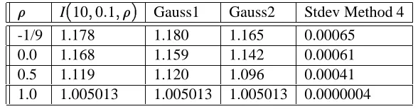
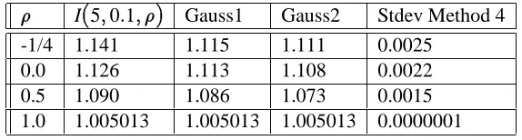
6.2 Comparison with classical Gaussian rules
We implemented several classical Gaussian integration rules proposed in [Stroud, 71] and experimented with them on the above test case.
We present below some results for 2 different rules, designed for approximating integrals of the form:
I(f)= Z
Rnf
(z1;. . .;zn) exp(
P
n
k=1z
2
k=2)
p 2
n dz1. . . dzn
Gauss1 is a classical Cartesian product rule of the form described in Section 4.2. It is exact if
f is a polynomial of degree 3.
In dimension 1, the three sample points are p
3,0, and p