ADAPTIVE COLOR FILTER ARRAY INTERPOLATION ALGORITHM BASED ON HUE TRANSITION AND EDGE DIRECTION

A NEW HYBRID APPROACH FOR PREDICTION OF MOVING

VEHICLE LOCATION USING PARTICLE SWARM

OPTIMIZATION AND NEURAL NETWORK

1_{BABY ANITHA, E. AND} 2_{DR.K.DURAISWAMY}

1_{Assist.Prof.,Department of CSE , K.S.R College of Engineering} 2_{Dean(academic), Department of CSE, K.S. Rangasamy College of Technology}

Tiruchengode, Namakkal District, Tamilnadu, India. E-mail: [email protected], [email protected].

ABSTRACT

The modeling of moving objects can attract the lots of research interests. The moving objects have been developed as a specific research area of Geographic Information Systems (GIS). The Vehicle movement location prediction based on their spatial and temporal mining is an important task in many applications. Several types of technique have been used for performing the vehicle movement prediction process. In such a works, there is a lack of analysis in predicting the vehicles location in current as well as in future. Accordingly we present an algorithm previously for finding optimal path in moving vehicle using Genetic Algorithm (GA). In the previous technique there is no complete assurance that a genetic algorithm will find an optimum path. This method also still now needs improvement for optimal path selection due to fitness function restricted to prediction of complex path. To avoid this problem, in this paper a new moving vehicle location prediction algorithm is proposed. The proposed algorithm mainly comprises two techniques namely, Particle Swarm optimization Algorithm (PSO) and Feed Forward Back Propagation Neural Network (FFBNN). In this proposed technique, the vehicles frequent paths are collected by watching all the vehicles movement in a specific time period. Among the frequent paths, the vehicles optimal paths are calculated by the PSO algorithm. The selected optimal paths for each vehicle are used to train the FFBNN. The well trained FFBNN is then utilized to find the vehicle movement from the current location. By combining the PSO and FFBNN, the vehicles location is predicted more efficiently. The implementation result shows the strength of the proposed algorithm in predicting the vehicle’s future location from the current location. The performance of the new algorithm is evaluated by comparing the result with the GA and FFBNN. The comparison result demonstrates the proposed technique acquires more accurate vehicle location prediction ratio than the GA with FFBNN prediction ratio, in terms of accuracy.

Keyword

s:

Moving Vehicle Location Prediction, Particle Swarm Optimization Algorithm Feed Forward Back Propagation Neural Network, Frequent Paths, Genetic Algorithm, Optimal path.

1. INTRODUCTION

Data mining and knowledge discovery became more popular in the research field. Data mining is defined as discovery of interesting, implicit knowledge, and previously unknown data from large dataset. Spatial data mining is one of the requirements of data mining process spatial data. Spatial data mining is the process of extraction of implicit information, economical, social and scientific problems, spatial relations, or other patterns not explicitly stored in spatial databases [5]. There is an increasing interest in spatial data

specific type of moving objects [7]. The modeling of moving objects can attract the lots of research interests. The moving objects have been developed as a specific research area of Geographic Information Systems (GIS). Several types of models and algorithms have been proposed to hold the continuously changing positions of moving objects. There are mainly two different perspectives when dealing with moving objects databases .First one is the location management perspective and the second one is the spatio-temporal data perspective. A moving object can be defined as an object that changes its geographical position. Such object integrates spatial and temporal characteristics [9]. In sensor and mobile computing technology, enormous amounts of data about moving objects are being collected for tracking of mobile objects, whether it is a small cell phone or a giant ocean liner is accessible with embedded GPS devices and other sensors. Such enormous amount of data on moving objects poses great challenges one for analysis of such data and exploration of its applications [10]. Trajectory data are ubiquitous in the real world. Currently growth in RFID, video, satellite, sensor, and wireless technologies has made it possible to scientifically track object movements and collect huge amounts of trajectory data, e.g., animal movement data, vessel positioning data, and hurricane tracking data[11]. In Swarm Intelligence based algorithms are attracting more researchers. These algorithms more robustness and flexibility for those problems under dynamic atmosphere. Particle swarm optimization (PSO) is one of the popular swarm intelligence based methods [22]. In this paper, we propose a moving vehicle location prediction algorithm which is to predict the vehicle’s future location from the current location. By combining the proposed algorithm with particle swarm optimization (PSO) and Feed Forward Back propagation Neural Network (FFBNN), the vehicle’s location is predicted effectively. The PSO based algorithm is to adaptively identify the optimal path in a dynamic environment. The optimal paths are then used to train the FFBNN. The well trained FFBNN are used to predict the vehicle’s future location from the current location.

The remaining of this paper is structured as follows. Section two briefly reviews the related work in prediction of moving object. Section three discusses the proposed algorithm, which is detailed in its subsection. Experimental results are shown in section four; The Section five concludes the paper.

2. RELATED WORKS

In the literature works deals about the moving objects or moving vehicles location prediction techniques.

Ivana Nizetic et al. [12] have discussed a conceptual model for predicting moving object’s future locations can be very useful in many application areas and data model of moving objects considering various object’s characteristics. The location of the vehicle equipped with a GPS device can be received almost continually. The proposed approach has a great issue to predict moving object’s next position.

Jorge Huere Pena et al. [13] has proposed technique to store data about moving objects. For the analysis of movement data an overview of the existing data mining techniques and some future guidelines are also presented. The proposed approach also summarized the main developments in systems or prototypes like Hermes, SECONDO, Move Mine and Swarm.

Jidong Chen et al. [15] first proposed model for the road network and moving objects in a graph of cellular automata, which makes full use of the constraints of the network and the stochastic behavior of the traffic. The combined model to predict the future trajectories of moving objects.

Gyozo Gidofalvi et al. [16] have developed a novel approach for continuously streaming moving object trajectories for traffic prediction and management. The proposed methods, data structures, and a prototype implementation in a DSMS for managing, mining, and predicting the incrementally evolving trajectories of moving objects in road networks. The approach can be measured on a large real-world data set of moving object trajectories, starting from a fleet of taxis and frequent routes can be efficiently discovered and used for prediction.

utilizing technologies such as Global Positioning System (GPS), Global System for Mobile Communications (GSM) etc.,.

Ajaya Kumar Akasapu et al. [17] have proposed a model for analyzing the trajectories of moving vehicles and develop the algorithm for mining the frequency patterns of Trajectory data .The trajectory data are normally obtained from location-aware devices that capture the position of an object at a specific time interval.

Ying-yuan Xiao1et al. [20] introduced a location prediction model of moving objects with uncertain movement patterns based on grey theory. The presented location prediction model is applied to predict the future location of uncertain moving objects. The proposed model Comparing with linear prediction model, these location prediction models not only relaxes the limitation to motion pattern of moving objects and the requirement for accuracy of sampling data, but also improve accuracy clearly.

Rohayanti Hassan et al. [18] has proposed path optimization algorithm to determine the efficient optimal route tours in Virtual Environment. These optimal route tours mainly based on three criteria. 1. Shortest distance, 2. Crowd avoidance and 3. Small scale search area. Prim’s algorithm is applied in order to generate the optimal path. The experimental result shows that algorithm capable to minimize travel cost although maximize the visiting place in virtual environments.

Anthony J.T. Lee et al. [21] has drawn a graph-based mining (GBM) algorithm for mining the frequent trajectory patterns in a spatial–temporal database. The algorithm consists of two phases. The first phase, transform all trajectories in the database into a mapping graph. And second phase, a TI-list for each vertex to record all trajectories that pass through the vertex using the information recorded in TI-lists created, the proposed algorithm using depth-first search manner to mine all frequent

trajectory patterns. The experimental results

illustrate that the GBM algorithm outperforms the Apriori-based and Prefix-Span-based algorithms by more than one order of magnitude. Whereas the GBM algorithm can mine frequent trajectory patterns efficiently, there are still some issues to be addressed in future research.

Yanfang Deng [4] proposed PSO algorithm with priority based encoding scheme based on a fluid neural network (FNN) to search shortest path in traffic network. This algorithm overcomes the weight coefficient symmetry restriction of FNN.

In many applications, the moving vehicles location prediction plays an important task. A lot of methods were developed to find the vehicle location. In our previous work we proposed heuristic moving vehicle location prediction algorithm. Prediction of the vehicle’s future location by finding a vehicle optimal path is determined by one of the optimization techniques called genetic algorithm (GA). The selected optimal paths for each vehicle are used to train the FFBNN. The trained FFBNN is then used to determine the vehicle’s future location from the current location [23] [24].

There is no complete assurance that a genetic algorithm will find an optimum path. This method also still now needs improvement for optimal path selection due to the fitness function restricted to prediction of complex path.

The above mentioned in the literary works are resolvable, after that the moving vehicle’s location prediction performance is improved with higher accuracy.

3. MOVING VEHICLE’S LOCATION PREDICTION

The proposed Moving Vehicle’s Location prediction technique consists of four phases, frequent path selection, optimal path prediction using PSO, optimal path training in FFBNN, and vehicle’s future location prediction by FFBNN. This proposed method predicts the vehicle’s location by finding the vehicles frequent paths and allocating weights to each of the nodes (junctions). Each path’s frequent values and node’s weight values are utilized to find the vehicle’s optimal paths via the optimization algorithm for PSO. The optimal paths from the PSO are then utilized in the FFBNN training and testing process. The steps of proposed technique is as followed,

Step Description

1. Vehicle visiting paths in different time Periods are collected.

2. Frequent paths for each vehicle are computed

3.

After that, the frequent paths are given to the PSO optimization process to choose optimal paths for each vehicle 4. The Optimal path is trained by FFBNN.

3.1 Frequent path selection using a graph

In this method, to construct an undirected graph G and Locations are considered as nodes (or) junctions. Edges connecting the nodes denote as a path p. The number of vehicles in the designed graph is represented as v= (v1, v2, v3… vc), where c

is value for number of vehicles and the paths are represented as p= (p1, p2, p3…..pz). The weight wn

is assigned to the nodes with random values [1, w]. The vehicle visited path is collected in various time period T= (t1, t2….tp).The undirected graph is

[image:4.612.143.234.285.348.2]

shown in Figure. 1

Figure 1: Construction of Graph

Node n= (node1, node2, node3, node4, node5) Vehicles V= (v1, v2, v3, v4, v5)

Number of available Paths P=7

The vehicle v1 initially traverse at the node 1 in a

time period t1 and it’s next to visit the node 2 by

using the path 1->2 and then it visit the nodes 3 and node 4 via the paths 2->3 and 3->4 respectively. In same the time period t1 the other vehicles traversing

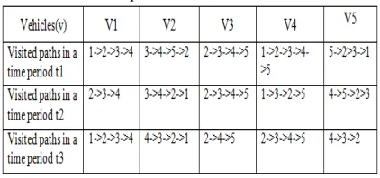
[image:4.612.90.301.548.647.2]

paths are also to be calculated. The same process is repeated for all vehicles in different time periods. In Table 1 list out the collected paths from the above mentioned graph in three time periods.

Table 1: Frequent Path in Three Time Periods

In Table 1, the vehicles are using different paths to reach at the same target node in different time periods. Likewise in different time periods, the vehicles vc visited paths are collected and the

frequency value of path visited more than once by the particular vehicle vc is calculated. Based on the

frequency value, the vehicle vc frequently visited

paths p is computed and an index value is allocated for each computed frequent path. The number of frequent paths for the vehicle vc is denoted as

fpvc= (p1, p2, pj) and the corresponding index value

for the frequent path is represented as

I vc = (i1, i2…..ix) where x is a value for number of

frequent paths selection in the vehicle vc.

3.2 Particle Swarm Optimization (PSO)

PSO is a stochastic optimization technique inspired by social behavior of bird flocking or fish schooling. It was developed by Jim Kennedy (social psychologist), Bureau of Labor Statistics and Russ Eberhart (electrical engineer), Purdue University. A concept for optimizing nonlinear functions using particle swarm methodology [1]. PSO has been used by many applications of several problems. Such as image retrieval, human movement bio mechanism optimization, cancer classification, gene clustering, object tracking etc., PSO is a population based search approach that determines the optimal solution utilizing a set of flying particle with velocities that are dynamically adjusted according to performance as well as neighbors in the search space [2].

Each single solution is a bird called as a particle in the search space. The entire particles have fitness values which are evaluated using fitness function and have velocities which direct the flying of the particles. In all iteration, every particle is updated by two best values. First, pbest which is the best solution achieved so far by that particle. Second, gbest which is the best value obtained so far by any particle in the population. PSO can accelerate each particle toward its previous best position, and global best position locations, with a random weighted acceleration at each time [3].

3.3 Optimal Path Prediction Using PSO

In Particle swarm optimization to establish the optimal path for all vehicles from the number of frequent paths fp. The selected optimal path for each vehicle is utilized to identify the vehicle future location. The PSO method initialized with population of N individuals and particle i are generated randomly that is represented as Xi = (xi1,

xi2, xi3…... xin), and each particle position is denoted

as index ix. The best previous position of particle i

represented as Pi = (pi1, pi2…. Pin), The particle

velocity is represented as Vi= (vi1, vi2….. vin) .Now

) * 1 ( ) (

n w n w f

p v x i

f = + ₋

xmax ] is the range of position. Particle updates their

velocity and positions based on two best values. First one is the Personal best, which is the location of its highest fitness value. Second is the Global best which is the location of overall best value (fitness) and it can be obtained by any particle.

3.3.1 Fitness Function

At this stage, the randomly generated particles are evaluated by the fitness function. The Fitness function is applied to each particle to find the best value. The corresponding path’s frequency and node’s weight values of particles index values are utilized in the fitness function calculation. The fitness function is

(1)

(2)

Where, Fvc _{is the fitness function of the i}th particle generated in the vehicle vc, and

f

i

x

is the

individual fitness value of the index

i

_x. In equation (2),

v (p

f

)

is the frequency value of the frequent

path

p

f

,

which is presented in the index

i

xand

n

n

w

w

₋₁

&

are the weight value of the nodes, and

the path pf is presented between these two nodes.

The individual particle best fitness value is calculated by equation (2) and set of particle fitness function is also calculated using equation (1). Then, the fitness value is calculated for all the particles and overall best value (fitness) is also calculated for the particles that have the highest fitness value are selected. In all iteration, particle updates their positions and velocity according to equations. Among the best value particle, some particle contains same index values. This duplication of index values creates difficulty in the further process. So, the repeated index values are taken at one time and the remaining repeated values are eliminated.

V

in

= w*v

in

+c

1

* r

1

* (p

bn

- x

in

) + c

2

* r

2

*

(p

gn

- x

kn

) (3)

x

in

= x

in

+ v

in

(4)

Where, Vin is the current speed (velocity) of

particle i in the n dimensions, xin is the current

position of ith particle is the inertia weight in the range of [0-1], c1 and c2 are the accelerate

parameters and currently set to 2.0 respectively, r1

and r2 is the random number between [0, 1], pbn and

pgn are the corresponding personal best and global

best. In equ (4) can update the location of new particle.

The inertia weight w is to control the force of the particle by considering the contribution of the previous velocity. It’s basically controlling how much memory of the previous flight direction will influence the new velocity. A similar change is made from the PSO. If w > 1, then the velocity will reduce the time, the particle will increase speed to maximum velocity and the swarm will be divergent. If w < 1, then the velocity of particle will decrease until it reaches zero.

(5)

Where, wmax and wmin is the initial and final weight, itermax is the maximum iteration number, iter is the recent iteration number. In equation (5), diversification attributes is gradually decreased and a certain velocity and moves the current position close to pbest and gbest can be calculated [14].

3.3.2 PSO algorithm

Step 1: Initialize position and velocity of all

particles (vehicle) randomly generated in the N Dimensional space.

Step 2: For each particle (vehicle) evaluates the

fitness function and update the global optimum position.

Step 3: Compare particles fitness value with the

pbest. If current value is better than pbest then Rest pbest value equal to the current value and pbest location equal to current location in N-dimensional.

Step 4: Compare fitness evaluation with particles

overall pbest. If current value is better than gbest, then reset gbest to current particles array index and value.

Step 5: Update particle velocity and position using

equation (3), (4) respectively.

Step 6: Repeat 2 to 5 until step criterion is met;

maximum number of iterations is computed.

3.4 To Train the Optimal Path Using FFBNN

For above process, we have number of optimal path index values for each vehicle and these optimal ∑

= =

X

x x i f x vc

F

paths are used to obtain the vehicle future location by FFBNN. To achieve the location prediction process, the optimal path index values are selected by the vehicle’s best (fitness) value and given to the FFBNN. The Feed Forward Back Propagation Neural Network (FFBNN) is hired to perform the training and testing process. On training stage, each index value of vehicle’s best particle value and the corresponding path’s nodes are given as input to the FFBNN. For example, select one index value

i

_x from the best particle vehicle vc. Now, we have

[image:6.612.98.302.381.511.2]

taken the FFBNN input as

i

_xindex corresponding path node values n1andn2. In FFBNN, there is

H

_d number of hidden layers and one output layer, which is an individual fitness value of the index

i

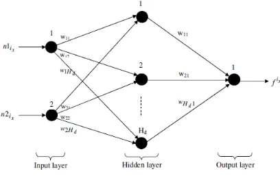
_x as_f i_x. The FFBNN is well trained by this optimal path and provided an accurate fitness value for the input node values. The proposed vehicle future location prediction FFBNN structure is shown in Figure. 2.

Figure 2: Construction of Optimal Paths Training In FFBNN

In Figure 2 contains two input units, one output unit, and Nd _{hidden units. At first, the input data} are transmitted to the hidden layer and then, to the output layer. This progression is called the forward pass of the back propagation algorithm. Every node in the hidden layer gets input from the input layer and then multiplexed with appropriate weights and summed. The hidden layer input value calculation function is said to be bias function.

) 2 1

1(whn i_xh whn i_xh d

H

h x

i

Y ∑ +

= + = β

(6)

In Equation (6), n1ix and n 2ix are the input node values of the index

x

i . The output of the

hidden node is the nonlinear transformation of the resulting sum. The same process is followed in the output layer. The following equation (7) denotes the activation function of the output layer. The output values from the output layer are compared with target values and the learning error rate for the neural network is computed, which is given in equation (8). (7) (8) In equation (8),

γ

is the learning error rate of the

FFBNN, ix h

D is the desired output, and ix h f is

the actual output. The error between the nodes is transmitted back to the hidden layer and this process is called the backward pass of the back propagation algorithm. The reduction of error by back propagation algorithm is described in the subsequent steps.

Step 1: At first, the weights are allocated to the

hidden layer. The input layer can hold a constant weight, whereas the weights for output layer are selected at random. After that the bias function and output layer activation function are calculated by using the equation. (6) and (7).

Step 2: Next, the back propagation error is

computed for each node and then weights are updated by using the equation (9).

(9) Where, the weight∆ wixh _{is changed, which is}

given as,

(10)

Where,

φ

is the learning rate that usally ranges from 0.2 to 0.5, and

E

(ε) is the Back propagation error. The bias function, activation function, and back propagation error calculation process are continued till the back propagation error gets

x i c v p y e − + = 1 1

α

∑

− =

−

=

1 0

1

d x x i H h i h h d

f

D

H

γ

h x i w h x i w h x i

w = + ∆

reduced i.e. (ε)

<

0

.

1

E

. If the back propagation error reaches a minimum value, then the FFBNN is well trained by the path node values for performing the vehicle location prediction. The well trained FFBNN provide a proper fitness value for the respective input path values.

3.5 Vehicle Future Location Prediction in FFBNN

The well trained FFBNN is used to predict the vehicle’s future location. Let us assume that the vehicle vc initial starting node

n

i is given by the

user. After, all the possible paths

p

via nodes visited by the vehicle vc is given to the well trained

FFBNN and we got the fitness values for all the input paths

p

. Among the paths, the vehicle vc visiting next path is predicted by their fitness value output from the FFBNN, which are given as,

} , 2 , 1 max{

z p f p f p f c

v

F = L

(11)

In Equation (11),

z p

f _{is the fitness value of}

the path p_{z and} c v

F _{have the path value, which has}

the higher fitness value than the others. Suppose we get the path

p

_z having a highest fitness value than the other paths, and then this highest fitness value path is considered as a next visiting path of a vehicle

v

_cfrom the current node

n

i. In this way, the

vehicle’s future location is predicted from the current position. The well trained FFBNN reduces the time complexity as well as giving the optimal future vehicles’ paths, because the training process in FFBNN is carried out by the Particle swarm algorithm. The similar procedure is used for all vehicles to predict the future location efficiently.

4.EXPERIMENTALRESULT

In our implementation we use MATLAB version 7.12. The proposed technique accurately finds the moving vehicle’s location by finding their frequent paths. Here, all the vehicles frequent moving paths are collected and then optimal frequent paths of each vehicle are computed by Particle swarm optimization technique and each vehicle frequent path is trained in the FFBNN and afterward in performance testing, the vehicles moving location is

[image:7.612.323.511.147.240.2]

predicted. Five vehicles frequent moving paths are composed at a certain time period, which is listed in the below table 2.

Table 2: Sample Frequent Paths of Five Vehicles

Vehicles A B C D E

Frequent

Paths

1-3 1-8 5-10 6-10 5-9

3-5 2-10 7-9 7-9 3-5

2-9 4-8 6-9 10-5 2-8

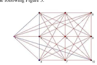
The Table 2 shows the vehicles moving paths with different starting nodes. These paths are not the most frequent path of the vehicles. Therefore we have to find most frequent paths for each vehicle. By using these frequent paths, the optimal frequent paths are computed and given to the FFBNN. The sample moving paths of vehicle A is illustrated in

the following Figure 3.

Figure 3: Sample Moving Paths of Vehicle A (10-4)

[image:7.612.319.507.384.511.2]

Table 3: Optimal Frequent Paths discovered for Each Vehicle by PSO and FFBNN

Vehicles Optimal Frequent Paths

A 10 9 4 10 4 2 5 6 3 2

B 1 9 7 5 2 3 7 4 9 3

C 1 8 1 5 3 6 2 4 9 8

D 3 2 5 4 5 4 8 3 6 4

E 10 1 3 9 4 6 7 5 4 2

The proposed technique’s prediction accuracy is shown in the below Table 4. The vehicle prediction accuracy is calculated by utilizing the formula,

(12)

AC - Accuracy

Cp - Correctly predicted paths

[image:8.612.323.518.166.290.2]

Np - Total number of optimal frequent paths

Table 4: Different Vehicles Performance Accuracy Results by PSO and FFBNN

Vehicles A B C D E

Accuracy 80 85 75 100 90

Also in previous technique, the optimal frequent paths are computed by using Genetic Algorithm (GA). These frequent paths are given to the FFBNN for performing the training process and the trained FFBNN is tested with moving vehicles. The five vehicles predicted paths by FFBNN is given in the below Table 5. Moreover, the prediction accuracy of FFBNN for five vehicles is given in Table 6.

Table 5: Optimal Frequent Paths discovered for Each Vehicle by GA and FFBNN

Vehicles Optimal Frequent Paths

A 3 2 4 6 1 2 3 2 5 10

B 1 9 5 10 7 1 6 4 2 8

C 6 9 6 1 7 10 10 8 4 6

D 7 2 8 5 9 3 1 6 4 10

E 7 6 6 10 5 3 8 5 2 4

Table 6: Different Vehicles Performance Accuracy Results by FFBNN and GA

Vehicles A B C D E

Accuracy 60 85 40 95 60

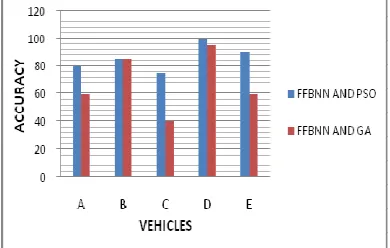
The comparison result of both methods performance measures are given in the Figure 4.

Figure 4: Prediction Accuracy for Proposed and Existing Methods Using Graph.

As can be seen from Tables 4, 6 and Figure 4, the proposed technique has offered 95% mean accuracy but the previous work technique has given only 88% accuracy. Here all five vehicles prediction accuracy results are higher than the previously used method and the prediction accuracy of vehicle B is same for both methods. The graphical representation of the accuracy performance results shows that moving vehicle location prediction technique more accurately determines the future moving location than previous work method.

5.CONCLUSION

[image:8.612.98.291.383.420.2]

REFERENCES:

[1] R. C. Eberhart and Y. Shi, “Particle Swarm Optimization, Developments, Applications, And Resources,” in Proc. Congress on Evolutionary Computation 2001 IEE service center, Piscataway, NJ. Seoul, Korea. 2001.

[2] Koffka Khan , Ashok Sahai, “A Comparison ofBA, GA, PSO, BP and LM for Training Feed forward Neural Networks in e-Learning Context” I.J. Intelligent Systems and Applications,Vol. 7,2012, pp . 23-29. [3] S. Geetha, G. Poonthalir and P. T. Vanathi,

“A Hybrid Particle Swarm Optimization with Genetic Operators for Vehicle Routing Problem“ Journal of Advances in Information Technology, Vol. 1,2010, pp. 4. [4] Yanfang Deng, Hengqing Tong, “Dynamic Shortest Path Algorithm in Stochastic Traffic Networks Using PSO Based on Fluid Neural Network”, Journal of Intelligent Learning Systems and Applications, Vol. 3, 2011 pp.11-16.

[5] Deren Li and Shuliang Wang, “Concepts, Principles and Applications of Spatial Data Mining and Knowledge Discovery”, In Proceedings of International Symposium on Spatio-temporal Modeling, Beijing, China, 2005 pp. 1-13.

[6] Diansheng Guo and Jeremy Mennis, “Spatial data mining and geographic knowledge discovery-An introduction”, Computers, Environment and Urban Systems, Vol. 33, 2009 pp. 403-408. [7] Sotiris Brakatsoulas, Dieter Pfoser and

Nectaria Tryfona, “Modeling, Storing and Mining Moving Object Databases”, In Proceedings of the International Conference on Database Engineering and Applications Symposium, 2004, pp. 68 - 77. [8] D.Malerba11, “Mining Spatial Data:

Opportunities and Challenges of a Relational Approach” IASC 07, 2007. [9] Martin Ester, Hans-Peter Kriegel and Jorg

Sander, “Algorithms and Applications for Spatial Data Mining”, Geographic Data Mining and Knowledge Discovery, Research Monographs in GIS, 2001, pp. 160-187.

[10] Xiaolei Li, Jiawei Han and Sangkyum Kim, “Motion-Alert: Automatic Anomaly Detection in Massive Moving Objects”, In

Proceedings of IEEE international conference on intelligence and security informatics, San Diego, Calif, Vol. 3975, 2006, pp.166-177.

[11] JaeGil Lee, Jiawei Han, Xiaolei Li and Hector Gonzalez, “TraClass: Trajectory Classification Using Hierarchical RegionBased and TrajectoryBased Clustering”, In Proceedings of International Conference on Very Large Data Base, Auckland, New Zealand, 2008.

[12] Ivana Nizetic and Kresimir Fertalj, “Automation of the Moving Objects Movement Prediction Process Independent of the Application Area”, Computer. Sci. Inf. Vol. 7, Issue 4, 2010.

[13] Jorge Huere Pena and Maribel Yasmina Santos, “Representing, Storing and Mining Moving Objects Data”, In Proceedings of the World Congress on Engineering, London, U.K, Vol. 3,2011, pp. 6 - 8.

[14] K. Premalatha and A.M. Natarajan, “Hybrid PSO and GA for Global Maximization” Int. J. Open Problems Compt. Math., Vol. 2, 2009 pp. 4, 2009.

[15] Jidong Chen, Xiaofeng Meng, Yanyan Guo, St, Hui Sun, “Modeling and Predicting Future Trajectories of Moving Objects in a Constrained Network”, In Proceedings of International Conference on mobile data management, 2006, pp. 156.

[16] Gyozo Gidofalvi, Christian Borgelt Manohar Kaul, “Frequent Route Based Continuous Moving Object Location- and Density Prediction on Road Networks” , In Proceedings of the 19th ACM SIGSPATIAL International Conference on Advances in Geographic Information Systems, 2011, pp 381-384.

[17] Ajaya Kumar Akasapu, Lokesh Kumar Sharma, G.Ramakrishna, “Efficient Trajectory Pattern Mining for both sparse and Dense Dataset”, International Journal of Computer Applications Volume 9, 2010, pp.5.

[19] Thi Hong Nhan Vu, Jun Wook Lee, and Keun Ho Ryu, “Spatiotemporal Pattern Mining Technique for Location-Based Service System”, ETRI Journal, Volume 30, 2008, pp. 3.

[20] Ying-yuan Xiao, Hua Zhang, Hong-ya, Wangand Fa-yu Wang, “Location Prediction of Moving Objects with Uncertain Motion Patterns” Complex Systems and Applications—Modeling, Control and Simulations,2007, pp. 503-507.

[21] Anthony J.T.Lee,Yi-An Chen,Weng-Chong Ip, “Mining frequent trajectory patterns in spatial–temporal databases” Information Science,Vol 179,2009,pp.2218-2231. [22] Hazem Ahmed, Janice Glasgow, “Swarm

Intelligence: Concepts, Models and Applications” Technical Report 2012-585. [23] E.Baby Anitha, Dr.K.Duraiswamy,

“Prediction Of Vehicle Movement Using Spatial Mining: A Recent Survey” International Journal of Advanced Research in Technology, Vol. 2 Issue 4, 2012. [24] E.Baby Anitha, Dr.K.Duraiswamy, “A