Exponentiated Gumbel Model for Software Reliability
Data Analysis using MCMC Simulation Method
Raj Kumar
National Institute of Electronics and Information Technology,
Gorakhpur, U.P., India
Ashwini Kumar Srivastava
Dept. of Computer Application, Shivharsh.Kisan P.G. College,Basti, U.P., India
Vijay Kumar
Dept. of Maths & Statistics, D.D.U. Gorakhpur University,Gorakhpur, U.P., India
ABSTRACT
In this paper, the Markov chain Monte Carlo (MCMC) method has been used to estimate the parameters of Exponentiated Gumbel(EG) model based on a complete sample. A procedure is developed to obtain Bayes estimates of the parameters of the Exponentiated Gumbel model using MCMC simulation method in OpenBUGS, an established software for Bayesian analysis using Markov Chain Monte Carlo (MCMC) method. The MCMC methods have been shown to be easy to implement computationally, the estimates always exist and are statistically consistent, and their probability intervals are convenient to construct. The R functions are developed to study the statistical properties, model validation and comparison tools of the proposed model and the output analysis of MCMC samples generated from OpenBUGS. The proposed methodology is suitable for empirical modeling. A simulated data set is considered for illustration under uniform and gamma sets of priors.
Keywords
Exponentiated Gumbel(EG) model, Parameter estimation, Maximum likelihood estimate (MLE), Bayes estimates, Markov Chain Monte Carlo (MCMC), OpenBUGS.
1.
INTRODUCTION
The Exponentiated Gumbel (EG) model has been proposed as a modification of the classical Gumbel model[1]. Since the Gumbel model[2] yields narrower confidence intervals than the some other extreme value models but has also the risk of under-estimating the certain important characteristic of the model. Hence, the choice of model is not trivial.
Recently, Nadarajah in 2006[3,4] introduced the Exponentiated Gumbel (EG) model as
F(x; , ) exp exp u ; ( , ) 0, x .
Where u= -(x/σ), Moreover, hazard-rate functions, moments, asymptotics and maximum likelihood functions were presented.
In this paper, we have proposed the EG model for modeling the software reliability data. We have obtained the ML estimates and associated probability intervals. The Bayes estimation of the EG model is considered when both parameters are unknown. It is observed that the Bayes estimates cannot be computed explicitly under the assumption of independent uniform and gamma priors for the parameters. We have developed the procedure to generate MCMC samples using Gibbs sampling technique from the posterior density function in OpenBUGS, Based on the generated posterior samples, we can compute the Bayes estimates of the unknown parameters and also can construct highest posterior
density credible intervals. We have also estimated the reliability function.
One real data set has been analyzed to demonstrate how the proposed method can be used in practice for software reliability data.
2.
MODEL ANALYSIS
2.1
Probability density function(pdf)
The probability density function is given by
x x
f (x) exp exp exp ;
where x , 0, 0.
(2.1)
The R functions dexpo.gumbel( ) and pexpo.gumbel( ) given in [5] can be used for the computation of pdf and cdf, respectively. Some of the typical EG density functions for different values of and for σ = 1 are depicted in Figure 1.
It is clear from the above figure that the density function of the Exponentiated Gumbel model can take different shapes
2.2
Cumulative density function(pdf)
The distribution function of Exponentiated Gumbel model with two parameters is given by
x
F(x)exp exp ; x , 0, 0
[image:1.595.331.537.430.607.2] , (2.2)
where, > 0 is the shape and > 0 is the scale parameter. The two-parameter Exponentiated Gumbel model will be denoted by EG(,σ).
2.3
The Reliability function
The reliability/survival function is
x R(x) 1 exp exp .
(2.3)
Here, - < x < , > 0 and > 0. The R function sexpo.gumbel( ) given in [5], computes the reliability function.
2.4
The Hazard function
The hazard rate function is
x x
exp exp exp
h(x; , )
x
1 exp exp
(2.4)
The hazard rate is an increasing function. It has been graphed in Figure 2for scale parameter =1 and different values of shape parameter .
The associated R function hexpo.gumbel( ) given in [5].
2.5
The cumulative hazard function
The cumulative hazard function H(x) defined as
H(x) 1 log F(x) (2.5)
can be obtained with the help of pexpo.gumbel( ) function given in [5] by choosing arguments lower.tail=FALSE and log.p=TRUE. i.e.
-pexpo.gumbel(x,alpha,sigma,lower.tail=FALSE,log.p=TRUE)
2.6
The Failure rate average (fra) and
Conditional survival cumulative hazard
function(crf)
Two other relevant functions useful in reliability analysis are failure rate average (fra) and conditional survival function(crf) The failure rate average of X is given by
x
0
h(x) dx H(x)
FRA(x) =
x x
, x > 0, (2.6)
where H(x) is the cumulative hazard function. An analysis for FRA(x) on x permits to obtain the IFRA and DFRA classes.
The survival function (s.f.) and the conditional survival of X are defined by
R(x)= 1 − F(x)
and
R (x | t) = R (x + t)
R(x) , t > 0, x > 0, R (·) > 0, (2.7)
respectively, where F(·) is the cdf of x. Similarly to h(x) and FRA(x), the distribution of x belongs to the new better than used (NBU), exponential, or new worse than used (NWU) classes, when R (x | t) < R(x), R(t | x) = R(x), or R(x | t) > R(x), respectively.
The R functions hra.expo.gumbel() and crf.expo.gumbel() given in [5] can be used for the computation of failure rate average (fra) and conditional survival function(crf), respectively.
2.7
The Quantile function
The quantile function is given by
q
1
x log log q ; 0 q 1.
(2.8)
The computation of quantiles the R function qexpo.gumbel( ), given in [5] .
2.8
The random deviate generation function
Let U be the uniform (0,1) random variable and F(.) a cdf for
which F-1(.) exists. Then F-1(u) is a draw from distribution F(.) . Therefore, the random deviate can be generated from EG(,σ) by
1
x log log(u) ; 0 u 1.
(2.9) (2.9)
where u has the U(0, 1) distribution. The R function rexpo.gumbel( ), given in [5] , generates the random deviate from EG(,σ).
3.
MLE
(MAXIMUM
LIKELIHOOD
ESTIMATION) AND INFORMATION
MATRIX
For completeness purposes, in this section, we briefly discuss the maximum likelihood estimators (MLE’s) of the two-parameter Exponentiated Gumbel model and discuss their asymptotic properties to obtain approximate confidence intervals based on MLE’s[6].
[image:2.595.60.275.253.495.2]Let x=(x1, . . . , xn) be a random sample of size n from
EG(,σ), then the log-likelihood function L(,σ) can be written as;
n n
i i
i 1 i 1
x x
log L n log n log exp
(3.1)
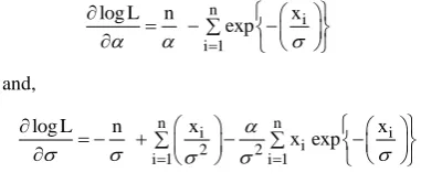
Therefore, to obtain the MLE’s of and σ [7], we can maximize (3.1) directly with respect to and σ or we can solve the following two non-linear equations using Newton-Raphson method
n
i i 1
log L n x
exp and, n n i i i 2 2
i 1 i 1
log L n x x
x exp
3.1
Information Matrix and Asymptotic
Confidence Intervals
Let us denote the parameter vector by
,
and the corresponding MLE of as ˆ
ˆ ˆ,
then the asymptotic normality results in
1
2
ˆ N 0, I( )
(3.2)
where I() is the Fisher’s information matrix given by
2 2
2
2 2
2
ln L ln L
E E
I( )
ln L ln L
E E (3.3)
In practice, it is useless that the MLE has asymptotic variance
1I( ) because we do not know . Hence, we approximate the asymptotic variance by “plugging in” the estimated value of the parameters[8]. The common procedure is to use observed Fisher information matrix O( )ˆ (as an estimate of the information matrix I()) given by
2 2 2 ˆ 2 2 2 ˆ ˆ ( , )
ln L ln L
ˆ
O( ) H( )
ln L ln L
(3.4)
where H is the Hessian matrix,
,
and ˆ
ˆ ˆ,
. The Newton-Raphson algorithm to maximize the likelihood produces the observed information matrix. Therefore, the variance-covariance matrix is given by
1ˆ
ˆ ˆ ˆ
Var( ) cov( , ) H( )
ˆ ˆ ˆ
cov( , ) Var( )
(3.5)
Hence, from the asymptotic normality of MLEs, approximate 100(1-)% confidence intervals for and can be
constructed as
/ 2
ˆ z Var( )ˆ
and ˆ z/ 2 Var( )ˆ (3.3.6)
where z/2 is the upper percentile of standard normal variate.
3.2
Computation of Maximum Likelihood
Estimation
We are using software reliability data set SYS2.DAT - 86 time-between-failures [9] is considered for illustration of the proposed methodology. In this real data set, Time-between-failures is converted to time to Time-between-failures and scaled.
The Exponentiated Gumbel model is used to fit this data set. We have started the iterative procedure by maximizing the log-likelihood function given in (3.1) directly with an initial guess for = 1.15 and = 130.0, for away from the solution. We have used optim( ) function in R with option Newton-Raphson method[10]. The iterative process stopped only after 24 iterations. We obtain ˆ 4.056801, ˆ 151.915039 and the corresponding log-likelihood value = -734.5816. The similar results are obtained using maxLikpackage available in R. An estimate of variance-covariance matrix, using (3.4), is given by
ˆ ˆ ˆ
var( ) cov( , ) 0.1599290 -0.3198579
ˆ ˆ ˆ
cov( , ) var( ) -0.3198579 9.4358089
Thus using (3.5), we can construct the approximate 95% confidence intervals for the parameters of Exponentiated Gumbel model based on MLE’s. Table 1 shows the MLE’s with their standard errors and approximate 95% confidence intervals for and .
4.
MODEL VALIDATION
To study the goodness of fit of the EG model, we compute the Kolmogorov-Smirnov statistics between the empirical distribution function and the fitted distribution function when the parameters are obtained by method of maximum likelihood[11]. For this we have used the R function ks.expo.gumbel( ) given in [5]. The result of K-S test is D= 0.0708 with the corresponding p-value = 0.634. Therefore, the high p-value clearly indicates that EG model can be used to analyze this data set.
[image:3.595.53.244.196.284.2]We plot the empirical distribution function and the fitted distribution function in Figure 3, which indicates reasonable match between the empirical distribution function and the fitted distribution function.
Table 1. Maximum likelihood estimate, standard error and 95% confidence interval
Parameter MLE Std. Error 95% Confidence Interval
alpha 4.056801 0.39632 (3.2800138, 4.8335882)
Therefore, from above result and Figure 3, it is clear that the estimated EG model provides excellent fit to the given data.
The graphical methods widely used for checking whether a fitted model is in agreement with the data are Quantile-Quantile(Q-Q) and Probability-Probability (P-P) plots in model validation. The corresponding R functions are qq.expo.gumbel( ) and pp.expo.gumbel( ) given in [5].
Let ˆF(x) be an estimate of F(x) based on xl, x2,. . . , xn.
The scatter plot of the points
1 1:n
ˆF (p ) versus x
i : n , i = 1 , 2, . . . ,n , is called a
Q-Q plot.
The Q-Q plot shows the estimated versus the observed quantiles. If the model fits the data well, the pattern of points on the Q-Q plot will exhibit a 45-degree straight line. As can be seen from the straight line pattern in Figure 4, the EG model fits the data very well. This is also supported by the Probability-Probability(P-P) plot in Figure 5.
Let xl, x2,. . . , xn be a sample from a given population with
estimated cdf ˆF(x) . The scatter plot of the points
1:n
ˆF(x ) versus pi : n , i = 1 , 2 , . . . , n, is called a P-P plot. If
the model fits the data well, the graph will be close to the 45-degree line[12]. Here we note that all the points in the P-P plot are inside the unit square [0, l] x [0, 1].
As can be seen from Figure 4 and Figure 5 that the data do not deviate dramatically from the line.
5.
BAYESIAN
ESTIMATION
USING
MARKOV CHAIN MONTE CARLO
(MCMC) METHOD
A Monte Carlo method is an algorithm that relies on repeated pseudo-random sampling for computation, and is therefore stochastic (as opposed to deterministic). Monte Carlo methods are often used for simulation. The union of Markov chains and Monte Carlo methods is called MCMC[13]. A Markov chain is a random process with a finite state-space and the Markov property, meaning that the next state depends only on the current state, not on the past[14].
The revival of Bayesian inference since the 1980s is due to MCMC algorithms and increased computing power. The most prevalent MCMC algorithms may be the simplest: random-walk Metropolis and Gibbs sampling. The quality of the marginal samples usually improves with the number of iterations. In Bayesian inference, the target distribution of each Markov chain is usually a marginal posterior distribution, such as each parameter. Each Markov chain begins with an initial value and the algorithm iterates, attempting to maximize the logarithm of the unnormalized joint posterior distribution and eventually arriving at each target distribution. Each iteration is considered a state.
[image:4.595.61.286.74.248.2]The Gibbs algorithm starts by assuming some arbitrarily chosen initial values for the concerned variates and then generating the variate values from the various full conditionals in a cyclic order. That is, every time a variate value is generated from a full conditional, it is influenced by the most recent values of all other conditioning variables and, after each cycle of iteration, it is updated by sampling a new value from its full conditional. The entire generating scheme is repeated unless the generating chain achieves a systematic pattern of convergence. It can be shown that after a large number of iterations the generated variates can be regarded as
Fig 3. The graph of empirical distribution function and fitted distribution function.
[image:4.595.317.538.128.344.2]Fig 5. Probability-Probability(P-P) plot using MLEs as estimate.
[image:4.595.62.273.396.562.2]the random samples from the corresponding posteriors. Readers are referred to Gamerman [13, 14] for details of the procedure and the related convergence diagnostic issues.
The most widely used piece of software for applied Bayesian inference is the OpenBUGS[15]. The software offers a user-interface, based on dialogue boxes and menu commands, through which the model may then be analyzed using Markov Chain Monte Carlo techniques. It is a fully extensible modular framework for constructing and analyzing Bayesian probability models for the existing probability models, [16, 17]. As the EG model is not available in OpenBUGS, thus it requires incorporation of a module to estimate parameters of EG model. The Bayesian analysis of a probability model can be performed for the models defined in OpenBUGS. Recently, a number of probability models have been incorporated in OpenBUGS to facilitate the Bayesian analysis, [18]. The readers are referred to [2, 10-12] for implementation details of some models.
A module, dexpo.gumbel(alpha, sigma), is written in component Pascal for EG model to perform full Bayesian analysis in OpenBUGS using the method described in Thomas [18], Lunn et al. [17] and Thomas et al. [16]. The module code can be obtained from the author.
5.1
Bayesian Analysis under Uniform Priors
The developed module is implemented to obtain the Bayes estimates of the EG model using MCMC method. The main function of the module is to generate MCMC sample from posterior distribution for non-informative set of priors, i.e. Uniform priors.
It frequently happens that the experimenter knows in advance that the probable values of lie over a finite range [a, b] but has no strong opinion about any subset of values over this range. In such a case a uniform distribution over [a, b] may be a good approximation of the prior distribution, its p.d.f. is given by
1
; 0<a b
( ) b a
0 ; otherwise
We run the two parallel chains for sufficiently large number of iterations, say 5000 the burn-in, until convergence results. Final posterior sample of size 7000 is taken by choosing thinning interval five i.e. every fifth outcome is stored. Therefore, we have the posterior sample {α1i ,λ1i}, i =
1,…,7000 from chain 1 and {α2i ,λ2i}, i = 1,…,7000 from
chain 2.
The chain 1 is considered for convergence diagnostics plots. The visual summary is based on posterior sample obtained from chain 2 whereas the numerical summary is presented for both the chains.
5.1.1
Convergence diagnostics
Before examining the parameter estimates or performing other inference, it is a good idea to look at plots of the sequential (dependent) realizations of the parameter estimates and plots thereof. We have found that if the Markov chain is not mixing well or is not sampling from the stationary distribution, this is usually apparent in sequential plots of one or more realizations. The sequential plot of parameters is the plot that most often exhibits difficulties in the Markov chain.
5.1.1.1
History(Trace) plot
From the graph, we can conclude that the chain has converged as the plots show no long upward or downward trends, but look like a horizontal band.
5.1.1.2
Autocorrelation plot
5.1.2
Visual summary by using Kernel density
estimates
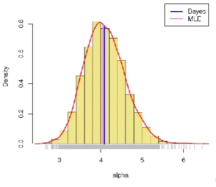
Histograms can provide insights on skewness, behaviour in the tails, presence of multi-modal behaviour, and data outliers; histograms can be compared to the fundamental shapes associated with standard analytic distributions.
[image:5.595.331.541.101.180.2]Histogram and kernel density estimate of and based on MCMC samples, vertical lines represent the corresponding MLE and Bayes estimate.
Figure 8 and 9 provide the kernel density estimate of and . The kernel density estimates have been drawn using R[19,20] with the assumption of Gaussian kernel and properly chosen values of the bandwidths.
[image:5.595.328.530.267.361.2]Fig 6. Sequential realization of the parameters and
Fig 7. The autocorrelation plots for and
[image:5.595.322.536.508.693.2]From the above Figure 8 and 9, It can be seen that and both are symmetric.
5.1.3
Numerical Summary
In Table 2, we have considered various quantities of interest and their numerical values based on MCMC sample of posterior characteristics for Exponentiated Gumbel model under uniform priors. The numerical summary is based on final posterior sample (MCMC output) of 7000 samples for alpha and sigma.
{1i , σ1i}, i = 1,…,7000 from chain 1,
and,
{2i 2i}, i = 1,…,7000 from chain 2.
5.2
Bayesian Analysis under Gamma Priors
The developed module is implemented to obtain the Bayes estimates of the Exponentiated Gumbel model using MCMC method to generate MCMC sample from posterior distribution for given set of gamma priors, which is most widely used prior distribution of is the inverted gamma distribution with parameters a and b (>0) with p.d.f. given by
(a 1) a /
b
e ; 0 (a, b) 0 ( ) (a)
0 ; otherwise
We also run the two parallel chains for sufficiently large number of iterations, say 5000 the burn-in, until convergence results. Final posterior sample of size 7000 is taken by choosing thinning interval five i.e. every fifth outcome is stored and same procedure is adopted for analysis as used in the case of uniform priors.
5.2.1
Convergence diagnostics
Simulation-based Bayesian inference requires using simulated draws to summarize the posterior distribution or calculate any relevant quantities of interest. We need to treat the simulation draws with care.The first step in making an inference from an MCMC analysis is to ensure that an equilibrium distribution has indeed been reached by the Markov chain, i.e., that the chain has converged. For each parameter, we started the chain at an arbitrary point (the initial value or init chosen for each parameter), and because successive draws are dependent on the previous values of each parameter, the actual values chosen for the inits will be noticeable for a while. Therefore, only after a while is the chain independent of the values with which it was started. These first draws ought to be discarded as a burn-in as they are unrepresentative of the equilibrium distribution of the Markov chain.
5.2.1.1 Running Mean (Ergodic mean) Plot
The convergence pattern can be studied by calculating the running mean which is the mean of all sampled values up to and including that at a given iteration. We thus generate a time series(Iteration number) graph of the running mean for each parameter in the chain. The Ergodic mean plots for the parameters shown in figure 10 depict the convergence pattern.
5.2.1.2 Brooks-Gelman-Rubin Diagnostic
Evidence for convergence comes from the red line being close to 1 on the y-axis and from the blue and green lines being stable (horizontal) across the width of the plot.
From the Figure 11, it is clear that convergence is achieved.
[image:6.595.63.279.82.303.2]Fig 9. Histogram and kernel density estimate of
[image:6.595.57.282.443.674.2]Fig 10. The Ergodic mean plots for alpha and sigma.
5.2.2 Visual summary by using Box plots
The boxes represent inter-quartile ranges and the solid black line at the (approximate) centre of each box is the mean; the arms of each box extend to cover the central 95 per cent of the distribution - their ends correspond, therefore, to the 2.5% and 97.5% quantiles. (Note that this representation differs somewhat from the traditional.)
5.2.3 Numerical Summary
In Table 3, we have considered various quantities of interest and their numerical values based on MCMC sample of posterior characteristics for EG model under Gamma priors. The Highest probability density (HPD) intervals are computed the algorithm described by Chen and Shao (1999) under the assumption of unimodal marginal posterior distribution
6. COMPARISON WITH MLE UNDER
UNIFORM PRIORS
For the comparison with MLE, we have plotted two graphs. In Figure 13, the density functions f(x; , ) ˆ ˆ using MLEs and Bayesian estimates, computed via MCMC samples under uniform priors, are plotted.
whereas, Fig.14 represents the Quantile-Quantile(Q-Q) plot of empirical quantiles and theoretical quantiles computed from MLE and Bayes estimates.
Thus, It is clear from the above figures, the MLEs and the Bayes estimates with respect to the uniform priors are quite close and fit the data very well.
7. COMPARISON WITH MLE UNDER
GAMMA PRIORS
[image:7.595.330.532.70.443.2]For the comparison with MLE, we have plotted a graph which exhibits the estimated reliability function which is shown by dashed line using Bayes estimate under gamma priors and the empirical reliability function which is shown by solid line. It is clear from Fig.15, the MLEs and the Bayes estimates with respect to the gamma priors are quite close and fit the data very well.
Fig 12. The boxplots for alpha and sigma.
Fig 13. The density functions f(x; , ) ˆ ˆ using MLEs and Bayesian estimates.
[image:7.595.60.279.163.267.2] [image:7.595.55.280.365.540.2]8. CONCLUSION
The ExponentiatedGumbel model with shape parameter and scale parameter has been discussed and estimate of its parameters obtained based on a complete sample by using the Markov chain Monte Carlo (MCMC) method. The MCMC method has proven more effective as compared to the usual methods of estimation.
Bayesian analysis under different set of priors has been carried in to OpenBUGS to study the convergence pattern. A numerical summary based on MCMC samples of posterior characteristic for Exponented Gumbel model has been worked out under non-informative and informative set of priors. A visual summary under different set of priors which include box plot, kernel density estimation and comparison with MLE has been also attempted and it has been found that the proposed methodology is suitable for empirical modeling and best suited for data set which is considered for illustration under uniform and gamma sets of priors.
9. ACKNOWLEDGMENTS
The authors are thankful to the editor and the referees for their valuable suggestions, which improved the paper to a great extent.
10. REFERENCES
[1]. Gumbel, E.J.(1954). Statistical theory of extreme values and some practical applications. Applied Mathematics Series, 33. U.S. Department of Commerce, National Bureau of Standards.
[2]. Kumar, R., Srivastava, A.K. and Kumar, V. (2012). Analysis of Gumbel Model for Software Reliability Using Bayesian Paradigm, International Journal of Advanced Research in Artificial Intelligence, Vol. 1 (9), 39-45.
[3]. Nadarajah S. (2006). The ExponentiatedGumbel distribution with climate application, Environmetrics 17:13-23
[4]. Persson, K. and Ryd´en, J. (2010). Exponentiated Gumbel Distribution for Estimation of Return Levels of Significant Wave Height, Journal of
[5]. Kumar, V. and Ligges, U. (2011). reliaR : A package for some probability distributions.
http://cran.r-project.org/web/packages/reliaR/index.html.
[6]. Robert, C. P. and Casella, G. (2004). Monte Carlo Statistical Methods, 2nd ed., New York, Springer-Verlag.
[7]. Chen, M., Shao, Q. and Ibrahim, J.G. (2000). Monte Carlo Methods in Bayesian Computation, Springer, NewYork.
[8]. Lawless, J. F., (2003). Statistical Models and Methods for Lifetime Data, 2nd ed., John Wiley and Sons, New York.
[9]. Lyu, M.R., (1996). Handbook of Software Reliability Engineering, IEEE Computer Society Press, McGraw Hill, 1996.
[10].Srivastava, A.K. and Kumar V. (2011). Analysis of Software Reliability Data using Exponential Power Model. International Journal of Advanced Computer Science and Applications, Vol. 2, No. 2, February 2011, 38-45.
[11].Srivastava, A.K. and Kumar V. (2011). Markov Chain Monte Carlo methods for Bayesian inference of the Chen model, International Journal of Computer Information Systems, Vol. 2 (2), 07-14.
[12].Srivastava, A.K. and Kumar V. (2011). Software reliability data analysis with Marshall-Olkin Extended Weibull model using MCMC method for non-informative set of priors, International Journal of Computer Applications, Vol. 18(4), 31-39.
[13].Robert, C. P. and Casella, G. (2004). Monte Carlo Statistical Methods, 2nd ed.,New York, Springer-Verlag.
[14].Chen, M., Shao, Q. and Ibrahim, J.G. (2000). Monte Carlo Methods in BayesianComputation, Springer, NewYork.
[15].Thomas, A. (2010). OpenBUGS Developer Manual, Version 3.1.2, http://www.openbugs.info/.
[16].Thomas, A., O’Hara, B., Ligges, U. and Sturtz, S. (2006). Making BUGS Open, R News, 6, 12-17, http://mathstat.helsinki.fi/openbugs/.
[17].Lunn, D.J., Andrew, A., Best, N. and Spiegelhalter, D. (2000). WinBUGS – A Bayesian modeling framework: Concepts, structure, and extensibility, Statistics and Computing, 10, 325-337.
[18].Kumar, V., Ligges, U. and Thomas, A. (2010). ReliaBUGS User Manual : A subsystem in OpenBUGS for some statistical models, Version 1.0,
OpenBUGS 3.2.1,
http://openbugs.info/w/Downloads/.
[19].Ihaka, R. and Gentleman, R.R. (1996). R: A language for data analysis and graphics, Journal of Computational and Graphical Statistics, 5, 299–314.
[image:8.595.53.265.83.250.2][20].Venables, W. N., Smith, D. M. and R Development Core Team (2010). An Introduction to R, R Foundation for Statistical Computing, Vienna, Austria. ISBN 3-900051-12-7, http://www.r-project.org.
10. AUTHOR’S PROFILE
RAJ KUMAR received his MCA from M.M.M. Engineering College, Gorakhpur and pursuing Ph.D. in Computer Science from D.D.U. Gorakhpur University. Currently working in National Institute of Electronics and Information Technology (formly known as DOEACC Society), Gorakhpur, Ministry of Communication and Information Technology, Government of India.
ASHWINI KUMAR SRIVASTAVA received his M.Sc in Mathematics from D.D.U.Gorakhpur University, MCA(Hons.) from U.P.Technical University, M. Phil in Computer Science from Allagappa University and Ph.D. in Computer Science from D.D.U.Gorakhpur University, Gorakhpur. Currently working as Assistant Professor in Department of Computer Application in Shivharsh Kisan P.G.
College, Basti, U.P. He has got 8 years of teaching experience as well as 4 years research experience. His main research interests are Software Reliability, Artificial Neural Networks, Bayesian methodology and Data Warehousing.