Sample sizes for the SF-6D preference
based measure of health from the SF-36:
a practical guide
Walters, SJ and Brazier, JE
The University of Sheffield
November 2002
HEDS Discussion Paper 02/03
Disclaimer:
This is a Discussion Paper produced and published by the Health Economics and Decision Science (HEDS) Section at the School of Health and Related Research (ScHARR), University of Sheffield. HEDS Discussion Papers are intended to provide information and encourage discussion on a topic in advance of formal publication. They represent only the views of the authors, and do not necessarily reflect the views or approval of the sponsors.
White Rose Repository URL for this paper:
http://eprints.whiterose.ac.uk/10947/
Once a version of Discussion Paper content is published in a peer-reviewed journal, this typically supersedes the Discussion Paper and readers are invited to cite the published version in preference to the original version.
Published paper
None.
The University of Sheffield
ScHARR
School of Health and Related Research
Sheffield Health Economics Group
Discussion Paper Series
November 2002
Ref: 02/3
Sample sizes for the SF-6D preference based measure of health
from the SF-36: a practical guide
Stephen J. Walters*
Lecturer in Medical Statistics
Sheffield Health Economics Group, University of Sheffield
John E. Brazier
Professor of Health Economics
Sheffield Health Economics Group, University of Sheffield
* Corresponding Author:
Sheffield Health Economics Group, School of Health and Related Research University of Sheffield, Regent Court, 30 Regent Street, Sheffield, UK, S1 4DA Tel +44 114 222 0715 Fax +44 114 272 4095
email: [email protected]
ABSTRACT
Background
Health Related Quality of Life (HRQoL) measures are becoming more frequently used in clinical trials and health services research, both as primary and secondary endpoints. Investigators are now asking statisticians for advice on how to plan and analyse studies using HRQoL measures, which includes questions on sample size. Sample size requirements are critically dependent on the aims of the study, the outcome measure and its summary measure, the effect size and the method of calculating the test statistic. The SF-6D is a new single summary preference-based measure of health derived from the SF-36 suitable for use clinical trials and in the economic evaluation of health technologies.
Objectives
To describe and compare two methods of calculating sample sizes when using the SF-6D in comparative clinical trials and to give pragmatic guidance to researchers on what method to use.
Methods
We used bootstrap computer simulation to compare the power of the two methods for detecting a shift in location.
Results
This paper describes the SF-6D and retrospectively calculated parametric and non-parametric effect sizes for the SF-6D from a variety of studies that had previously used the SF-36. Computer simulation suggested that if the distribution of the SF-6D is reasonably symmetric then the t-test appears to be more powerful than the MW test at detecting differences in means. Therefore if the distribution of the SF-6D is symmetric or expected to be reasonably symmetric then parametric methods should be used for sample size calculations and analysis. If the distribution of the SF-6D is skewed then the MW test appears to be more powerful at detecting a location shift (difference in means) than the t-test. However the differences in power (between the t and MW tests) are small and decrease as the sample size increases.
Conclusions
We have provided a clear description of the distribution of the SF-6D and believe that the mean is an appropriate summary measure for the SF-6D when it is to be used in clinical trials and the economic evaluation of new health technologies. Therefore pragmatically we would recommend that parametric methods be used for sample size calculation and analysis when using the SF-6D.
1. INTRODUCTION
Health Related Quality of Life (HRQoL) measures are becoming more frequently used in clinical trials and health services research, both as primary and secondary endpoints. Investigators are now asking statisticians for advice on how to plan and analyse studies using HRQoL measures, which includes questions on sample size. Sample size calculations are now mandatory for many research protocols and are required to justify the size of clinical trials in papers before they will be accepted by journals.1
Thus, when an investigator is designing a study to compare the outcomes of an intervention, an essential step is the calculation of sample sizes that will allow a reasonable chance (power) of detecting a predetermined difference (effect size) in the outcome variable, at a given level of statistical significance. Sample size is critically dependent on the purpose of the study, the outcome measure and how it is summarised, the proposed effect size and the method of calculating the test statistic.
The increasing use of economic evaluation in the assessment of health care interventions has resulted in a growing demand for methods of measuring and valuing health that can be readily used in clinical trials. However, many conventional health-related quality of life measures are not suitable for use in economic evaluation.3 These measures of health status or health related quality of life (HRQoL) are standardised questionnaires used to assess patient health across broad areas such as symptoms, physical functioning, work and social activities, and mental well-being. Responses to items are combined into either a single index or a profile of several sub-indices of scores. Most of these measures of HRQoL are scored using a summation of coded responses to the items. Such instruments have become widely used by clinical researchers and can provide useful descriptive information on the effectiveness of health care interventions. The main shortcoming of using such instruments in economic evaluation is that they do not explicitly incorporate preferences into their scoring algorithms. Another type of instrument is the utility or preference-based measure of health, that combine a descriptive system with preference weights obtained from members of the general population, such as the EQ-5D4 and the Health Utility Index (HUI)5.
The remainder of this paper is structured into the following sections. Section 2 briefly describes the SF-36 measure and the single preference weighted SF-6D index. Section 3 talks about cost-effectiveness analysis. Section 4 summarises the methods and the sample size formulae. Section 5 describes some of the effect sizes that have been observed in previous studies using the SF-6D. The next section (6) compares the different methods of sample size calculation using computer simulation. The final sections (7 and 8) talk about the choice of sample size method with the SF-6D and conclusions.
2. SF-36 HEALTH SURVEY AND THE SF-6D HEALTH STATE CLASSIFICATION
Furthermore the method of scoring the SF-36 is not based on preferences. The simple scoring algorithm for the eight dimensions assumes equal intervals between the response choices, and that all items are of equal importance, which may not be appropriate. Brazier et al10, 11 have derived a preference-based or utility measure of health from the SF-36, called the SF-6D, which reduces all the outcomes to a single summary measure for use in clinical trials and economic evaluations. All responders to the original SF-36 questionnaire can be assigned SF-6D score provided the 11 items used in the six dimensions of the SF-6D have been completed. The SF-6D preference-based measure can be regarded as a continuous outcome scored on a 0.29 to 1.00 scale, with 1.00 indicating "full health".
3. QUALITY ADJUSTED LIFE YEARS AND COST-EFFECTIVENESS ANALYSIS
Preference-based health state scores or utilities do not have natural units. Since health is a function of both length of life and quality of life the QALY (Quality-adjusted life year) has been developed in an attempt to combine the value of these attributes into a single index number. If utilities are multiplied by the amount of time spent in that particular health state then they become QALYs (and are measured in units of time). QALYs allow for varying times spent in different states by calculating an overall score for each patient. If a patient progress through four health states (i= 1 to 4) that have estimated utilities, U1, U2, U3 and U4, spending time Ti in each state then:
QALY = U1T1 + U2T2 + U3T3 + U4T4.
The Central Limit Theorem (CLT)13 suggests that if we have a series of independent, identically distributed random variables, then their sum tends to a Normal distribution as the number of variables increases. Although utilities measured on the same individual are not independent and likely to be serially correlated, the distribution of the ‘sum’ of these utilities (i.e. the AUCs or QALYs), are more likely to be symmetric and a fairly good fit to the Normal. This result implies that parametric methods for both sample calculations and analysis can be used when the outcome is a QALY. Multiple linear regression methods can be used to adjust QALYs for other covariates.14
Cost-effectiveness and Cost Utility Analysis
If information on the resources consumed and the cost of the resources is collected then an economic evaluation may be performed alongside the clinical trial. Cost-effectiveness analysis (CEA) is one form of full economic evaluation, where both the costs and consequences of heath programmes or treatments are examined.15 If we know the expected costs of the standard control treatment (µCC) and the new
experimental treatment (µCT), and similarly their expected effectiveness µEC and µET,
respectively, then differences in costs and effects can be defined as ∆C = µCT – µCC
and ∆E = µET – µEC.
When ∆C > 0 and ∆E > 0 or ∆C < 0 and ∆E < 0, neither the experimental nor standard is dominant, the convention is to examine the incremental cost effectiveness ratio (ICER), R, defined as
E C R
EC ET
CC CT
∆ ∆ = − − =
µ µ
µ µ
The ICER, R measures the extra cost for achieving an extra unit of effectiveness by adopting the experimental treatment over the standard.
In cost-utility analysis (CUA) the incremental cost of a programme, from a particular viewpoint, is compared to the incremental health improvement attributable to the programme, where the health improvement is measured in QALYs gained. The results are usually expressed as a cost per QALY gained.
In the case of preference-based measures one might argue that the ultimate objective is to influence resource allocation decisions.16 Therefore, it is the difference in cost-effectiveness (e.g. incremental cost per QALY) that is important not the change in HRQoL. Hence changes in the HRQoL measure alone may not be of interest without also considering the cost of bringing about those changes. Thus, the sample size calculation if one was performed, would be designed such that it would be possible to assess whether the incremental cost per QALY for the new treatment, compared with the existing one, is within an acceptable interval (e.g. less than £30,000 per QALY). There are several statistical methods for constructing confidence intervals for incremental cost-effectiveness ratios (e.g. Taylor series approximation, Fieller’s Method and the bootstrap).17
If decision makers at the design stage of a study, can specify their maximum threshold willingness to pay for an additional unit of effectiveness, say RMax, and we
have the necessary estimates of ∆C and ∆E, their variances (σ2EC, σ2ET, σ2CC, σ2CT)
and covariances (or the correlation between cost and effects, ρCE). Then using
size n, such that the upper limit of the 95% CI for the R is less than RMax. A strong
limitation of this method is the quantities that must be pre-specified. Even if we assume that the variances of costs and effectiveness respectively are the same in the Treatment and Control groups, we still require more than double the information to calculate a sample size to demonstrate cost-effectiveness, rather than effectiveness alone.
A likely consequence of designing studies to test hypotheses jointly about costs and effects is that the sample required may be larger than that to show differences in effects only. O’Brien19 et al raise an important ethical question: would it be ethical to continue a clinical trial to reach sufficient power to test a cost-effectiveness question when the number to show efficacy has been reached? They suggest a pragmatic way forward in that both the clinical and economic questions can be assessed by the same sample size (n for efficacy), but the investigator must simply accept greater uncertainty and wider 95% confidence intervals for the economic outcomes. Therefore, for the rest of this paper we will consider the estimation of sample sizes for differences in efficacy, not cost-effectiveness.
4. WHICH SAMPLE SIZE FORMULAE?
In principle, there are no major differences in planning a study using the SF-6D as an outcome to those using conventional clinical outcomes. Pocock outlines five key questions regarding sample size:20
1. What is the main purpose of the trial?
2. What is the principal measure of patient outcome?
3. How will the data be analysed to detect a treatment difference? 4. What type of results does one anticipate with standard treatment?
5. How small a treatment difference is it important to detect and with what degree of certainty?
Thus, after deciding on the purpose of the study and the principle outcome measure, the investigator must decide how the data is to be analysed to detect a treatment difference. We must also identify the smallest treatment difference that is of such clinical value that it would be very undesirable to fail to detect it. Given answers to all of the five questions above, we can then calculate a sample size.
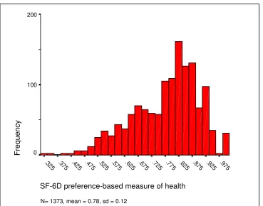
Figure 1 shows the overall distribution of the SF-6D in a general population sample aged 16 to 74 years.7 The SF-6D does not appear to be Normally distributed and appears to be negatively skewed, with more people reporting better health in this general population sample. Conversely Figure 2 shows the distribution of the SF-6D in a group of patients with venous leg-ulcers.22 The distribution of the SF-6D in this group is more symmetric with patients reporting poorer health than the general population sample.
Method 1: Normally distributed continuous data –comparing two means
Suppose we are planning a two-group study comparing HRQoL (using the SF-6D as the primary outcome) between the groups. We believe that the mean difference in SF-6D scores between the two groups is an appropriate comparative summary measure. Therefore using Method 1 and assuming a standard deviation σ of 0.12 and that a mean difference (µET - µEC) of 0.05 or more points between the two groups
is clinically and practically relevant gives a standardised effect size (from equation 2) of 0.417. Using this standardised effect size in equation 3 with a two-sided 5% significance level and 80% power gives the estimated number of subjects per group as 93.
Transformations
are scored on 0.0 to 1.0 scales and the natural logarithm of zero does not exist. Unfortunately log-transforming the general population data in Figure 2 did not make the distribution of the data more symmetric. The mean log-transformed SF-6D score was now -0.27 (SD 0.17).
Equation 3 can now be applied to the log-transformed scale once the standardised effect size δNormal is specified. Unfortunately, there is no simple interpretation for the
log-transformed SF-6D scale, and so the inverse transformation is used to obtain scores corresponding to the original (0.3 to 1.0) SF-6D scale. The mean SF-6D score (on the 0.3 to 1.0 scale) using the inverse transformation is now exp (-0.27) = 0.76 compared to the original value of 0.78.
As before, if, 0.05 unit change on the original SF-6D scale is considered the minimum clinically important difference to detect. Using the log-transformed scale of the SF-6D, a 0.05 increase is approximately from 0.76 to 0.81. This is then expressed as an anticipated effect on the log transformed scale as δNormal = (µET –
µEC)/σΕ = [loge(0.76 + 0.05) – loge(0.76)]/0.17 = 0.37. Using equation 3 with δNormal =
0.37 gives nNormal = 117 patients per group. This can be compared with an
untransformed standardised effect size of 0.42, and an estimated sample size of 93 patients per group.
fact, only the logarithmic transformation gives results interpretable on the original scale.23 The logarithmic transformation expresses the effect as a ratio of the geometric mean for patients in the treatment group to the geometric mean for patients in the control group. This is because the difference between two logarithms is the logarithm of the ratio: log (T) – log (C) = log (T/C).
However, this ratio will vary in a way that depends on the geometric mean value of the control treatment C. For example, if the geometric mean for the control treatment C is 0.6 and treatment T induces a change in SF-6D of 0.10 compared to this level, then this implies an effect size of loge (0.70/0.60) = 0.15. On the other hand, for
geometric mean of 0.8 for the treatment C but the same numerical change of 0.10 implies an effect size of loge (0.9/0.8) = 0.12. Thus, although in this example the
effect size is a 0.10 unit difference in HRQoL in both cases when expressed on the untransformed SF-6D scale, the logarithmic transformation results in a second effect size that is almost 80% (0.12/0.15 = 0.80) of the first. This makes interpretation difficult.
Method 2: Non-normally distributed continuous data
If the SF-6D outcome is assumed to be continuous and plausibly not sampled from a Normal distribution then the most popular (not necessarily the most efficient) non-parametric test for comparing two independent samples is the two-sample Mann-Whitney U (also known as the Wilcoxon rank sum test).24
Suppose we have two independent random samples X1, X2,…,Xm and Y1, Y2,….,Yn
population against the alternative that the Y observations tend to be larger than the X observations. As a test statistic we can use the Mann-Whitney (MW) statistic U, i.e., U = #(Yj > Xi), i = 1,..,m; j = 1,…,n,
which is a count of the number of times the Yjs are greater than the Xis. The
magnitude of U has a meaning, because U/nm is an estimate of the probability that an observation drawn at random from population Y would exceed an observation drawn at random from population X.
Noether25 derived a sample size formula for the Mann-Whitney test (see equation 5 in Table 1), using an effect size pNoether, that makes no assumptions about the
distribution of the data (except that it is continuous), and can be used whenever the sampling distribution of the test statistic U can be closely approximated by the Normal distribution, an approximation that is usually quite good except for very small n.26
Thus to determine the sample size, we have to find the ‘effect size’ pNoether. There are
several ways of estimating pNoether,27 under various assumptions, one possibility is pNoether = U/nm.28 If we let µX, σ2X, µY, and σ2Y be the mean and variance of the X and
Y variables respectively. Then if X ~ N(µX, σ2X) and Y ~ N(µY, σ2Y) then Simonoff et
al27 show that the maximum likelihood estimator of Prob (Y > X) using the sample estimates of the mean and variance ( ˆ , ˆ2, ˆ , ˆ2
Y Y X
X σ µ σ
µ ) is:
(
)
(
)
+
−
Φ
=
>
=
1/22 2
ˆ
ˆ
ˆ
ˆ
ob
Pr
Y X X YX
Y
p
σ
σ
µ
µ
(6),If we assume the SF-6D is Normally distributed then equation 6 allows the calculation of two comparable 'effect sizes' pNoether and δNormal thus enabling the two methods of
sample size estimation (Equations 3 and 5) to be directly contrasted. If this SF-6D is not Normally distributed then we cannot use equation 6 to calculate comparable effect sizes and must rely on the empirical estimates calculated post hoc from the data.
Suppose we are planning a two-group study comparing HRQoL (using the SF-6D as the primary outcome) between the groups. We believe the SF-6D to be continuous, but not Normally distributed and are intending to compare SF-6D scores in the two groups with a Mann-Whitney U test. Therefore Noether's method will be appropriate. As before if we assume a mean difference of 0.05 and a standard deviation of 0.12 for the SF-6D, then using equation 6 this leads to an effect size pNoether = Prob(Y > X)
of 0.616. Substituting pNoether = 0.616 in equation 5 with a two-sided 5% significance
level and 80% power gives the estimated number of subjects per group as 98.
The two methods have given similar sample size estimates. The two methods can be regarded as equivalent when the two distributions have the same shape and equal variances. When the two distributions are Normally distributed with equal variances, the MW test will require about 5% more observations than the two-sample t-test to provide the same power against the same alternative. For non-Normal populations, especially those with long tails, the MW test may not require as many observations as the two-sample t-test. 29
Some allowance should be made for a proportion of subjects who withdraw or are lost to a study during the course of the investigation. If a proportion, θ, are lost so that the outcome (SF-6D) is not recorded, then the final analysis will be based on 1 - θ times the number of subjects entering the study. To ensure an adequate sample size at the end of the study it would be necessary to start with a sample size n’, given by14
θ − = ′
1
n
n (7),
where n is the sample size determined by the methods given earlier in this section.
5. EFFECT SIZES
There is general agreement that further research is required to establish what are realistic and clinically meaningful effect sizes for the SF-36 and SF-6D. To date two broad strategies have been used to interpret differences or changes in HRQoL following treatment:30
1. Distribution based approaches - the effect size (ES);
2. Anchor-based measures - the minimum clinically important difference (MCID).
Anchor-based methods examine the relationship between an HRQoL measure and an independent measure (or anchor) to elucidate the meaning of a particular degree of change. One anchor-based approach uses an estimate of the MCID, the difference on the HRQoL scale corresponding to self-reported small but important change on a global scale.32
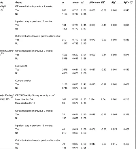
We used a distribution-based approach to determine the observed effect sizes (both Cohen's and Noether's), using the SF-6D, for a variety of studies including randomised controlled trials,33 34 cross-sectional surveys7 35 and observational studies.36, 37, 38, 39 Tables 2, 3 and 4 show the observed effect sizes (both Cohen's and Noether's), and that most of the standardised effect sizes (δNormal) using Cohen's
criteria are in the small to moderate interval. The information on mean differences, standard deviations and effect sizes shown in the tables may be helpful when estimating sample sizes for future studies using the SF-6D. To illustrate the various methods of sample size calculation we assumed a mean difference of 0.05 in SF-6D scores was the MCID difference worth detecting, although further empirical research is require to determine this. Research on the HUI has suggested that a difference of 0.03 is considered important.16 A number of studies in a variety of disease areas have suggested that the MCID appears to average approximately 0.5 on a seven-point scale or 1 part in 14. 32, 40, 41With the SF-6D’s minimum and maximum of 0.29 to 1.00 (i.e. a range of 0.71), one-fourteenth of the scale equates to 0.05.
6. COMPARISON OF THE TWO METHODS OF SAMPLE SIZE ESTIMATION
a computer intensive method for statistical analysis.43 It involves repeatedly drawing random samples from the original data, with replacement. It seeks to mimic in an appropriate manner the way the sample is collected from the population in the bootstrap samples from the observed data. The ‘with replacement’ means that any observation can be sampled more than once.
Suppose (as before) we have two independent random samples X1, X2,…,Xm and Y1,
Y2,….,Yn. The Xs are Ys are random samples from continuous distributions having
cumulative distribution functions, FX and FY respectively. We will consider situations
where the distributions have the same shape, but the locations may differ. Thus if d denotes the location difference (i.e. mean (Y) - mean (X) = d), then FY(y) = FX(y - d),
for every y. We shall focus on the null hypothesis H0: d = 0 against the alternative HA:
d > 0. We can test these hypotheses using an appropriate significance test (e.g. Mann-Whitney or t-test), and will let π (F, d, α, n ) denote the power function of the test.
The bootstrap strategy is to use pilot data to a provide a non-parametric estimate of F and to use a simulation method for finding the power of the test associated with any specified sample size n if the data follow the estimated distribution function. If we denote the distribution function estimate by G, under the alternative hypothesis d, we can estimate the approximate power, πˆ
(
G,d,α,n)
by the following computer simulation procedure.26,42X1*,…,Xn*. Then d is added to each of the other n observations in the sample
to form the simulated sample of Y's, denoted by Y1*,…,Yn*. (The Y*'s and X*'s
have been generated from the same distribution except that the distribution of the Y*'s is shifted d units to the right.)
2. The test statistic (Mann-Whitney or t-test) is calculated for the X*'s and Y*'s, yielding T*. If T* ≥ T1-α/2, (where T1-α/2 is the critical value of the test statistic) a
success is recorded; otherwise a failure is recorded.
3. Steps 1 and 2 are repeated J times. The estimated power of the test,
(
G,d, ,n)
ˆ α
π , is approximated by the proportion of successes among the J
repetitions. (In all cases discussed in this paper, J = 10,000).
The software Resampling Stats was used for the bootstrapping.44 The bootstrap computer simulation procedure involved separately using two datasets. The first used SF-6D data from a general population survey based on 1373 people aged 16-74 years as the pilot dataset.7 Figure 1 shows the non-symmetric distribution of the SF-6D. The second pilot data used SF-6D data from a sample of 232 patients with venous leg-ulcers. 22 Figure 2 shows the more symmetric distribution of the SF-6D in the leg ulcer sample.
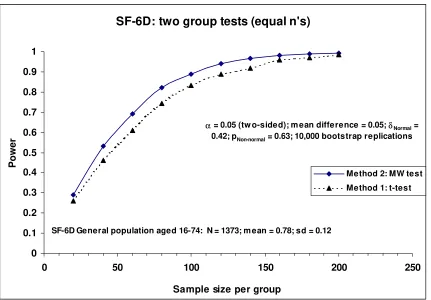
Figure 3 shows the estimated power curves for the t and Mann-Whitney tests at the 5% two-sided significance level for detecting a location shift (mean difference) d = 0.05 in the SF-6D general population data for sample sizes per group varying from 20 to 240. For these general population data a location shift of d = 0.05 is equivalent to a standardised effect size δNormal = 0.42 and pNoether = Prob (Y > X) = 0.63. For a
compared to an estimated power of 0.83 for the t-test. The Mann-Whitney test appears to be more powerful at detecting a location shift of d = 0.05 than the t-test. So for the general population data (with its skewed SF-6D distribution) the MW test is preferable to the t-test. Therefore for a fixed power, significance level and effect size using Noether’s method would produce the smaller sample size estimates. However the differences in power are small and decrease as the sample size increases.
Figure 4 shows that for the leg-ulcer data (with their more symmetric SF-6D distribution), the t-test appears to be slightly more powerful at detecting a location shift of d = 0.05 than the MW test. For these data a location shift of d = 0.05 is equivalent to a standardised effect size δNormal = 0.38 and pNoether = Prob (Y > X) =
0.61. However again the differences in power between the t-test and MW tests are small and decrease as the sample size increases.
7. CHOICE OF SAMPLE SIZE METHOD WITH THE SF-6D OUTCOMES
It is important to make maximum use of the information available from other related studies or extrapolation from other unrelated studies. The more precise the information the better we can design the trial. We would recommend that researchers planning a study with SF-6D as the primary outcome pay careful attention to any evidence on the validity and frequency distribution of the SF-6D.
slightly more powerful than the Mann-Whitney test at detecting differences in means. Therefore if the distribution of the SF-6D is symmetric or expected to be reasonably symmetric then parametric methods should be used for sample size calculations and analysis. The use of parametric methods for analysis (i.e. t-test) also enables the relatively easy estimation of confidence intervals, which is regarded as good statistical practice.1
If the distribution of the SF-6D is skewed then the Mann-Whitney test appears to be more powerful at detecting a location shift (difference in means) than the t-test. So in these circumstances the MW test is preferable to the t-test and non-parametric methods could be used for sample size calculations and analysis. However the differences in power (between the t and MW tests) are small and decrease as the sample size increases. The use of non-parametric methods for sample size estimation requires the effect size to be defined in terms of P (Y > X), which is difficult to quantify and interpret. The arithmetic mean and mean difference is a better summary measure for heath care providers in deciding whether to offer a new treatment or not to its population. The mean provides information about the total benefit or utility from treating all patients, which is needed as the basis for health care policy decisions.45 Therefore pragmatically we would recommend that parametric methods be used for sample size calculation and analysis when using the SF-6D in clinical trials and economic evaluations.
the SF-6D outcome, then pragmatically there is no need to worry about the distribution of the SF-6D outcome and we can use equation (3) to calculate sample sizes. Although the Normal distribution is strictly only the limiting form of the sampling distribution of the sample mean as the sample size n increases to infinity, but it provides a remarkably good approximation to the sampling distribution even when n is small and the distribution of the data is far from Normal.14 Generally, if n is greater than 25, these approximations will be good. However, if the underlying distribution is symmetric, unimodal, and of the continuous type, a value of n as small as 4 can yield a very adequate approximation.13
There maybe considerable uncertainties in estimates of such quantities as the standard deviation and the treatment effect. (Although the data displayed in Tables 2 to 4 may be useful). Sample size calculations are sometimes based on estimates “pulled out of thin air”. If an investigator is uncomfortable with the assumptions then it is good practice to calculate sample sizes under a variety of scenarios so that the sensitivity to assumptions can be assessed. We would recommend that various anticipated benefits be considered, ranging from the optimistic to the more realistic, with sample sizes being calculated for several scenarios within that range. It is a matter of judgement, rather than an exact science, as to which of the options is chosen for the final study size.9
In this paper we have concentrated on the issue that HRQoL outcome data (such as the SF-6D) may not meet the distributional requirements of parametric methods of sample size estimation and statistical analysis. There are other equally important problems with HRQoL measures such as ordinal scaling, linearity of the scale, floor/ceiling effects, non-constant variance and missing data which are discussed more fully in Walters et al 2001.4647
8. CONCLUSIONS
clinical trials and the economic evaluation of new health technologies. Therefore pragmatically we would recommend that parametric methods be used for sample size calculation and analysis when using the SF-6D.
Figure 1: Histogram of the SF-6D in the Sheffield population aged 16-747
SF-6D preference-based measure of health
.975 .925 .875 .825 .775 .725 .675 .625 .575 .525 .475 .425 .375 .325
N= 1373, mean = 0.78, sd = 0.12
Frequency
200
100
0
Figure 2: Histogram of the SF-6D in patients with leg-ulcers22
SF-6D preference-based measure of health
1.000 .950 .900 .850 .800 .750 .700 .650 .600 .550 .500 .450 .400 .350 .300
n = 233, mean =0.65, sd = 0.13
Frequency
30
20
10
Figure 3: Estimated power curve for the SF-6D using general population data7
SF-6D: two group tests (equal n's)
0 0.1 0.2 0.3 0.4 0.5 0.6 0.7 0.8 0.9 1
0 50 100 150 200 250
Sample size per group
Power
Method 2: MW test Method 1: t-test
α = 0.05 (tw o-sided); m ean difference = 0.05; δNormal = 0.42; pNon-normal = 0.63; 10,000 bootstrap replications
[image:30.595.77.506.454.755.2]SF-6D General population aged 16-74: N = 1373; m ean = 0.78; sd = 0.12
Figure 4: Estimated power curve for the SF-6D using leg ulcer data22
SF-6D: two group test (equal n's)
0 0.1 0.2 0.3 0.4 0.5 0.6 0.7 0.8 0.9 1
0 50 100 150 200 250
Sample size per group
Power
Method 2: MW test Method 1: t-test
α = 0.05 (tw o-sided); m ean difference= 0.05; δNormal = 0.38; pNon-normal = 0.61; 10,000
bootstrap replications
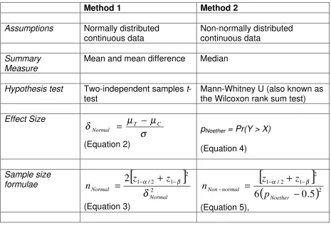
Table 1: Effect size and sample size formulae
Method 1 Method 2
Assumptions Normally distributed continuous data
Non-normally distributed continuous data
Summary Measure
Mean and mean difference Median
Hypothesis test Two-independent samples t-test
Mann-Whitney U (also known as the Wilcoxon rank sum test) Effect Size
σ
µ
µ
δ
T CNormal
−
=
(Equation 2)
pNoether = Pr(Y > X) (Equation 4)
Sample size
formulae
[
]
2 2 1 2 / 1
2
Normal Normalz
z
n
δ
β α − −+
=
(Equation 3)[
]
(
)
22 1 2 / 1
5
.
0
6
−
+
=
− − − Noether normal Nonp
z
z
n
α β(Equation 5),
δNormal is the standardised effect size index, µT and µC are the expected group means of outcome variable under the null and alternative hypotheses and σ is the standard deviation of outcome variable (assumed the same under the null and alternative hypotheses).
pNoether is an estimate of the probability that an observation drawn at random from population Y would exceed an observation drawn at random from population X.
z1-α/2 and z1-βare the appropriate values from the standard Normal distribution for the 100 (1 -
α/2) and 100 (1 - β) percentiles respectively.
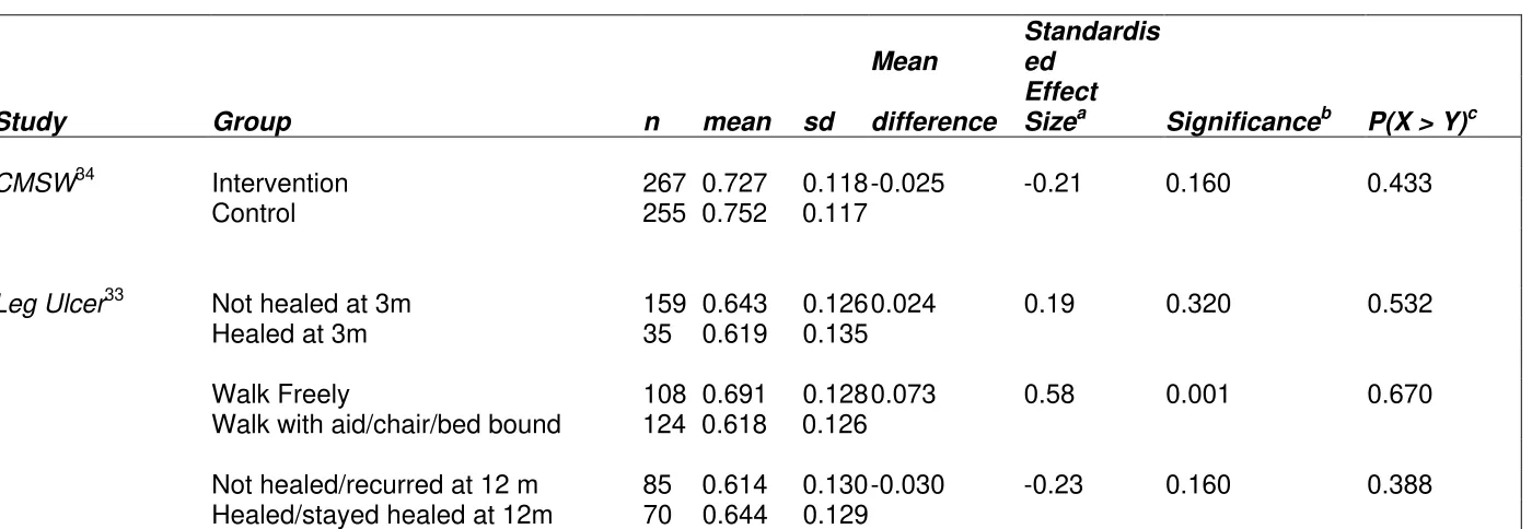
Table 2: Effect sizes – randomised controlled trial
Mean
Standardis
ed
Study Group n mean sd difference
Effect
Sizea Significanceb P(X > Y)c
CMSW34 Intervention 267 0.727 0.118 -0.025 -0.21 0.160 0.433
Control 255 0.752 0.117
Leg Ulcer33 Not healed at 3m 159 0.643 0.126 0.024 0.19 0.320 0.532
Healed at 3m 35 0.619 0.135
Walk Freely 108 0.691 0.128 0.073 0.58 0.001 0.670
Walk with aid/chair/bed bound 124 0.618 0.126
Not healed/recurred at 12 m 85 0.614 0.130 -0.030 -0.23 0.160 0.388
Healed/stayed healed at 12m 70 0.644 0.129
CMSW (Community Midwifery Support Worker) study.
a. Standardised effect size = mean difference divided by the pooled standard deviation. b. Based on a two-independent samples t-test.
Study Group n mean sd difference ESa Sigb P(X > Y)c
Sheffield GP consultation in previous 2 weeks:
16-747 Yes 283 0.716 0.131 -0.070 -0.59 0.001 0.343
No 1183 0.786 0.115
Inpatient stay in previous 12 months:
Yes 164 0.726 0.145 -0.053 -0.44 0.001 0.394
No 1306 0.779 0.117
Outpatient attendance in previous 3 months:
Yes 210 0.712 0.138 -0.072 -0.60 0.001 0.346
No 1247 0.783 0.115
Sheffield Elderly GP consultation in previous 2 weeks:
65+35 Yes 1586 0.622 0.131 -0.060 -0.44 0.001 0.371
No 5329 0.682 0.138
Lives Alone
Yes 2579 0.651 0.140 -0.027 -0.20 0.001 0.442
No 4359 0.678 0.138
Current smoker
Yes 1179 0.656 0.141 -0.015 -0.11 0.001 0.467
No 5748 0.670 0.139
Elderly Sheffield OPCS Disability Survey severity scored
Women 70+ 37 Less disabled 0-4 169 0.701 0.123 0.124 1.04 0.001 0.218
More disabled 5-10 96 0.577 0.113
GP consultation in previous 2 weeks:
Yes 75 0.621 0.110 -0.048 -0.37 0.008 0.398
No 190 0.669 0.139
Inpatient stay in previous 12 months:
Yes 40 0.614 0.138 -0.051 -0.38 0.029 0.409
No 216 0.665 0.133
Outpatient attendance in previous 3 months:
Yes 79 0.627 0.139 -0.043 -0.33 0.015 0.420
No 185 0.671 0.128
GP (General practitioner), OPCS (Office of Population, Censuses and Surveys).
a. ES (Standardised Effect size) = mean difference divided by the pooled standard deviation. b. Sig (Significance) based on a two-independent samples t-test.
c. Based on U/nm, where U = MW test statistic.
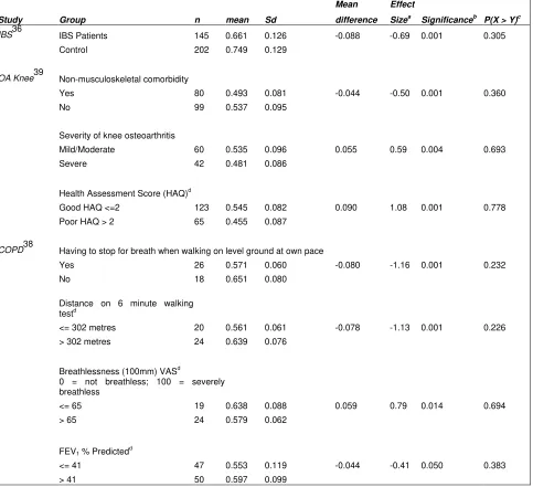
[image:33.595.67.539.74.593.2]Table 4: Effect sizes – longitudinal observation studies
Mean Effect
Study Group n mean Sd difference Sizea
Significanceb
P(X > Y)c
IBS36 IBS Patients 145 0.661 0.126 -0.088 -0.69 0.001 0.305
Control 202 0.749 0.129
OA Knee39 Non-musculoskeletal comorbidity Yes 80 0.493 0.081 -0.044 -0.50 0.001 0.360
No 99 0.537 0.095
Severity of knee osteoarthritis
Mild/Moderate 60 0.535 0.096 0.055 0.59 0.004 0.693
Severe 42 0.481 0.086
Health Assessment Score (HAQ)d
Good HAQ <=2 123 0.545 0.082 0.090 1.08 0.001 0.778
Poor HAQ > 2 65 0.455 0.087
COPD38 Having to stop for breath when walking on level ground at own pace Yes 26 0.571 0.060 -0.080 -1.16 0.001 0.232
No 18 0.651 0.080
Distance on 6 minute walking
testd
<= 302 metres 20 0.561 0.061 -0.078 -1.13 0.001 0.226
> 302 metres 24 0.639 0.076
Breathlessness (100mm) VASd
0 = not breathless; 100 = severely
breathless
<= 65 19 0.638 0.088 0.059 0.79 0.014 0.694
> 65 24 0.579 0.062
FEV1 % Predicted d
<= 41 47 0.553 0.119 -0.044 -0.41 0.050 0.383
> 41 50 0.597 0.099
IBS (Irritable Bowel Syndrome), OA (Osteo-Arthritis), COPD (Chronic Obstructive Pulmonary Disease), a. Standardised effect size = mean difference divided by the pooled standard deviation.
b. Based on a two-independent samples t-test. c. Based on U/nm, where U = MW test statistic.
REFERENCES
1
Altman D.G., Machin D., Bryant T.N., Gardner M.J. Statistics with Confidence. Confidence
intervals and statistical guidelines. 2nd edition. London: British Medical Journal, 2000. 2
Machin D., Campbell M.J., Fayers P.M., Pinol A.J.Y. Sample Sizes Tables for Clinical
Studies. 2nd edition. Oxford: Blackwell Science, 1997. 3
Brazier J., Deverill M., Green C., Harper R., Booth A. A review of the use of health status
measures in economic evaluations. Health Technol Assess 1999; 3 (9); 1-164. 4
Williams A. The measurement and valuation of health: a chronicle. Centre for Health
Economics Discussion paper 136, University of York, 1995. 5
Feeny D., Furlong W., Boyle M., Torrance G.W. Multi-attribute health status classification systems. Health Utilities Index. Pharmacoeconomics 1995; 7: 490-502.
6
Ware J.E. Jr., Sherbourne C.D. The MOS 36-item short-form health survey (SF-36). I. Conceptual framework and item selection. Medical Care 1992; 30: 473-483.
7
Brazier J.E, Harper R., Jones N.M.B., O’Cathain A., Thomas K.J., Usherwood T., Westlake
L. Validating the SF-36 health survey questionnaire: new outcome measure for primary care. British Medical Journal 1992; 305: 160-4.
8
Ware J.E Jr, Kosinski M., Keller S.D. (1994) SF-36 Physical and Mental Health Summary
Scales: A User’s Manual. Health Institute, Boston. 9
Fayers P.M., Machin D.M. Quality of Life: Assessment, Analysis & Interpretation.
Chichester: Wiley, 2000. 10
Brazier J., Usherwood T., Harper R., Thomas K. Deriving a Preference-based Single Index from the UK SF-36 Health Survey. J Clin Epidemiol. 1998; 51(11): 1115-1128.
11
Brazier J.E., Roberts J.F., Deverill M.D. The estimation of a preference based measure of health from the SF-36. Health Economics 2002; 21: 271-292.
12
Matthews J.N.S., Altman D.G., Campbell M.J., Royston P. Analysis of serial measurements in medical research. British Medical Journal 1990; 300; 230-235.
13
Hogg R.V., Tanis E.A. Probability and Statistical Inference. 3rd edition. New York: Macmillan, 1988.
14
Armitage P., Berry G., Matthews J.N.S. Statistical Methods in Medical Research. 4th edition. Oxford: Blackwell Science, 2002.
15
Drummond M.F., Stoddard G.L., Torrance G.W. Methods for the Economic Evaluation of Health Care Programmes. 2nd edition, Oxford: Oxford University Press, 1997.
16
17
Briggs A.H., Mooney C.Z., Wonderling D.E. Constructing Confidence Intervals for Cost-effectiveness ratios: An Evaluation of Parametric and Non-Parametric Techniques Using
Monte Carlo Simulation. Statistics in Medicine 1999; 18: 3245-3262. 18
Willan A.R., O’Brien B.J. Sample size and power issues in estimating incremental
cost-effectiveness ratios from clinical trials data. Health Economics 1999; 8(3): 203-211. 19
O’Brien B.J., Drummond M.F. Labelle R.J., Willan A. In Search of Power and Significance:
Issues in the Design and Analysis of Stochastic Cost-Effectiveness Studies in Health Care. Medical Care 1994; 32(2): 150-163.
20 Pocock S.J. Clinical Trials: A Practical Approach. Chichester: Wiley, 1983. 21
Campbell M.J., Julious S.A., Altman D.G. Estimating sample sizes for binary, ordered categorical, and continuous outcomes in two group comparisons. British Medical Journal
1995; 311: 1145-1148. 22
Walters S.J., Morrell C.J., Dixon S. Measuring health-related quality of life in patients with venous leg ulcers. Quality of Life Research 1999; 8(4): 327-336.
23
Bland J.M., Altman D.G. The use of transformation when comparing two means. British
Medical Journal 1996; 312: 1153. 24
Lehman E.L. Nonparametric Statistical Methods Based on Ranks. San Francisco:
Holden-Day, 1975. 25
Noether G.E. Sample Size Determination for Some Common Nonparametric Tests. J. American Statistical Association 1987; 82(398): 645-647.
26
Collings B.J., Hamilton M.A. Determining the Appropriate Sample Size for Nonparametric Tests for Location Shift. Technometrics 1991; 3(33): 327-337.
27
Simonoff J.S., Hochberg Y., Reiser B. Alternative Estimation Procedures for Pr(X < Y) in Categorised Data. Biometrics 1986; 42: 895-907.
28
Lesaffre E., Scheys I., Frohlich J., Bluhmki E. Calculation of power and sample size with bounded outcome scores. Statistics in Medicine 1993; 12: 1063-1078.
29
Elashoff J.D. nQuery Advisor Version 3.0 User’s Guide. Los Angeles: Statistical Solutions, 1999.
30
Norman G.R., Sridhar F.G., Guyatt G.H., Walter S.D. The Relation of Distribution- and Anchor-Based Approaches in Interpretation of Changes in Health Related Quality of Life.
Medical Care, 2001; 39(10): 1039-1047. 31
Cohen J. Statistical Power Analysis for the Behavioural Sciences. 2nd edition. New Jersey: Lawrence Earlbaum, 1988.
32
33
Morrell C.J., Walters S.J., Dixon S., Collins K.A., Brereton L.M.L., Peters J., Brooker C.G.D. Cost-effectiveness of community leg ulcer clinics: randomised controlled trial. British
Medical Journal 1998; 316: 1487-1491. 34
Morrell C.J., Spiby H., Stewart P., Walters S., Morgan A. Costs and effectiveness of community postnatal support workers: randomised controlled trial. British Medical Journal 2000; 321: 593-8.
35
Walters S.J., Munro J.F., Brazier J.E. Using the SF-36 with older adults: cross-sectional community based survey. Age & Ageing 2001; 30: 337-343.
36
Akehurst R.L., Brazier J.E., Mathers N., Healy C., Kaltenthaler E., Morgan A.M., Platts, M., Walters S.J. Health-related Quality of Life and Cost Impact of Irritable bowel Syndrome in a UK Primary Care Setting. Pharmacoeconomics 2002; 20(7): 455-462.
37
Brazier J.E., Walters S.J., Nicholl J.P., Kohler B. Using the SF-36 and Euroqol on an elderly population. Quality of Life Research 1996; 5: 195-204.
38
Harper R., Brazier J.E., Waterhouse J.C., Walters S.J., Jones N.M.B., Howard P. Comparison of outcome measures for patients with chronic obstructive pulmonary disease
(COPD) in an outpatient setting. Thorax 1997; 52: 879-887. 39
Brazier J.E., Harper R., Munro J.F., Walters S.J., Snaith M.L. Generic and
condition-specific outcome measures for people with osteoarthritis of the knee. Rhemautology 1999; 38: 870-877.
40
Redelmeier D.A. Guyatt G.H., Goldstein R.S. Assessing the minimal important difference in symptoms: a comparison of two techniques. J. Clinical Epidemiology 1996; 49:
1215-1219. 41
Juniper E.F., Guyatt G.H., Feeny D.H. Measuring quality of life in children with asthma. Quality of Life Research 1996; 5: 35-46.
42
Collings B.J., Hamilton M.A. Estimating the Power of the Two-Sample Wilcoxon Test for Location Shift. Biometrics 1998; 44: 847-860.
43
Efron B., Tibshirani R.J. An Introduction to the Bootstrap. New York: Chapman & Hall, 1993.
44
Simon J.L. Resampling Stats: Users Guide. v5.02. Arlington: Resampling Stats Inc, 2000.
45 Thompson S.G., Barber J.A. How should cost data in pragmatic randomised trials be
analysed? British Medical Journal 2000; 320: 1197-1200. 46
Walters S.J., Campbell M.J., Lall R. Design and Analysis of Trials with Quality of Life as an Outcome: a practical guide. Journal of Biopharmaceutical Statistics 2001: 11(3) 155-176. 47
Walters S.J., Campbell M.J., Paisley S. Methods for determining sample sizes for studies involving quality of life measures: a tutorial. Health Services & Outcomes Research
48