Lancaster University Management School
Working Paper
2005/027
A Deterministic Tabu Search Algorithm for the Capacitated
Arc Routing Problem (CARP)
Richard W Eglese and José Brandão
The Department of Management Science Lancaster University Management School
Lancaster LA1 4YX UK
© Richard W Eglese and José Brandão All rights reserved. Short sections of text, not to exceed two paragraphs, may be quoted without explicit permission,
provided that full acknowledgement is given.
The LUMS Working Papers series can be accessed at http://www.lums.lancs.ac.uk/publications/
A Deterministic Tabu Search Algorithm for the Capacitated Arc Routing
Problem (CARP)
José Brandão1* and Richard Eglese2
1. Dep. de Gestão, Escola de Economia e Gestão, Universidade do Minho, Largo do Paço, 4704 -553 Braga, Portugal. email: [email protected]
2. Department of Management Science, Lancaster University Management School, Lancaster, LA1 4YX, United Kingdom. email: [email protected]
* Corresponding Author
Abstract
The Capacitated Arc Routing Problem (CARP) is a difficult optimisation problem in vehicle routing with applications where a service must be provided by a set of vehicles on specified roads. A heuristic algorithm based on Tabu Search is proposed and tested on various sets of benchmark instances. The computational results show that the proposed algorithm produces high quality results within a reasonable
computing time. Some new best solutions are reported for a set of test problems used in the literature.
Keywords
Heuristics, Arc Routing, Tabu Search
1. Introduction
The Capacitated Arc Routing Problem (CARP) may be described as follows: consider
an undirected graph G = (V,E), with a set of required edges R ⊆ E. A vehicle must
service the required edges. A fleet of identical vehicles, each of capacity Q, is based at
a designated depot node. Each edge of the graph (vi, vj) incurs a cost cij whenever a
vehicle travels over it or services it. When a vehicle travels over an edge without
servicing it, this is referred to as deadheading. Each required edge of the graph (vi, vj)
has a demand quantity of qij associated with it. A vehicle route must start and finish at
exceed the capacity of the vehicle, Q. The objective of the CARP is to find a
minimum cost set of vehicle routes where each required edge is serviced on one of the routes.
In the instances tested, the objective is to minimise the total cost incurred on the routes and does not include any costs relating to the number of routes or vehicles required.
The graph or network on which the problem is based may be directed or undirected or mixed, but in this paper only undirected graphs are considered. A good introduction to and survey of the CARP and other arc routing problems may be found in Dror (2000).
In the CARP, each edge in the graph may model a road that can be travelled in either direction and each vertex or node corresponds to a road junction. Applications of the CARP arise in applications such as postal deliveries, household waste collection, winter gritting, snow clearance and others, though in most practical applications there are additional constraints (e.g. time window constraints or restrictions on certain turns) that must also be considered.
The CARP is NP-Hard. Even when a single vehicle is able to service all the required edges, the problem reduces to the Rural Postman Problem which has been shown to be NP-Hard by Lenstra and Rinnooy Kan (1976). Additionally, Golden and Wong (1981) showed that even 1.5-approximation for the CARP is NP-Hard. Exact methods for the CARP have only been able to solve relatively small examples to optimality.
There are also other notable contributions that have recently been proposed for solving the CARP. Beullens et al. (2003) describe a guided local search heuristic for the CARP. Greistorfer (2002) also uses a Tabu Search based approach, but uses a form of scatter search within his proposed heuristic. Hertz and Mittaz (2001) describe a variable neighbourhood descent algorithm for the CARP. Amberg et al. (2000) have also proposed a Tabu Search based algorithm; their approach makes use of
capacitated trees and can be applied to multi-depot problems.
The approach described in this paper is based on a Tabu Search algorithm. However it differs from CARPET in many of the details of the implementation. In particular, the algorithm presented here is deterministic and does not require the use of random parameter values (which are also needed for MA), so making the results fully reproducible.
The structure of the remainder of this paper is as follows. Section 2 describes the methods used to obtain initial feasible solutions in our algorithm. Section 3 describes the Tabu Search algorithm for solving the CARP and Section 4 describes the results obtained on a set of test problems. Final conclusions are presented in Section 5.
2. Initial Solutions
Five different methods were used to obtain initial solutions. Each method provided a feasible solution that could be used as an initial solution for the Tabu Search
algorithm. The methods were designed to be fast to compute and to provide a variety of starting solutions for the Tabu Search algorithm to improve. The diversity provided by the different starting solutions was found to be useful in ultimately finding high quality solutions.
2.1 Method 1 – Cheapest edge
depot to the nearest vertex of that edge along the least cost path (unless the first required edge is adjacent to the depot node). The route is built up by adding edges that are feasible to the end of the route. The next edge to be added is the required edge that has not yet been included in a route which is nearest to the end vertex of the last included edge (and which has least cost in the event of ties), but excluding any edge that closes the tour unless no others are feasible. If the next edge does not share a vertex with the last edge, the route includes the vehicle deadheading edges on the least cost path between the last edge and the next edge. When no remaining required edges can be feasibly added to a route, the route is completed by the vehicle returning to the depot along the least cost path from the end of the last serviced edge, and the next route is started.
2.2 Method 2 – Dearest edge
This method operates in exactly the same way as Method 1, except that the highest cost edge replaces the lowest cost edge at each selection point.
2.3 Method 3 – Insert
Each route is started as in Method 1 and a route is completed by adding the
deadheading path from the end of the first edge back to the depot. Then the next edge to be chosen from the required edges not yet served and which is feasible in terms of vehicle capacity is the one that increases the cost of the route by the least amount. When considering an edge for insertion, the new edge may be inserted between any pair of required edges already included in the route that are currently linked by a deadheading path, or before the first edge or after the last edge if these edges are not directly linked to the depot.
2.4 Method 4 – Connected components
connected, the RPP is polynomially solvable. A general heuristic for the RPP was first proposed in Frederickson (1979), based on a procedure that is similar to Christofides’ heuristic for the undirected travelling salesman problem (Christofides, 1976). The method has been described and used by several researchers; our version follows the version described in Pearn and Wu (1995) (though in that paper it is referred to as “Christofides et al. algorithm”).
Frederickson’s algorithm is described in general here as it is also used within the Tabu Search algorithm to improve individual routes. In what follows, the set of required
edges ER⊆ R refers to the required edges in a connected component for this initial
solution method, or the required edges serviced on one particular route when used within the Tabu Search algorithm. Frederickson’s algorithm may be described as follows:
1. Let GR = (VR, ER) be the subgraph of G containing the required edges ER and the
corresponding set of nodes VR. Let C1, ..., Cc denote the subgraphs of GR that contain
the connected components of ER. Let GC be the graph created by considering each
component as a node. The cost of an edge (i, j)∈GC is defined as d(i, j) = d(Ci, Cj) =
minx, y {d(x, y) - ux - uy}, where x, y ∈V , x∈C1, y∈C2 and ux = - η(deg(x) - 2).
d(x,y) is the cost of the minimum cost path from x to y in the original graph G and
deg(x) is the degree of node x in the original graph G.
2. Determine the minimum cost spanning tree in GC. Let ET be the set of edges from
the minimum cost spanning tree solution.
3. Considering the graph GR ∪ET find a minimum cost perfect matching of the odd
degree vertices. Let EM be the edges of the matching.
4. Find an Eulerian tour in the graph GR ∪ET ∪EM. This tour is the RPP solution.
Pearn and Wu show how the results can be influenced by the use of a parameter η. In
our implementation, the algorithm is executed with η = 0, then η = 1 and the better
solution is chosen.
algorithm was not available and so a simple greedy heuristic was used for the matching step, which can be described as follows:
Step 0. Set every node as non-included.
Step 1. Select the edge with the minimum cost among all the edges of the graph, linking two non-included nodes. Set the two end vertices of this edge as included.
Step 2. Repeat step 1 until all the vertices are included.
If the number of nodes were less than or equal to six, then the heuristic was not applied and the optimum solution was found by complete enumeration. Tests were carried out to see what effect the use of this procedure had on the solution to the CARP by finding the optimum solution to the matching problem by complete enumeration in all cases. As expected, the complete enumeration method was much slower than the procedure using the heuristic, but surprisingly, the average solutions to the CARP were worse than when the heuristic was used. We therefore retained the heuristic procedure for solving the matching problem.
2.5 Method 5 – Path Scanning
This method is based on the procedure proposed by Golden et al (1983). Each route is extended by one required edge at each step using a variety of selection rules.
Each route starts at the depot node. Let S be the set of required edges closest to the
end of the current route that are not yet served and do not exceed the capacity of the
current route. If S is empty then complete the current route using the shortest
deadheading path from the end of the current route to the depot node and start a new
route. If S is not empty, exclude from S any edges that would close the route unless
that would make S empty. Select a required edge in S to be the next edge in the route
to be serviced according to the current rule and extend the current route to the vertex at the end of the selected edge.
Five rules are used to determine the next required edge, e, in the route to be serviced:
1) maximise the distance to the depot, 2) minimise the distance to the depot, 3) use rule 1 if the vehicle is less than half-full, else use rule 2, 4) maximise the ratio
d(e)/c(e), where d(e) and c(e) are, respectively, the demand and the cost of e, 5) minimise this ratio. Each criterion gives rise to one solution and the best of the five is chosen.
Some results to show the effectiveness of these initial solution methods are given in Section 4.
3. The Tabu Search Algorithm
3.1 Neighbourhood Moves
The Tabu Search algorithm (TSA) is based on two types of neighbourhood move. The first is an insertion and the second is a swap.
adjacent, but are linked by a deadheading path of edges. The trial insertion considers both directions for the edge to be traversed when inserted in the new route.
The swap move is similar. Two candidate edges are selected from two different routes, each containing deadheading paths. The candidate edges are removed from their original routes and inserted in the other routes between any two serviced edges that are not adjacent, but are linked by a deadheading path of edges.
The trial move chosen depends on the effect of the move on the objective function defined in the next section.
3.2 Objective function
The objective function to be minimised by the TSA includes the total cost of each route, i, plus a penalty cost Pw(i), where P is a penalty term and w(i) = max(x(i)-Q,0),
and where x(i) is the sum of the demands on the edges serviced in route i.
The parameter P is set at 1 initially, and is then halved if all the solutions are feasible
for ten consecutive iterations; it is doubled if all the solutions are infeasible for ten consecutive iterations.
3.3 Admissibility of moves
A conventional tabu list is constructed to prevent the reversal of accepted moves for the next t iterations, where t is the length of the tabu list. The length of the tabu list is
fixed and after some experimentation has been set to N/2 in Phase 1 of the TSA and
N/6 in Phase 2, where N is the number of required edges. The tabu restriction may be
overridden if the move will produce a solution that is better than what has been found in the past. This is referred to as the aspiration criterion.
In the TSA, a trial move is regarded as admissible i) if it is not currently on the tabu list
ii) or if it is tabu and infeasible, but the cost of the resulting solution is better than the best infeasible solution yet found
At each iteration in the TSA, the best admissible solution from the candidate moves is selected.
3.4 Route improvement procedure
At each iteration, a procedure is applied to the two individual routes that have been changed to try to reduce their costs further. Improving an individual route is
equivalent to finding the least cost route, starting from the depot and then serving all the required edges included for service in the route and returning to the depot. This is done by using Frederickson’s heuristic, which was described in section 2.4.
3.5 Outline of TSA
The operation of the TSA can now be summarised in the following steps. In this description:
FS is the frequency of the swap move (FS = 5 in Phase 1 and FS = 3 in Phase 2).
1. Initialise:
Set current solution S to be an initial solution and let f(S) be the total cost of S.
Set best feasible or infeasible solution SB = S
Set best feasible solution SBF = S, if S is feasible; otherwise set SBF = ∞
Set iteration counter, k = 0
Set number of iterations since best solution before Intensification step, kB = 0
Set number of iterations since best feasible solution, kBF = 0
Set number of consecutive iterations that solution is feasible, kF = 0
Set number of consecutive iterations that solution is infeasible, kI = 0
Set number of iterations since best solution in total, kBT = 0
Set tabu list to be empty.
2. Find best neighbourhood move:
Using all required edges as a candidate list, for each admissible insertion move, S’,
find f(S’);
If k is a multiple of FS, then for each admissible swap move, S’, find f(S’);
If f(S’) < f(SB), then accept S’, update tabu list and go to Step 3.
Find the best move from the admissible trial moves evaluated and update the current solution S to S’ with cost f(S’) and update tabu list
3. Improve changed routes:
For the two routes that have been changed, apply the route improvement procedure using Frederickson’s heuristic to try to find further cost reductions, resulting in
solution S = S’’
4. Update:
If S’’ is feasible and f(S’’) < f(SB) then apply the route improvement procedure using
Frederickson’s heuristic to all the routes (except the two routes that have just been
improved in Step 2) resulting in solution S’’’. Set SBF = S’’’, S’’ = S’’’ and
kB = kBF = kBT = 0.
If f(S’’) < f(SB) Then set SB = S'' and kB = kBT = 0.
Set k = k + 1, kB = kB + 1, kBF = kBF + 1, kBT = kBT + 1.
If k is a multiple of 10, then if kF = 10, then set P = P/2 else if kI = 10 then set P = 2P;
If kF = 10 or kI = 10 then recalculate f(SB) with the new value of P and set kF = kI = 0.
5. Intensification:
If kB = 5N, then if SBF is feasible set S = SBF else set S = SB, set kB = 0, P =1, kF = 0,
kI = 0, recalculate f(SB)with the new value of P, and empty tabu list.
(Note that the changes to the parameter values and emptying the tabu list at this point
means that the sequence of solutions following SB is different to the sequence
generated previously.)
6. Stopping criterion:
If (k = 500⎡√N⎤ and kBF≥ 6N) or kBT = 10N then stop, otherwise go to 2.
Section 2.5, because this method gave the best results on average for the initial solution methods tested. This provides a good initial solution quickly. In Version 2, the TSA is applied to each of the four initial solutions described in Section 2; then in Phase 2, the TSA is finally applied once more to the best solution from Phase 1. Version 2 requires a greater computational time, but has the potential to provide better solutions than Version 1.
4. Results of Experiments
Computational experiments have been conducted on three sets of CARP problems that have been studied in the literature. The first set contains 23 instances originally generated by De Armon (1981) and discussed by Golden et al. (1983). The second set is from Benavent et al. (1992) containing 34 instances defined on 10 different graphs; for each graph different instances were created by changing the capacity of the
vehicles. In both the first two sets of problems, all the edges in the graphs are required edges. The final set was generated by Eglese based on data from a winter gritting application in Lancashire (Eglese, 1994 and Eglese and Li, 1996). There are 24 instances based on two graphs where the different instances have been created by changing the set of required edges and the capacities of the vehicles. Because of the application from which these instances were generated, the demand quantities for the required edges are proportional to their costs.
The full data for these instances can be obtained from http://www.uv.es/~belengue/carp.html.
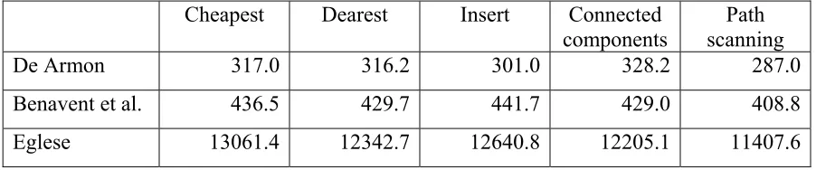
Results from using the five initial solution methods are given in Table 1. The table shows the average solution value over all instances in each set. It will be seen that the quality of these initial solutions is poor compared to the final solutions generated by the TSA.
[Insert Table 1 about here]
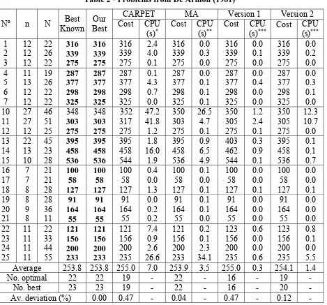
runs of our algorithm that included trials of different swap frequencies. The columns headed “CARPET” give the results reported in Hertz et al (2000). The run times have been divided by 7 to give an approximate comparison between the times on the original computer used by the authors (SGI Indigo2 at 195 MHz) and our algorithm that was coded in C and run using a Pentium Mobile at 1.4 GHz. The columns headed “MA” give the results reported by Lacomme et al (2004), using a Pentium III at 1 GHz. The computing times in their paper have been divided by 1.5 to make them approximately equivalent to the times we recorded for our algorithm. The best results include those reported by Buellens et al. (2003).
[Insert Tables 2, 3 and 4 about here]
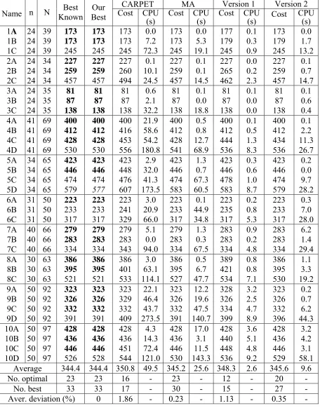
In Tables 2 and 3, if the best known or our best solution is optimal then it is shown in bold. Optimality can be proved for many of the problems in the first two sets using the lower bounding procedures described in Belenguer and Benavent (2003).
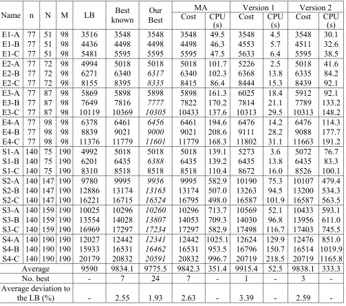
However these lower bounding procedures still leave a gap between the lower bound and the best known solutions for the larger problems in the third set. Recently Ahr (2004) has found improvements to some of these lower bounds and the column LB in Table 4 gives the best lower bounds found so far for these problems. Note that the lower bounds reported for the second set of test problems in Belenguer and Benavent (2003) differ from those reported in Hertz et al. (2000) and Lacomme et al. (2004). This is due to a different cost being used for servicing the required edges. As this is a fixed cost incurred by any solution, the consequence is just that a constant term is needed to adjust the results. Details of the adjustments needed are provided in Belenguer and Benavent (2003).
However in order to properly evaluate the TSA, we should examine the results of Version 1 and Version 2 where the parameters have been fixed. In our computational experiments, we have followed the practice of other researchers by halting the
programme when a known optimal solution has been found. As expected, Version 1 is faster and the average solution over all the instances in each set only exceeds the best known solution or lower bound on the optimal solution (for the third set) by 0.47%, 1.13% and 3.39% respectively for the three problem sets. Version 2 requires longer, but the average solution over all the instances in each set exceeds the best known solution or lower bound on the optimal solution (for the third set) by 0.12%, 0.35% and 2.59% respectively.
Comparison can be made with CARPET for the first two sets of problems. This shows that the average solution values given by CARPET and Version 1 are very similar, but Version 1 is much faster over all the problems. Version 2 gives slightly better
solutions on average than CARPET, finds more best solutions and is still significantly faster.
Comparison can be made with MA for all three sets of problems. Version 1 is much faster than MA, but the results are not quite so good. Version 2 gives results that are very close to those provided by MA. For the first two sets of problems, the computing times for Version 2 are significantly lower than MA. For the final set of problems, the average quality of solution is slightly better for Version 2 and the computing time is lower than required for MA.
5. Conclusions
The paper has demonstrated that the TSA is able to provide high quality solutions to the Capacitated Arc Routing Problem in a reasonable computing time. Several new best solutions are provided for the Eglese set of test problems that have been studied by other researchers.
The results presented demonstrate the good performance of the TSA compared to CARPET and the memetic algorithms approach (MA) of Lacomme et al. (2004). In addition, the TSA is a deterministic algorithm, so all the results are fully reproducible. Both CARPET and MA include several random elements, so different runs of these algorithms may produce different results. CARPET is also complex in the subroutines used within the algorithm. MA is also a complex algorithm and although it has the potential to be easily extended to other problems, it requires many parameters to be set in comparison to the TSA.
The guided local search approach of Beullens et al. (2003) describes an alternative deterministic algorithm for solving the CARP. Their approach also provides high quality solutions in a limited computation time. Their paper reports good results for the DeArmon and the Benavent et al. test problems, but they do not provide any results for the Eglese problems.
References
Ahr D. ,2004. Contributions to Multiple Postmen Problems. Ph.D. Dissertation,
Ruprecht-Karls-Universität, Heidelberg.
Amberg A., Domschke W. and Voss S., 2000. Multiple center capacitated arc routing
problems: A Tabu search algorithm using capacitated trees. European Journal of
Operational Research, 124, 360-376.
Benavent E., Campos V., Corberán E. and Mota E., 1992. The capacitated arc routing
problem. Lower bounds. Networks, 22, 669-690.
Belenguer J.M. and E. Benavent, 2003. A cutting plane algorithm for the capacitated
arc routing problem. Computers and Operations Research, 30(5), 705-728.
Beullens P. Muyldermans L., Cattrysse D. and Van Oudheusden D., 2003. A guided
local search heuristic for the capacitated arc routing problem. European Journal of
Operational Research, 147, 629-643.
Christofides N., 1976. Worst-case analysis of a new heuristic for the traveling salesman problem. Report no. 388, Graduate School of Industrial Administration, Carnegie Mellon University, Pittsburgh.
DeArmon J. S., 1981. A comparison of heuristics for the capacitated Chinese postman problem. Master’s Thesis, University of Maryland, College Park, MD.
Dror M. (ed), Arc Routing. Theory, solutions and applications. Kluwer Academic Publishers, Boston, 2000.
Edmonds J. and E.L. Johnson, 1973. Matching, Euler Tours and the Chinese Postman
Problem. Mathematical Programming 5, 88-124.
Eglese R.W., 1994. Routing winter gritting vehicles. Discrete Appl. Math., 48(3),
231-244.
Eglese R.W. and L.Y.O Li, 1996. A tabu search based heuristic for arc routing with a capacity constraint and time deadline. In: I.H. Osman and J.P. Kelly (eds.),
Metaheuristics: theory and applications, Kluwer, 633-650.
Frederickson G.N., 1979. Approximation algorithms for some postman problems. J. ACM 26 (3), 538-554.
Golden, B.L. and R.T. Wong, 1981. Capacitated arc routing problems. Networks, 11,
305-315.
algorithms for a class of routing problems. Computers and Operations Research, 10(1), 47-59.
Greistorfer P., 2002. A tabu search metaheuristic for the arc routing problem. Preprint submitted to Elsevier Science.
Hertz A., G. Laporte and M. Mittaz, 2000. A Tabu Search Heuristic for the
Capacitated Arc Routing Problem. Operations Research, 48(1), 129-135.
Hertz A. and M. Mittaz, 2001. A variable neighborhood descent algorithm for the
undirected capacitated arc routing problem. Transportation Science, 35(4), 425-434.
Lacomme P., C. Prins and W. Ramdane-Cherif, 2004. Competitive Memetic
Algorithms for Arc Routing Problems. Annals of Operational Research, 131(1-4),
159-185.
Lenstra, J.K. and A.H.G. Rinnooy Kan, 1976. On General Routing Problems.
Networks 6, 273-280.
Li L.Y.O. and R.W.Eglese, 1996. An interactive algorithm for vehicle routing for
winter-gritting. Journal of the Operational Research Society, 47, 217-228.
Pearn W.L., 1989. Approximate solutions for the capacitated arc routing problem.
Computers and Operations Research, 16(6), 589-600.
Pearn W.L., 1991. Augment-insert algorithms for the capacitated arc routing problem,
Computers and Operations Research, 18(2), 189-198.
Pearn W.L. and Wu T.C., 1995. Algorithms for the rural postman problem,
Table 1 – Average solution values from the initial solution methods
Cheapest Dearest Insert Connected
components scanning Path
De Armon 317.0 316.2 301.0 328.2 287.0
Benavent et al. 436.5 429.7 441.7 429.0 408.8
Table 2 - Problems from De Armon (1981)
CARPET MA Version 1 Version 2
Nº n N Known Best Our
Best Cost CPU (s)* Cost CPU (s)** Cost CPU (s)*** Cost CPU (s)***
1 12 22 316 316 316 2.4 316 0.0 316 0.0 316 0.0
2 12 26 339 339 339 4.0 339 0.3 339 0.1 339 0.2
3 12 22 275 275 275 0.1 275 0.0 275 0.0 275 0.0
4 11 19 287 287 287 0.1 287 0.0 287 0.0 287 0.0
5 13 26 377 377 377 4.3 377 0.1 377 0.4 377 0.3
6 12 22 298 298 298 0.7 298 0.1 298 0.0 298 0.1
7 12 22 325 325 325 0.0 325 0.1 325 0.0 325 0.0
10 27 46 348 348 352 47.2 350 26.5 350 1.2 350 12.3
11 27 51 303 303 317 41.8 303 4.7 305 2.4 305 10.7
12 12 25 275 275 275 1.2 275 0.1 275 0.1 275 0.0
13 22 45 395 395 395 1.8 395 0.9 403 0.3 395 0.1
14 13 23 458 458 458 16.0 458 6.5 462 0.9 458 0.1
15 10 28 536 536 544 1.9 536 4.9 544 0.1 536 0.7
16 7 21 100 100 100 0.4 100 0.1 100 0.0 100 0.0
17 7 21 58 58 58 0.0 58 0.0 58 0.0 58 0.0
18 8 28 127 127 127 1.3 127 0.1 127 0.1 127 0.1
19 8 28 91 91 91 0.0 91 0.1 91 0.0 91 0.0
20 9 36 164 164 164 0.2 164 0.1 164 0.0 164 0.0
21 8 11 55 55 55 0.2 55 0.0 55 0.0 55 0.0
22 11 22 121 121 121 7.4 121 0.2 123 0.6 123 0.8
23 11 33 156 156 156 0.9 156 0.1 156 0.0 156 0.1
24 11 44 200 200 200 2.6 200 2.3 200 0.0 200 0.0
25 11 55 233 233 235 26.6 233 34.1 235 0.6 235 5.5
Average 253.8 253.8 255.0 7.0 253.9 3.5 255.0 0.3 254.1 1.4
No. optimal 22 22 19 - 22 - 16 - 19 -
No. best 23 23 19 - 22 - 16 - 20 -
Av. deviation (%) 0.00 0.47 - 0.04 - 0.47 - 0.12 -
* The original value has been divided by 7 (SGI Indigo2 at 195 MHz).
** The original value has been divided by 1.5 (Pentium III at 1 GHz).
*** We used a Pentium Mobile at 1.4 GHz
Table 3 - Problems from Benavent et al. (1992)
CARPET MA Version 1 Version 2
Name n N Known Best Best Our Cost CPU
(s) Cost CPU (s) Cost CPU (s) Cost CPU (s)
1A 24 39 173 173 173 0.0 173 0.0 177 0.1 173 0.0
1B 24 39 173 173 173 7.2 173 5.3 179 0.3 179 1.7
1C 24 39 245 245 245 72.3 245 19.1 245 0.9 245 13.2
2A 24 34 227 227 227 0.1 227 0.1 227 0.0 227 0.1
2B 24 34 259 259 260 10.1 259 0.1 265 0.2 259 0.7
2C 24 34 457 457 494 24.5 457 14.5 462 2.3 457 14.7
3A 24 35 81 81 81 0.6 81 0.1 81 0.1 81 0.1
3B 24 35 87 87 87 2.1 87 0.0 87 0.0 87 0.6
3C 24 35 138 138 138 32.2 138 18.8 138 0.0 138 0.4
4A 41 69 400 400 400 21.9 400 0.5 400 0.1 400 0.1
4B 41 69 412 412 416 58.6 412 0.8 412 0.5 412 2.2
4C 41 69 428 428 453 54.2 428 12.7 444 1.3 434 11.3
4D 41 69 530 530 556 180.8 541 68.9 536 8.3 536 26.7
5A 34 65 423 423 423 2.9 423 1.3 423 0.3 423 0.2
5B 34 65 446 446 448 32.0 446 0.7 446 0.6 446 0.0
5C 34 65 474 474 476 41.3 474 67.3 478 1.0 474 9.7
5D 34 65 579 577 607 173.5 583 60.5 583 8.7 579 28.2
6A 31 50 223 223 223 3.0 223 0.1 223 0.2 223 0.3
6B 31 50 233 233 241 20.9 233 44.9 235 0.8 233 7.0
6C 31 50 317 317 329 66.0 317 34.8 317 5.3 317 28.0
7A 40 66 279 279 279 5.1 279 1.3 283 0.9 283 6.2
7B 40 66 283 283 283 0.0 283 0.3 283 0.2 283 1.4
7C 40 66 334 334 343 94.0 334 67.5 334 4.8 334 29.4
8A 30 63 386 386 386 3.0 386 0.5 389 0.8 386 1.1
8B 30 63 395 395 401 63.1 395 6.7 421 0.8 395 3.3
8C 30 63 521 521 533 114.1 527 47.7 534 7.1 530 19.2
9A 50 92 323 323 323 22.1 323 12.2 328 3.2 323 0.2
9B 50 92 326 326 329 46.4 326 19.6 326 2.5 326 0.7
9C 50 92 332 332 332 43.7 332 47.5 334 4.7 332 6.2
9D 50 92 391 391 409 273.5 391 140.7 399 8.9 396 44.3
10A 50 97 428 428 428 4.3 428 17.0 428 3.6 428 3.2
10B 50 97 436 436 436 14.3 436 3.1 440 5.1 436 4.2
10C 50 97 446 446 451 72.4 446 11.5 448 4.8 446 3.1
10D 50 97 526 528 544 121.0 530 143.3 536 9.2 529 58.1
Average 344.4 344.4 350.8 49.5 345.2 25.6 348.3 2.6 345.6 9.6
No. optimal 23 23 16 - 23 - 12 - 20 -
No. best 33 33 17 - 30 - 15 - 27 -
Aver. deviation (%) 0 1.86 - 0.23 - 1.13 - 0.35 -
Table 4 - Problems from Eglese
MA Version 1 Version 2
Name n N M LB known Best Best Our Cost CPU
(s) Cost CPU (s) Cost CPU (s)
E1-A 77 51 98 3516 3548 3548 3548 49.5 3548 4.5 3548 30.1
E1-B 77 51 98 4436 4498 4498 4498 46.3 4553 5.7 4511 32.6
E1-C 77 51 98 5481 5595 5595 5595 47.5 5633 6.4 5595 38.5
E2-A 77 72 98 4994 5018 5018 5018 101.7 5226 2.5 5018 41.6
E2-B 77 72 98 6271 6340 6317 6340 102.3 6368 13.8 6335 84.2
E2-C 77 72 98 8155 8395 8335 8415 86.4 8444 15.3 8439 92.1
E3-A 77 87 98 5869 5898 5898 5898 161.3 6025 18.4 5912 92.1
E3-B 77 87 98 7649 7816 7777 7822 170.2 7814 21.1 7789 133.2
E3-C 77 87 98 10119 10369 10305 10433 137.6 10313 29.5 10313 148.2
E4-A 77 98 98 6378 6461 6456 6461 194.6 6476 14.2 6476 114.3
E4-B 77 98 98 8839 9021 9000 9021 208.6 9111 28.2 9088 177.7
E4-C 77 98 98 11376 11779 11601 11779 168.3 11802 31.1 11663 191.2
S1-A 140 75 190 4992 5018 5018 5018 139.1 5273 3.6 5072 76.7
S1-B 140 75 190 6201 6435 6388 6435 139.2 6435 13.8 6435 83.3
S1-C 140 75 190 8310 8518 8518 8518 110.4 8672 16.0 8526 100.1
S2-A 140 147 190 9780 9995 9956 9995 582.9 10190 75.3 10107 479.4
S2-B 140 147 190 12886 13174 13165 13174 507.0 13263 94.5 13200 534.3
S2-C 140 147 190 16221 16715 16524 16795 498.0 16587 101.9 16587 563.5
S3-A 140 159 190 10025 10296 10260 10296 713.7 10569 52.1 10433 593.1
S3-B 140 159 190 13554 14028 13807 14053 709.3 14030 96.8 13956 611.0
S3-C 140 159 190 16969 17297 17234 17297 582.9 17498 116.7 17403 745.5
S4-A 140 190 190 12027 12442 12341 12442 1025.1 12624 129.9 12476 851.0
S4-B 140 190 190 15933 16531 16462 16531 953.5 16796 150.7 16514 1019.9
S4-C 140 190 190 20179 20832 20591 20832 996.7 20719 218.5 20719 1165.8
Average 9590 9834.1 9775.5 9842.3 351.4 9915.4 52.5 9838.1 333.3
No. best - 7 24 7 - 1 - 3 -
Average deviation to
the LB (%) - 2.55 1.93 2.63 - 3.39 - 2.59 -