Sede Amministrativa: Università degli Studi di Padova Dipartimento di Fisica e Astronomia Galileo Galilei
Scuola di Dottorato di Ricerca in Fisica Ciclo XXXI
PhD Thesis
Statistical Learning and Inference
at Particle Collider Experiments
PhD School Coordinator: Prof. Franco SimonettoSupervisor: Dott. Tommaso Dorigo
Advances in data analysis techniques may play a decisive role in the discovery reach of particle collider experiments. However, the importing of expertise and methods from other data-centric disciplines such as machine learning and statistics faces significant hurdles, mainly due to the established use of different language and constructs. A large part of this document, also conceived as an introduction to the description of an analysis searching for non-resonant Higgs pair production in data collected by the CMS detector at the Large Hadron Collider (LHC), is therefore devoted to a broad redefinition of the relevant concepts for problems in experimental particle physics. The aim is to better connect these issues with those in other fields of research, so the solutions found can be repurposed.
The formal exploration of the properties of the statistical models at particle col-liders is useful to highlight the main challenges posed by statistical inference in this context: the multi-dimensional nature of the models, which can be studied only in a generative manner via forward simulation of observations, and the effect of nuisance parameters. The first issue can be tackled with likelihood-free inference methods coupled with the use of low-dimensional summary statistics, which may be con-structed either with machine learning techniques or through physically motivated variables (e.g. event reconstruction). The second, i.e. the misspecification of the gen-erative model which is addressed by the inclusion of nuisance parameters, reduces the effectiveness of summary statistics constructed with machine-learning techniques.
A subset of the data analysis techniques formally discussed in the introductory part of the document are also exploited to study the non-resonant production process pp → HH → b¯bb¯b at the LHC in the context of the Standard Model (SM) and its extensions in effective fields theories (EFT), based on anomalous couplings of the Higgs field. Data collected in 2016 by the CMS detector and corresponding to a total of35.9fb−1of proton-proton collisions are used to set an 95% confidence upper limit at 847 fb on the production cross section σ(pp→HH→bbb¯ b¯) in the SM. Upper limits are also obtained for the cross sections corresponding to a representative set
In addition, the exercise of reformulating the goals of high energy physics ana-lysis as a statistical inference problem is combined with modern machine learning technologies to develop a new technique, referred to as inference-aware neural op-timisation. The technique produces summary statistics which directly minimise the expected uncertainty on the parameters of interest, optimally accounting for the ef-fect of nuisance parameters. The application of this technique to a synthetic problem demonstrates that the obtained summary statistics are considerable more effective than those obtained with standard supervised learning methods, when the effect of the nuisance parameters is significant. Assuming its scalability to LHC data scenarios, this technique has ground-breaking potential for analyses dominated by systematic uncertainties.
This document is a summary of the main projects that I have carried out within my PhD in Physics at the University of Padua (UNIPD), between December 2015 and the December 2018. The main research focus, connecting the projects presented here, has been the development and application of new statistical learning techniques in particle collider experiments. Given the interdisciplinary nature of the topics discussed in this thesis, an effort has been made to discuss the research issues and solutions in a domain generic manner, so the links with the fields of statistics and machine learning are more evident. The price of such attempt has likely been a less cohesive narrative, yet I believe that is has been worth the cost for a different take on the data analysis problems at particle colliders.
Most of the work included in this report has been carried out while employed by the INFN - Sezione di Padova as an Early Stage Researcher of the AMVA4NewPhysics MSCA-ITN. AMVA4NewPhysics is a European research network (EU Horizon 2020 Grant Agreement 675440) that provided the funding and context for the ventures described in this document. Part of the results presented here were joint work with other collaborators at CMS experiment at LHC, which is based at the European Organisation for Nuclear Research (CERN).
First and foremost, I would like to thank my PhD supervisor Tommaso Dorigo for his support and guidance during the last three years. In addition to the valuable feedback that he provided on the various projects presented in this document and the much needed help with the seemingly endless bureaucratic endeavours, his advising style was consequential for finding a beneficial balance between exploration of curiosity-driven research ideas and their exploitation. Tommaso is also to blame for many improvements on my writing style as well as the blueprint of a PhD plan including a broad range of training opportunities.
Most of the analysis work within the CMS Collaboration could not have been car-ried out without the help and support of my postdoc officemates Martino Dall’Osso and Andres Tiko, so I would like to thank them both for their work and their friend-ship. The collaboration and discussions with Mia Tosi, Alexandra Oliveira and Roberto Rossin were also instrumental for the CMS analysis work. I would like also to express gratitude towards the other members of the CMS group at Padova, that were very welcoming since the beginning and regularly demonstrated interest and gave feedback on the status of my research. I would also like to acknowledge all assistance received by the administrative staff of the INFN - Sezione di Padova.
A substantial fraction of the work presented here was carried out within the CMS Collaboration, and thus was shaped by interactions with some of its thousands of members by different means including insightful comments after presentations, long e-mail discussions, and the review of diverse documents. In addition to thankfully acknowledge the contributions of all my CMS collaborators, I would like to highlight the role of the members of the CMS Higgs group and the HH subgroup in the de-velopment of the Higgs pair production analysis as well as of Markus Stoye, Mauro Verzetti, Jan Kieseler and Marcel Rieger regarding the project focussed on the in-tegration DeepJet in the CMS software. Some conversations with Sebastien Wertz, Andre David, Gilles Louppe and Joeri Hermans were also particularly relevant to define some aspects of the work presented in this document.
senior members for their effort in organising the various training and collaboration activities, which were important to create an open and productive research envir-onment. Most importantly, I would like to thank the other network students (aka ESRs), which were always available for stimulating chats about research, life or the universe over coffee or beers. I would also like to express my gratitude towards Sabine Hemmer and Pietro Vischia for the energy they devoted to motivate and manage scientific outreach in the form of blogging and Twitter, which turned out to be very positive experiences.
In addition, I would like to thank Giovanna Menardi and Bruno Scarpa from the UNIPD Statisics department for hosting me for one month and providing feedback on the statistical aspects of my research. Maurizio Sanarico at SDG Consulting was also very accommodating during the months spent in Milan. Also to Daniel Whiteson, Peter Sadowski, and other attendants of the ML for HEP meeting in UCI, which gave initial support for the new machine learning technique described in this thesis. I am also thankful to Kostas Vellidis and IASA for hosting me in Athens. The environment provided by CERN both remotely and during the secondment were essential for carrying out the majority of my research so I would like to thank everyone that works to make such institution function as it does.
One achievements are nothing but the product of incremental improvements over the work, ideas and shared experiences of others, thus the present section is guaran-teed to be incomplete. Hence if a conversation we had, a paper you published, a blog post you produced, a presentation you gave, a question you answered, a book you wrote or some open-source software you developed was helpful to the work presented in this thesis, I am sincerely thankful. Last from an academic perspective, I would like to acknowledge Francisco Matorras and Alexander Read for their willingness for their work as external reviewers of this thesis.
At a personal level, moving to Padova was a bit challenging so I am grateful to have been embraced by the Scambio di Lingue group and their Touch Rugby team, through which I met many new friends and provided a great social context in this marvellous city. I would like to thank my family, particularly my parents and my grandparents, for the unconditional love and support they have provided since I happen to remember. Finally, I would like to thank Ksenija, whom I met halfway through this adventure and has been a wonderful companion since, for her persistent encouragement and affection.
Abstract iii
Preface v
Acknowledgements vii
Introduction 1
1 Theory of Fundamental Interactions 5
1.1 The Standard Model . . . 5
1.1.1 Essentials of Quantum Field Theory . . . 8
1.1.2 Quantum Chromodynamics . . . 12
1.1.3 Electroweak Interactions . . . 14
1.1.4 Symmetry Breaking and the Higgs Boson . . . 16
1.2 Beyond the Standard Model . . . 20
1.2.1 Known Limitations . . . 20
1.2.2 Possible Extensions . . . 23
1.3 Phenomenology of Proton Collisions . . . 24
1.3.1 Main Observables . . . 25
1.3.2 Parton Distribution Functions . . . 26
1.3.3 Factorisation and Generation of Hard Processes . . . 28
1.3.4 Hadronization and Parton Showers . . . 29
2 Experiments at Particle Colliders 31 2.1 The Large Hadron Collider . . . 31
2.1.1 Injection and Acceleration Chain . . . 33
2.1.2 Operation Parameters . . . 34
2.1.3 Multiple Hadron Interactions . . . 36
2.1.4 Experiments . . . 38
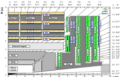
2.2 The Compact Muon Solenoid . . . 39
2.2.2 Magnet . . . 42
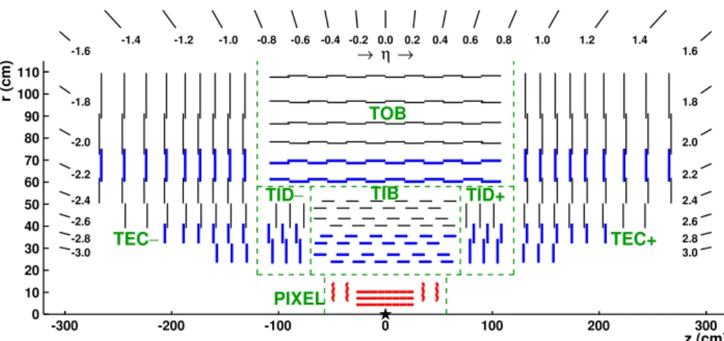
2.2.3 Tracking System . . . 43
2.2.4 Electromagnetic Calorimeter . . . 45
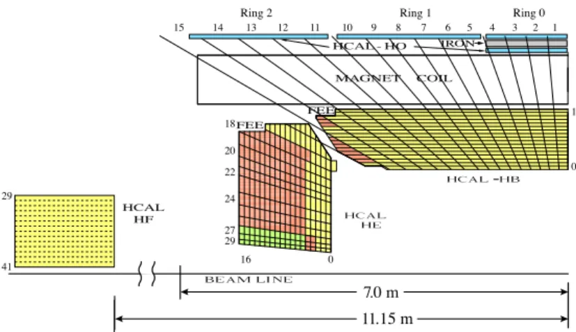
2.2.5 Hadronic Calorimeter . . . 47
2.2.6 Muon System . . . 50
2.2.7 Trigger and Data Acquisition . . . 51
2.3 Event Simulation and Reconstruction . . . 52
2.3.1 A Generative View . . . 53
2.3.2 Detector Simulation . . . 56
2.3.3 Event Reconstruction . . . 58
3 Statistical Modelling and Inference at the LHC 69 3.1 Statistical Modelling . . . 69
3.1.1 Overview . . . 70
3.1.2 Simulation as Generative Modelling . . . 76
3.1.3 Dimensionality Reduction . . . 82 3.1.4 Known Unknowns . . . 92 3.2 Statistical Inference . . . 96 3.2.1 Likelihood-Free Inference . . . 96 3.2.2 Hypothesis Testing . . . 97 3.2.3 Parameter Estimation . . . 102
4 Machine Learning in High-Energy Physics 107 4.1 Problem Description . . . 107
4.1.1 Probabilistic Classification and Regression . . . 108
4.2 Machine Learning Techniques . . . 114
4.2.1 Boosted Decision Trees . . . 115
4.2.2 Artificial Neural Networks . . . 119
4.3 Applications in High Energy Physics . . . 124
4.3.1 Signal vs Background Classification . . . 124
4.3.2 Particle Identification and Regression . . . 129
5 Search for Anomalous Higgs Pair Production with CMS 135 5.1 Introduction . . . 135
5.2 Higgs Pair Production and Anomalous Couplings . . . 137
5.3 Analysis Strategy . . . 139
5.5 Event Selection . . . 144
5.6 Data-Driven Background Estimation . . . 150
5.6.1 Hemisphere Mixing . . . 151
5.6.2 Background Validation . . . 155
5.7 Systematic Uncertainties . . . 164
5.8 Analysis Results . . . 165
5.9 Combination with Other Decay Channels . . . 169
6 Inference-Aware Neural Optimisation 173 6.1 Introduction . . . 174 6.2 Problem Statement . . . 175 6.3 Method . . . 177 6.4 Related Work . . . 181 6.5 Experiments . . . 182 6.5.1 3D Synthetic Mixture . . . 183
7 Conclusions and Prospects 193
Every new beginning
comes from some other beginning’s end.
Seneca the Younger
Humans strive for understanding the world by seeking explanations to the varied natural phenomena happening around them, and accumulating the resulting know-ledge in models that can be used to predict and shape the future reality. The scientific method provides a formal framework for carrying out these investigations and check-ing the validity of the current description of our environment. Recorded experiences of assumed known origin, also known as data, have a central role in updating these explicative theories, because they can provide quantitative or qualitative support to some candidate explanations over others.
Direct sensory perception and personal information processing have a limited in-vestigative reach and are easily affected by subjective conditions. Well understood and calibrated measurement instruments can be used instead for data acquisition, in controlled settings referred to as scientific experiments, so that quantifiability and precision are enhanced. The same applies to theoretical modelling and experimental data analysis, where robust mathematical and computational procedures empower researchers to construct more accurate descriptions of the world we live in. These establish a strong coupling between technology and science, by which technical and conceptual innovations allow the development of better tools, which in turn lead to more scientific knowledge.
The universe is filled with an abundance of interesting phenomena occurring at very different time and space scales, so curious observers might face a difficult choice when deciding what to focus their scientific attention on. Nevertheless, there seems to be a complexity hierarchy whereby larger physical systems are composed by simpler parts, and the properties of the former can be explained by means of those of the latter. Hence, a worthy path of exploration can start with the study of the most fundamental components of nature and their dynamics. At our current level of
understanding, we can reason this would be a quest motivated solely by curiosity, pushed by our desire of making sense of the structure of reality, and not a pragmatic proxy for the development of technological applications. That will be our motivation to delve into experimental particle physics, a discipline dealing with the practical study of the most elementary constituents of matter and their interactions.
The elementary quality of the chosen subject of study does not imply that the jour-ney towards valuable scientific knowledge in this area will be a simple one. On the contrary, as the following chapters will make evident, this undertaking poses grand technical and non-technical challenges which in many cases require novel solutions. Furthermore, the problems at hand are often closely related with those present in other research or technological fields, so their findings and innovations can be repur-posed. Oftentimes this can even be a bidirectional relation, where the obstacles are challenging or original enough that solutions have to go beyond the state of the art in the relevant applied domain. In general, the pursuance of fundamental explanations does require solutions to a multitude of practical problems.
Advances and expertise from other disciplines can accelerate significantly the rate of progress in a fundamental research domain such as experimental particle physics. This is specially relevant in areas such as data analysis, where the infrastructure changes required in evolving environments are low. Yet, some barriers exist against the proliferation of interdisciplinarity, such as field specific language (also known as jargon) and seemingly unclear problem descriptions for collaborators with different backgrounds. This document, in addition to presenting the main research results of the projects I have been involved in the recent past, will attempt to reduce this communication gap by trying to clearly state the main data analysis challenges we face in experimental particle physics in a way they can be linked to other data-centric disciplines such as statistics and machine learning.
The general methodology considered in this work consists on breaking the main research goals in a series of applied problems, express them in a domain-generic way, and understand what is their role in view of the final aim. When possible, the presented concepts and methods will be illustrated with simple use cases when these can help understanding their working principles. The mentioned perspective shift combined with the use of practical but minimal examples has been really useful to identify possible shortcomings on the way data analysis is carried out at the LHC, as well as to develop new techniques capable of addressing them. Nevertheless, we believe that the projects mentioned and presented here are nothing but the first step of what is possible; and the evolution of data analysis techniques and tools could be
a promising route for the advancement of our understanding of the basic building blocks of the universe.
This thesis is organised as follows. Chapter 1provides an overview of our current comprehension of the properties and interactions of the fundamental constituents of nature, followed by a summary of the limitations of our understanding together with the main proposed testable alternative explanations. The links between the mathem-atical description of our universe and the computation of experimental observables will be highlighted when describing the theoretical foundations.
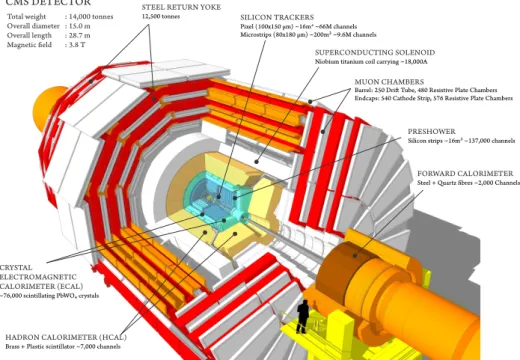
The focus shifts in Chapter2towards how these theories can be experimentally val-idated through scientific experiments. In particular, the discussion revolves around how the design and characteristics of general purpose experiments at high-energy colliders are relevant for the attainment of valuable data that yields new insights on the fundamental properties of the cosmos. The Compact Muon Experiment (CMS) detector at the Large Hadron Collider (LHC) serves as the default example of such an instrument, because it is the scientific experiment that provided the academic context during my graduate (and late undergraduate) years and the main driver of some of the projects included in this report. Experimental modelling and simula-tion will be emphasised in this chapter, due to their importance when extracting knowledge from the acquired data.
Indeed, the problem of obtaining useful information from data is so involved in modern scientific experiments that a standalone chapter will be centered on stat-istical inference concepts and techniques. Inference is the ultimate goal of particle physics experiments, providing a key connection between theory and experiment. In Chapter3we review the problem at hand in particle colliders form a formal statist-ical perspective as well list the main approaches for making quantitative statements based on data and their shortcomings. Two domain-specific aspects of data analysis in high energy physics will be remarked: the generative-only characteristic of accur-ate experimental models and the challenges of dealing with known unknowns we are not interested in, commonly referred as nuisance parameters.
Advancements in computational power coupled with extensive research effort at the intersection between computer science and statistics during the past few decades have contributed to the development of techniques that deal with the automatic improvement of certain objective tasks given some data. An introduction to this family of methods, generally referred to as machine learning techniques, and a review of their usefulness for tackling some common data analysis problem in experimental particle physics, are included in Chapter 4. Some non-trivial connections between
the use of those techniques and the details of the underlying statistical issues will be stressed.
The first four chapters, as outlined above, offer a multi-disciplinary survey of the theoretical and experimental foundations of our understanding of nature and the relevant techniques that allow the extract valuable information from the data. In contrast, Chapter 5 presents a complete example of an analysis at the LHC that applies those techniques to a real-world scenario. Specifically, the use case will be the search for evidence of anomalous non-resonant Higgs boson pair production using CMS data at the LHC, which can be a smoking gun pointing to alternative explan-ations to the current theoretical comprehension of the fundamental interactions and constituents of the universe.
The aforementioned example will be useful to epitomise the main statistical and methodological challenges on the way LHC analyses are carried out. In Chaper 6, we try to shed some light on these issues, and demonstrate how a novel machine learning technique we have developed can deal with one of the most relevant concerns: learning summary statistics using inference-aware losses that account for the effect of nuisance parameters. The limitations of the proposed method as well as alternative solutions to increase the discovery potential of the LHC will be explored.
This document will conclude with Chapter 7, where the main contributions and outcomes of this work will be summarised together with some ideas for future exten-sions and improvements.
1
Interactions
Nothing in life is to be feared. It is only to be understood.
Marie Skłodowska Curie Scientific theories are frameworks describing natural phenomena that are capable of making experimentally testable predictions. Oftentimes, they are specified us-ing mathematical language and built on previous observational knowledge and basic properties of the system under study. At the most fundamental scales known to date, the Standard Model (SM) of particle physics is a scientific theory that provides a very accurate description of most of the observed properties and dynamics of the universe around us. It is constructed upon an innovative theoretical framework, gen-erally referred as quantum field theory (QFT), and principles regarding fundamental symmetries of the laws of nature. In this chapter, a non-exhaustive introduction to this theory and its descriptive reach will be provided together with a summary of the known limitations and possible extensions or alternatives. Given the experimental character of the research discussed in the following chapters, the aim of this chapter is not solely the discussion of the basic structure and properties of the theory, but also the methodology followed to compute predictions for observables that can be contrasted with empirical data.
1.1 The Standard Model
The Standard Model (SM) of particle physics is a mathematically self-consistent gauge field theory that classifies all known types of elementary particles and describes their electromagnetic, weak and strong interactions. Within this fundamental theory, all known matter and energy phenomena can be explained in terms of the kinematics and interactions of elementary particles, which can in turn be understood as local excitations of different fields that permeate our universe.
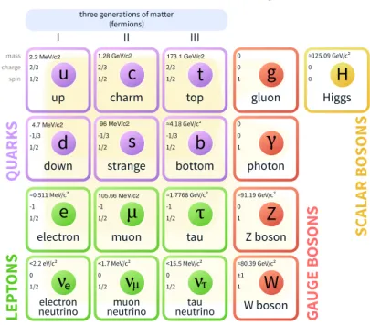
Figure 1.1: Schematic overview of the particle content within the SM. Fundamental particles include fermions, further subdivided in quarks and leptons, and fundamental bosons, including the force mediators and the Higgs boson. Diagram adapted from MissMJ (CC BY 3.0 license).
From a historical perspective, this theory is the product of a succession of import-ant theoretical developments and experimental discoveries over the last century [1], culminating with the discovery of the Higgs boson in 2012 [2,3]. If a more principled viewpoint is taken, the SM can be thought of as the most general but mathematically consistent theory that respects a set of symmetries, namely a global Poincaré group symmetry (translational, rotational and relativistic boost invariance) and a local
GSM=SU(3)C⊗SU(2)L⊗U(1)Y (1.1)
gauge group symmetry. The GSM symmetry group is essential to describe three
of the four fundamental interactions observed in nature: strong interaction, weak interaction and electromagnetic interaction. In fact, the SU(3)C is associated the
strong force and the conservation of its charge, called colour, while the SU(2)L⊗
U(1)Y symmetry instead is related with electroweak interactions (i.e. unification of
weak and electromagnetic) and the conservation of isospin and weak hypercharge. The SM is typically specified using the Lagrangian formalism and depends on a total of 19 parameters (not accounting for neutrino masses and mixing angles), which are not predicted by the theory from first principles, and thus can only be determined through experimental measurements.
In the context of the SM, excitations of the fundamental fields give rise to two types of elementary particles: fermions (characterised by having half-integer spin) and bosons (characterised by having integer spin). Fermions are the fundamental constituents of matter, and they are further subdivided into leptons and quarks depending on their interactions. A schematic overview of the fundamental particles of the SM and their properties is provided in Figure1.1. Three particle generations are known for both quarks and leptons, each containing a pair of particles with different masses. For quarks, the heavier is referred to as up-type and the lighter as down-type. Instead, for leptons we distinguish the heavier charged particles (electron, muon and tau) from their corresponding light and uncharged neutrinos.
Regular matter is largely made of the first generation of quarks and electrons, given that higher generations rapidly decay quickly to lower generations characterised by smaller masses. All fermions interact via the weak force but only quarks carry colour charge and are subjected to the strong force. For each fermion in the SM, there is a another particle with identical properties but opposite quantum numbers, globally referred to as antimatter, and denoted for each particle with the anti prefix and a bar over the symbol (e.g. up antiquarku¯) or by explicitly denoting the charge sign
(e.g. positrone+). Neutrinos are the only fermions that do not carry electrical charge
and might be their own antiparticle.
The mediators of the strong, weak and electromagnetic fundamental interactions are referred to as gauge bosons, and are characterised by having spin 1. To model the strong interaction colour charge exchanges, a total of eight independent strong massless force mediators, or gluons, are needed. Gluons carry colour charge them-selves and thus participate in colour interactions with other gluons, which leads to a phenomenon known ascolour confinement, which will be discussed in Section1.1.2in more detail. The massless and neutralphoton is the mediator of the electromagnetic force, while instead the massive Z,W+ and W− bosons mediate weak interactions. The last piece in the SM is the Higgs boson, the only fundamental known particle with spin 0. The Higgs boson is the quantum excitation of the Higgs field, which also couples with other fundamental particles such as the gauge bosons of the weak force, effectively generating their mass through their interaction. The Higgs boson and Higgs field play an essential role in the electroweak symmetry breaking (EWSB) mechanism, which will be discussed in more detail in Section1.1.4.
The rest of this section will be devoted a more mathematically exhaustive review of the different components of the Standard Model, starting by reviewing the basic formalism of quantum field theories and incrementally building on it do describe the characteristics of both the strong and electroweak interactions that give rise to the diverse interactions dynamics of relevance in particle physics experiments. The mentioned review is heavily inspired by standard bibliographical references on the topic [4,5], and which are recommended directly for a more detailed survey on the subject.
1.1.1 Essentials of Quantum Field Theory
As hinted in the previous section, in quantum field theory (QFT), observed particles are understood as excitations of fields that extend through the whole universe. Quantum field theory unifies the physical foundations of quantum mechanics and special relativity, and can be used to accurately describe phenomena in systems where relativistic and quantum effects are relevant, such as interactions between highly relativistic particles. In QFT, all the known physical processes in the uni-verse are explained in terms of the state and dynamics of a set of fundamental tensor fields. A tensor field can be defined as a continuous and differentiable set of values, such a scalar or a vector, that exist for any given location and time. For simplicity,
the fields in QFT are usually defined in a relativistic coordinate systemx= (t,x)in order treat spacex and timet jointly.
To exemplify the fundamentals of the QFT framework, let us consider the simplest case, e.g. a single field that does not interact with any other field, which will be denoted as ϕ(x). The dynamics of a field (or several fields) in QFT are specified by using the Lagrangian formalism, similarly to what can be done for systems in classical mechanics. However, instead of considering the LagrangianLwhich depends the generalised coordinate vector q(t) and its time derivatives q˙(t), in QFT the Lagrangian density L is commonly used, which depends only on the field ϕ(x) and its first derivative ∂µϕ(x). In an analogous manner to what is done in classical
mechanics to define the action functional Sclassical, we can define the action of the
quantum fieldSQFT as a function of the Lagrangian densityL as follows:
Sclassical=
∫
L(q(t),q˙(t))dt ⇒ SQFT=
∫
L(ϕ, ∂µϕ) d4x (1.2)
noting that the previous definition would also be valid when the Lagrangian depends on multiple fields and their derivatives instead of a single free field. Identically to what is done in classical systems, we can attempt to solve for the field that minimises the action, i.e. δS = 0. With the help of some functional calculus [6], it is possible to obtain the relativistic field theory version of the Euler-Langrange equation:
∂µ ( ∂L ∂(∂µϕ) ) −∂L ∂ϕ = 0 (1.3)
where∂µ =∂/∂xµ and the repetition of the coordinate indexµ∈ {0,1,2,3}means
summation over the product. The previous relation would still apply to each field in the case a Lagrangian including several fields was considered; therefore, given a Lagrangian, we can use Equation 1.3 to obtain their equations of motion. As an example, let us consider the following Lagrangian LDirac, which is a function of a bispinor fieldψ, a 4-dimensional complex vector field that can represent a field whose excitations behave like fermions of massm:
LDirac = ¯ψ(iγµ∂µ−m)ψ (1.4)
whereγµare the gamma matrices andψ¯=ψ†γ0is the spinor adjoint. As the chosen
obtained by minimising the action δS = 0 can be used to obtain field equations of motion that correspond to the Dirac equation [4] for the spinor field and its adjoint:
iγµ∂µψ−mψ= 0 and iγµψ∂¯ µ+mψ¯= 0 (1.5)
as well as the well-known Klein-Gordon equation component-wise(∂µ∂
µ+m2)ψ= 0,
where ∂µ =∂/∂xµ. Both Dirac and Klein-Gordon equations were proposed in the
context of a relativistic formulation of quantum mechanics.
To shed some light on how a field like ψ can represent actual fermions in the universe, such as electrons or positrons, the field can be quantised by considering a plane wave expansion and defining annihilation operators as
p and bsp, as well as
creation asp† and bsp† operators. The field and its adjoint, which can be thought of
directly as operators instead of fields in this context, may then be expressed as:
ψ(x) = ∫ d3p (2π)3 1 √ 2Ep ∑ s ( as pus(p)e−ipx+bsp†us(p)eipx ) (1.6) ¯ ψ(x) = ∫ d3p (2π)3 1 √ 2Ep ∑ s ( bsp¯vs(p)e−ipx+asp†u¯s(p)eipx) (1.7) where us(p) and vs(p) and its adjoints are the free particle solutions of the Dirac
equation,s is their spin andEp their energy. The operators in the previous
quant-isations can be used to define arbitrary many-particle states. The vacuum state|0⟩ can be defined as the state for which as
p|0⟩ =bsp|0⟩= 0. A single free fermion state
of momenta p and spin s can be obtained by applying the creation operators on the vacuum state|p, s⟩=√2Epaps†|0⟩- or alternatively an anti-fermion if the bsp†is
used instead. Multi-particle free states in momenta representation can analogously be defined by the successive application of creation operators over momenta space.
In particle colliders, we are instead interested in interacting theories rather than free theories, given the we aim to compute total and differential cross sections. Inter-acting theories can also be characterised by their Hamiltonian density H=Hfree+
Hint, which can be expressed as a function the Lagrangian density H =πaψ˙a− L,
whereψ˙a is the time derivative of the field andπa is the conjugate momentum. The
Hamiltonian density can divided in Hfree, that is the part corresponding to the free
theory, and Hint that are the additional terms due to interactions. In interacting theories, time-dependence becomes more important and depends only on the Hint component. Additionally, the ground state|Ω⟩can be different in interacting theories from the free theory vacuum state |0⟩.
Let us denote by|i⟩=|ψ(t→ −∞)⟩and|f⟩=|ψ(t→+∞)⟩some arbitrary initial and final multi-particle states, temporarily far before and after the actual interaction being studied happened (i.e. aroundt= 0), respectively. The observables of interest, which are discussed in Section1.3, are a function of the transition amplitude⟨i|S|f⟩
over all possible initial and final states, whereS is an operator describing the trans-ition. The transition probability, which is expressed as the modulus square of the amplitude |⟨i|S|f⟩|2, is therefore also a function of S, fully describing the
time-evolution from the initial the final state. The S operator may be expressed as a perturbative series using the Dyson expansion:
S=T [ exp ( −i ∫ ∞ −∞ d4xHint(x) )] = ∞ ∑ n=0 (−i)n n! ∫ ∞ −∞ d4x 1... ∫ ∞ −∞ d4x nT[Hint(x1)...Hint(xn)] (1.8)
where T is an operator ensuring that the Hamiltonian density factors Hint(xi) are
ordered in time. Each time-ordered term in the series can be written as a sum of normal (i.e. not time ordered) products of permutations using Wicks theorem [7], which can become rather tedious for high orders. The formalism of Feynman diagrams can be used to simplify the computation of observables at a given order in the perturbative expansion.
Based on the previous perturbative series expansion, the transition amplitude ⟨i|S|f⟩can be easily linked with scattering observables when denoted as:
⟨i|S|f⟩=⟨i|1|f⟩+iM(2π)4δ4(∑p i− ∑ pf ) (1.9)
where the first term corresponds to no interaction occurring, and the second includes the matrix elementMincluding all orders in the perturbative orders, and multiplied by a factor making explicit the conservation of momentum between the initial and final state particles. The matrix elementM, which can be computed perturbatively as a function of the momenta of the particles given final state considered, can be used to define the differential cross section:
dσ dΦ ∼ |M| 2 wheredΦ = (2π)4δ4(∑p i− ∑ pf ) ∏ f 1 2Ef d3p f (2π)3 (1.10)
where the proportionality factor is a function of the initial state particles momenta and dΦ is the full phase space differential element for which can be generally
ex-pressed as a product of the final state particle momenta differential elements. Total scattering rates can be obtained by summing over possible initial and final states and integrating over final states. Both differential and total cross sections can be trun-cated at a given perturbative order. The lowest expansion order is referred as leading order (LO), yet considering additional expansion can greatly increase the prediction accuracy so one (NLO) or two (NNLO) orders are often considered, higher orders often being too computationally challenging. A truncation at an additional order
n, relative to the lowest interaction order, will provide corrections proportional to
α=g2/(4π), whereg is the coupling constant characteristic of the interaction.
1.1.2 Quantum Chromodynamics
In a hadron collider such as the LHC, strong interactions between quark and gluons are dominant, and they can be modelled using quantum chromodynamics (QCD). The theory of QCD can be linked to a SU(3) symmetry group and is described by the following gauge invariant Lagrangian density:
LQCD= ¯ψ(γµDµ−mf)ψ− 1 4G a µνGµνa , ψ= ⎡ ⎢ ⎣ ψr ψg ψb ⎤ ⎥ ⎦ (1.11)
where ψ is a spinor quark field for a given flavour f ∈ {u,d,s,c,b,t} and quark mass mf, and each vector component represents a colour degree of freedom.
As-suming that the Gell-Mann matricesλaare used to define a basis for the gluon field
Aµ = 1/2λa∑Aaµ, the covariant derivative can be defined as Dµ = ∂µ−igsAµ,
wheregs is the strong interaction coupling. In turn, the gluon field strength tensor
Ga
µν is also related with the gluon field components:
Ga
µν =∂µAaν −∂νAµa+gsfabcAbµAcν (1.12)
where fabc are the structure constants of the SU(3) gauge group. The last term
accounts for the self-interaction of the gluon, which are the massless and electrically neutral mediators of the strong force. There are two properties of QCD that play an important role from a phenomenological standpoint: confinement andasymptotic
freedom.
The property of confinement has been postulated to explain why isolated quarks and gluons are not found in nature. Quarks have only been found as part of hadrons, that are colour-neutral composite particles. Even though confinement has not been
understood from first principles, because the observables of bound states in QCD at low-energies cannot be computed in a perturbative manner, there exist extensive evidence both from lattice QCD calculations and experiments. In a bound state between quarks, the effective potential includes a term that increases proportional to their distance, so when the quarks are separated by an external energetic interaction, the additional potential energy generates an additional quark-antiquark pair, leading to the formation of bound states. Similar phenomena occur for isolated gluons, which generally are referred as hadronization, and can be understood as a consequence of colour confinement. In particle colliders, successive hadronization and radiation processes led to parton showers (see Section1.3.4).
Quark are then only found in bound states, referred to as hadrons, which can either be mesons or baryons. Mesons are formed by quark-antiquark pairs qq, while¯
baryons are composed of three quarks qqq. Charged and neutral pionsπ+ (u¯d) and
π0 ((uu¯−d¯d)/√2), kaons K+ (u¯s) and K0 (d¯s) and the J/Ψ (c¯c) are among the
most common mesons produced at particle colliders. Baryons instead include the well-known proton (uud) and neutron (udd) that together with electrons are the constituents of most of the known matter in the universe. Many more short-lived baryons exist [8], in addition to the recently discovered exotic bound states referred as tetraquarks [9] and pentaquarks [10]. A detailed description of the compositeness of proton is an essential element for computing LHC observables, as reviewed in Section1.3.2.
Asymptotic freedom is instead linked with the strength reduction of the strong coupling constant when higher energy scales are considered. Let us consider a renor-malisation energy scaleµ2
R, which has to be often defined in order to compute physical
observables which otherwise would be divergent due higher order perturbative cor-rections which cannot be easily calculated. This effect can be also understood as a coupling that varies with the energy scale, which is referred to as a “running” coup-ling constant. The strong force coupcoup-lingαs=gs2/(4π) can thus be approximated as
a function of the renormalisation energy scaleµ2
R as follows: αs(µ2R) = αs(µ20) 1 +αs(µ20) 33−2nf 12π ln (µ2 R µ2 0 ) (1.13)
whereαs(µ20) is the measured coupling at a given energy and nf is total number of
quark flavours which are assumed to be massless in this approximation. The strong interaction thus becomes weaker at higher energies (or short distances) allowing
the perturbative computation of observables related with high-energy interactions, as discussed in Section 1.3. The approximation from Equation 1.13 also provides a lower bound for the energy scale at which QCD can be treated perturbatively, i.e. the denominator becomes zero for an energy scale around200MeV, leading to a diverging coupling constant.
1.1.3 Electroweak Interactions
The remaining two fundamental interactions between elementary particles are the electromagnetic and the weak force. The description of the electromagnetic interac-tion in terms of quantum fields and gauge symmetries, leading to the development of quantum electrodynamics (QED) in the late 1940s, prompted a quest for an ana-logous theory for the weak force. The weak force, known to be responsible for the beta decay at the time, could effectively be modelled using Fermi theory using four-fermion interactions [11] but was not renormalisable and lacked the predictive capabilities and elegance of QED. A large theoretical effort lead to an alternative description based on aSU(2)⊗U(1) symmetry, which unified electromagnetic and weak interactions [12,13], and where the weak interaction was mediated by means of chargedW± and neutralZ massive vector bosons. Nevertheless, the theory did not provide an explanation for the mass of the weak mediators, until the so-called Brout-Englert-Higgs [14,15,16] mechanism for spontaneous symmetry breaking (SSB) was conceived. Higgs also noted explicitly that the mechanism would effectively create an additional scalar field, associated with a new scalar boson, whose existence could experimentally testable. The SSB mechanism was then combined withSU(2)⊗U(1)
unified theory [17] to give rise to what is now known as electroweak theory, which was then proved to be renormalisable [18].
The different testable properties of electroweak phenomena were verified by ex-periments including the existence of weakly-interacting neutral and charged currents [19] and the discovery of the massive W± [20, 21] and Z [22, 23] bosons. Experi-mental evidence also showed that weak interactions were parity violating [24], thus in the electroweak theory the fermion fields are separated in their left-handed ψL
and right-handed ψR chiral components as follows:
ψL =PLψ=
1
2(1−γ5)ψ ψR =PRψ= 1
2(1 +γ5)ψ (1.14)
where PL and PR are the chiral projection operators and γ5 = iγ0γ1γ2γ3 is the
the helicityH = (p·s)/|p| which is the sign of the scalar product of momenta and spin. For massive particles, chirality is still defined but is not identical to helicity which cannot be invariantly defined.
Within the electroweak theory, fermion fields are broken in into their left-handed components, which can be expressed as doublets that would transform underSU(2), and can be denoted as:
Lq = {( u d ) L , ( c s ) L , ( t b ) L } Ll = {( νe e ) L , ( νµ µ ) L , ( µτ τ ) L } (1.15)
and their right handed components, that instead can be expressed as singlets only transforming underU(1):
Ru={uR, cR, tR} Rd={dR, sR, bR} Rl={eR, µR, τR} (1.16)
where the right-handed neutrino components are omitted in the electroweak theory (and the SM), given they are electrically neutral and would not interact weakly when right-handed.
The electroweak interactions then can be made explicit by introducing additional boson fieldsW ={W1, W2, W3} and B which will interact with the fermions.
Sim-ilarly in structure to QED (and also QCD as described in Section 1.1.2), the elec-troweak Lagrangian before spontaneous symmetry breaking is composed by interac-tion terms for the previous doublet and singlet fields, characterised by a covariant derivative, and kinematic terms for both boson fields:
LEW= ψ∈{∑Lq,Ll} ¯ ψ(iγµDµL)ψ+ ψ∈{∑Lq,Ll} ¯ ψ(iγµDRµ)ψ −1 4WµνW µν−1 4BµνB µν (1.17)
where the covariant derivatives for left-handed DLµ and right-handed DRµ fermion fields are respectively defined as:
DLµ=∂µ−1 2gBY Bµ− 1 2gWσWµ DRµ =∂µ−1 2gBY Bµ (1.18)
where σ = {σ1, σ2, σ3} are the Pauli matrices and gB and gW are the coupling
constants. TheWµν andBµν field strength tensors from kinematic terms can in turn
be obtained as:
Wµνi =∂µWνi−∂µWµi−gWϵijkWµiWνk
Bµν =∂µBν−∂µBµ
(1.19)
where ϵijk is the Levi-Civita symbol for each permutation, which is the structure
constant for SU(2).
1.1.4 Symmetry Breaking and the Higgs Boson
The problem with the electroweak theory as described by the Lagrangian from Equa-tion 1.17, which is based on Yang-Mills gauge theory formulation, is that it is not possible to directly add mass term for the fermions nor the weak bosons to the Lag-rangian density without breaking the SU(2)invariance. At the time the mentioned theory was developed, there was extensive evidence not only for lepton masses but also for the weak bosons being massive; the mass required to explain why the weak interaction was short-ranged. The issue of lacking a theoretical mechanism that could explain the mass of fermions and weak boson was solved by the spontaneous symmetry breaking mechanism [14, 15, 16], which is based on postulating the ex-istence of an additional complex scalar field ϕ, which is a SU(2) doublet with the following structure: ϕ= ( ϕ+ ϕ0 ) = ( ϕ3+iϕ4 ϕ1+iϕ2 ) (1.20)
where we made the component notation explicit because it will be relevant later. This scalar field is expected to interact with the electroweak fields W and B by means of the following Lagrangian:
Lscalar = (DHµϕ)†(Dµϕ)−V(ϕ) (1.21)
where the covariant derivate in this case is defined as:
DHµ =∂µ−1
2igBY Bµ− 1
The minimal form for a scalar field potentialV(ϕ), constructed ad-hoc to provide a degenerate vacuum states and a local maximum - a required condition for spontan-eous symmetry breaking, may be expressed as:
V(ϕ) =−µ2ϕ†ϕ+1
2λ(ϕ
†ϕ)2 (1.23)
where both the quadraticµ2 and the quarticλself-interaction parameters are defined
positive with this sign convention. The resulting shape for the potential is often referred as mexican hat, and is depicted in Figure 1.2. The presence of a potential minimum different from the origin gives rises to a non-zero vacuum expectation value for the scalar field:
⟨ϕ⟩0 =
µ2
λ =v
2 (1.24)
whose values depend on the V(ϕ) potential parametersµ2 and λ, and it is denoted
asv2 for convenience. The non-zero vacuum expectation value is thus said to
spon-taneously break the theSU(2)⊗U(1)symmetry, the consequences made more clear when the field is expanded around the minimum:
ϕ= √1 2exp(i σ·G v ) ( 0 v+H ) (1.25)
as a product of a scalar fieldH and a complex exponential of the scalar product of a three-component fieldG={G1, G2, G3} with the Pauli matrices σ ={σ1, σ2, σ3}.
The complex exponential phase can be then removed by aSU(2) group rotation, a transformation that is often referred asunitary gauge. The resulting scalar field can simply be expressed as:
ϕ= √1 2 ( 0 v+H ) (1.26)
where three of the four degrees of freedom in Equation 1.20, which correspond the fieldGwhich would otherwise give rise to the so-called Goldstone bosons, have been removed after the gauge transformation.
Substituting the rotated scalar field from Equation 1.26 in the Lagrangian de-scribed by Equation1.21leads to mass-like terms for linear combinations of the W
and B fields. In order to obtain the physical bosons observed in nature, the mass terms have to be made independent by the following transformations:
Wµ±= √1 2 ( W1 µ∓iWµ2 ) (Zµ Aµ ) = ( cosθW −sinθW sinθW cosθW )( W3 µ Bµ ) (1.27)
where the fieldsW+ andW−are associated with the charged weak bosons, the field
Z with the neutral weak boson, the electromagnetic fieldAwith the photon, andgW
is the Weinberg angle which is related with the electroweak couplings according the relation tanθW =gB/gW. Omitting for now the terms related with the H field, the
Lagrangian in Equation 1.21 leads to the following mass terms for the electroweak force mediators after the unitary gauge and the transformation described in Equation 1.27have been applied:
LEW bosons = 1 2 ( g2 Wv2 4 ) m2 W+ Wµ+W+µ+1 2 ( g2 Wv2 4 ) m2 W− Wµ−W−µ+ 1 2 ( g2 Wv2 4 cosθW ) m2 Z ZµZµ+ 1 2( 0 ) m2 γ AµAµ (1.28)
resulting in mass terms for the massive weak bosons which depend to the weak coupling, the Weinberg angle and the vacuum expectation value of the Higgs field. The last term for the electromagnetic field has only been included to make explicit that no mass term is associated with the electromagnetic force carrierγ. The terms related with the scalarH field (and Higgs boson) are discussed later independently. In addition to providing a mechanism that leads to mass terms for the weak force bosons, additional interactions of the various fermion fields with the scalar field ϕ
can explain their masses. These gauge invariant terms are generally referred to as Yukawa interactions, and correspond to the following Lagrangian terms:
LYukawa=−λl( ¯LlϕRl+ ¯Rlϕ†Ll)
−λd( ¯LqϕRd+ ¯Rdϕ†Lq)
−λu( ¯Lqiσ2ϕ†Ru+ ¯Ruiσ2ϕLq)
(1.29)
where λl , λd and λu are the Yukawa coupling parameters. A charge-conjugate
transformation ϕ → iσ2ϕ† is used to give mass to up-type quarks. For the quark
in the flavour basis, referred to as Cabibbo-Kobayashi-Maskawa (CKM matrix) [25, 26], which can in turn be parametrised by three angles and a complex phase. The fact that the matrix is not diagonal leads to flavour mixing, due to the mass eigen-states being different from flavour eigeneigen-states. Another relevant property of fermion masses is that after spontaneous symmetry breaking, the fermion mass is effectively proportional to its coupling with the Higgs scalar field, which is useful to intuitively understand the dominant interactions and decays of the Higgs boson.
Re(φ)
Im(φ)
V(φ)
A
B
Figure 1.2: Graphical depiction1of the mexican hat potential for the scalar fieldϕ. A local
maximum is present at the origin, but lower energy degenerate minima exist arount it.
In addition of giving masses to both weak bosons and fermions, the remaining degree of freedom after electroweak symmetry breaking gives rise to a scalar field
H. The terms of the Lagrangian concerning only H may be obtained substituting Equation1.26in Equation1.21, leading to the following expression:
LH = 1 2∂µH∂ µH−µ2H2−λvH3−λ 4H 4 (1.30)
where the second (quadratic term) can be interpreted as a scalar boson with a mass
√
2µ2, which is commonly referred as the Higgs boson. A particle with a mass of 125.09(24)GeV [27] and consistent with the expected properties for the Higgs boson was discovered in 2012 by the CMS and ATLAS collaborations [3, 2]. The cubic
λv and quartic λ terms will give rise to self-interaction interaction vertices. The so-called cubic or trilinear Higgs coupling is discussed in a Higgs pair search using data from the CMS experiment in Chapter5. The direct determination of the Higgs
self-coupling is an relevant missing piece, and an important proof of consistency of the spontaneous symmetry breaking mechanism.
1.2 Beyond the Standard Model
The experimental success of the Standard Model and its main subcomponents QED, QCD, and EW unification and symmetry breaking is clearly incontestable, ranging from the confirmation of theoretical prognostication of the existence and some the properties of new particles (e.g.Z,W± and Higgs bosons or top quark) to the agree-ment of precise predictions with meticulous experiagree-mental observations. The fine structure constantα at zero energy scale is an example of the latter, with its exper-imentally determined value consistent among independent physical measurements when the Standard Model based theoretical correction are accounted, down to 12 significant digits [28,29]. In addition to describing natural phenomena with unpre-cedented accuracy, the SM is a self-consistent theory that provides non-divergent predictions at the highest energy scales probed to date.
1.2.1 Known Limitations
In spite of the successes mentioned above, several shortcomings of the Standard Model are known and hence the theory is not considered as a complete theory of natural phenomena at the most fundamental scales. Those concerns include unex-plained empirically observed phenomena such as gravitational interactions, neutrino masses or dark matter particle candidates, theoretical considerations regarding the stability of vacuum or aesthetic principles such as naturalness. Hence, it is presumed that the Standard Model is an effective theory, able to successfully describe funda-mental processes within a range of energies as an approximation of a more complete unified theory. For completeness, the main empirical and theoretical concerns are summarised:
• Omission of gravitational interactions: the current formulation of the SM completely disregards the effect of gravity in fundamental interactions, because no consistent quantum descriptions for gravity matching the experi-mental predictions of the well-established theory of general relativity [30] have been developed to date. While several theoretical efforts are ongoing, such as loop quantum gravity [31] or string theory [32], the coupling for gravitational interactions at the current experimental high-energy reach is expected to be
more than 30 times weaker than for weak interaction, and hence can be safely ignored when computing theoretical predictions.
• Lack of a viable Dark Matter candidate: through a variety of astrophys-ical observations, including the observed galaxy rotation curves [33], gravita-tional lensing [34] and the Cosmic Microwave Background (CMB) [35], there is clear evidence indicating the presence of more gravitational interacting matter in the universe than what is expected by contrasting with the electromag-netic spectra. It has been thus estimated that about 85% of massive existing matter in the universe does not notably interact with ordinary matter and ra-diation, and therefore is referred asDark Matter. While its particular nature is still unknown, scientific consensus seems to favour long-lived cold non-baryonic matter as an explanation, predominantly weakly-interacting massive particles (WIMPs). The three neutrino types are the only WIMP within the Stand-ard Model, but considering the known upper limits on their masses, they can only account for a very small fraction of the total mass of dark matter in the universe.
• Unexplained matter-antimatter asymmetry: as discussed in Section1.1, each matter particle in the Standard Model has an identical anti-matter pos-sessing opposite quantum numbers. Because pair creation and annihilation processes are symmetric, but our universe is manifestly dominated by what we refer as matter, some asymmetric interaction processes ought to exist. Within the SM, some electroweak processes are known to violate CP-symmetry and potentially explain a small part of the observed matter-antimatter asymmetry. New unknown CP-symmetry processes, potentially through interactions not included in the SM, are needed to resolve the mentioned disparity.
• Origin of neutrino masses: the Standard Model was developed assuming that neutrinos were massless, yet is currently well established that neutrinos oscillate between different flavour eigenstates [36, 37], implying that flavour states mix and hence that neutrino masses are very small but different from zero. The SM Lagrangian can be extended to account for the masses of neut-rinos in a similar fashion to what is done for leptons and quarks, but their Yukawa coupling has to be much smaller than of any of the other particles, and it requires the existence of very weakly interacting right-handed neutri-nos. An alternative mechanism for including neutrino masses exists, and it is based on assuming that these particles are Majorana fermions and hence they
are their own anti-particle. This hypothesis is currently being experimentally tested. It also worth noting that in order to explain the smallness of neut-rino masses in a principled way, the Seesaw mechanism [38] has been proposed, which implicitly assumes that the SM is only a low-energy scale effective theory of a more complete unified theory.
• Mismatch between vacuum energy and Dark Energy: in addition of providing evidence for dark matter, astrophysical observations such as studies of the properties of the Cosmic Microwave Background [35] or the redshift of type Ia supernovae [39], consistently point to the hypothesis of an accelerating expansion of the current universe. The simplest way to account for this in cosmological models is to include a cosmological constant, which should be understood as an intrinsic energy density of the vacuum, exerting a negative pressure and therefore driving the observed expansion of the universe. In fact, in order to reconcile the theoretical models with experimental observations, about 68% of the total energy in the present universe would correspond to this type of unknown energy density, generally referred to as Dark Energy. In most quantum field theories, such as the Standard Model, some non-zero zero-point energy originating from quantum fluctuations is expected. However, modern attempts to predict energy densities from QFT are at variance with the observed energy vacuum energy density, some of them differing by 120 orders of magnitude [40].
• Naturalness, hierarchy and fine-tuning concerns: as discussed at the beginning of Section 1.1, the SM can be thought of the most general the-ory based on a set symmetries, and its 19 parameters (or 26 accounting for neutrino masses and mixing angles) are not obtained from first principles but measured experimentally. Having such a large number of free parameters and observing large differences among their relative magnitude has been viewed as a theoretical concern from an aesthetic perspective. A related issue is why the electroweak energy scale (epitomised by the Higgs mass) is much smaller than the assumed cut-off scale of the SM, where gravitational interactions become relevant at MPlanck ≈ 1019GeV, which is generally referred as the hierarchy
problem. In the absence of New Physics or additional interaction mechanisms,
the only way to obtain the observed Higgs mass from the bare Higgs mass (at zero energies) is through a very precise cancellation of divergences, which is regarded as anunnatural or fine-tuned property of the SM theory.
Other possible issues, in some cases related with those discussed, have also been raised. One of them is the apparent vacuum meta-stability [41] and other the so-called strong CP problem [42]. Many of these questions can be clarified once the higher precision measurements of the SM become available, which are mainly ob-tained in particle collider experiments.
1.2.2 Possible Extensions
The known limitations stated in the previous section have motivated the development of alternative theories for describing fundamental interactions. Given the quantitat-ive success of the Standard Model, most of the known proposed theoretical models are either extensions of the SM or its associated predictions can be effectively reduced to those of the SM at the energy range current being explored in particle physics experiments. The set of alternatives that have been proposed is too substantial to be exhaustively listed here, especially given that many of the alternatives include additional free parameters that greatly modify the expected theoretical observables.
Precision Measurements of the SM
Due the existing large space of alternatives to the SM from a theoretical standpoint, the exploration of all possibilities through dedicated searches becomes unattainable. An alternative way to possibly obtain quantitative information pointing to exten-sion of the SM is to measure its most relevant observables with high preciexten-sion. If significant discrepancies are found between the experimental measurement and the theoretical prediction of those observables, it could be evidence pointing to New Physics outside the SM.
Effective Field Theories
In addition to carrying out precision measurements and model-specific searches, there exists a practical way to consider possible extensions due to New Physics phenomena occurring at a higher energy scaleΛthan the one being probed, which will be denoted by E. The model-independent approach often referred to as effective field theory
(EFT) [43,44] allows to compute observables by extending the SM Lagrangian terms from Section1.1with additional operators:
LEFT =LSM+ ∑
i
ci
where Oi are referred to as effective operators, describing the characteristics of the new interactions that are considered in the extended theory and ci are the theEFT
or Wilson coefficients that parametrise the strength of those new interactions. The
integer di defines the dimension of the operator dim(Oi) = [E]di, and while in
prin-ciple an infinite set of operators with any dimension di >4 can be considered, their
effects is expected to be suppressed by (E/Λ)di−4 thus high-dimensional operators
may be neglected when studying the dominant effects of an EFT extension of the SM.
If all the EFT coefficients ci are zero or the new energy scale Λ is infinite, the
EFT theory reduces to the SM Lagrangian. Instead, if Λ≈E, the effective approx-imation in Equation1.31does not hold, and the interactions have to be realistically modelled using a complete theoretical description of the New Physics scenario under study. While in general effective field theories are not renormalisable, observables and higher-order corrections can be computed, because of the well-defined cutoff energy scaleΛ. The best-known example of an EFT that has been used in practice is Fermi theory, which is a useful simplification to compute EW observables at low-energies
E ≈10 MeV rather than an extension of the SM, given that the detailed structure of electroweak interactions due to W± boson mediating β decays was unknown at the time.
At the LHC and other collider experiments, the main use case of EFT is to de-scribe generic extensions of the SM that could arise due to New Physics at energy scales that are not directly accessible. From an experimental standpoint, the goal is thus to constraint the values of the EFT operator coefficients using experimental data. Because the fordi= 5 the only possible operator is relevant for neutrino
phe-nomenology [45], the set of Lagrangian operators of interest at collider experiments often corresponds to di = 6 dimension operators. The large set of possible
dimen-sion six operators can be greatly reduced by requiring that the main experimentally verified properties of the SM are respected, such as the gauge and Poincaré symmet-ries, or baryon number conservation. In Chapter 5, a subset of dimension six EFT operators are used to study non-resonant extensions of Higgs pair production in a model-independent manner.
1.3 Phenomenology of Proton Collisions
Once the properties and limitations of the theoretical model that best describes the current understanding of the fundamental structure and dynamics of nature have
been described, we can delve into how to model proton-proton collisions from a quantitative perspective, so theoretical predictions can be contrasted with experi-mental results at the LHC. The focus of this section then is to make sense of the various outcomes of high-energy proton-proton collisions and how we can predict their relative rates of occurring given some initial state conditions of the interaction.
1.3.1 Main Observables
A related consideration that is useful as an introduction to the aforementioned topic is the question of what outcomes can originate as a result of proton-proton collisions. An answer somehow circular but compatible with our current interpretation of the universe is that everything that could be produced would be produced, meaning that any outcome that can happen in a way that is consistent with the underlying properties of nature is possible. Even though probably the true description of the properties of nature is not known, as discussed in Section 1.1, the Standard Model provides an effective model and restricts considerably the space of possible outcomes, in a way that can be compared with experimental observations. It is worth noting that alternative descriptions of nature, such as those motivated by the known limita-tions of the SM and reviewed in Section1.2, may provide alternative mechanisms for the production of outcomes that are not allowed by the SM, and hence often drive the experimental searches for evidence of New Physics.
For those physical processes that could happen as a product of a proton-proton collision, under the assumption of validity of a particular theoretical model, their total expected rate of occurrence is one the most relevant quantities to predict and compare with observations. To ease its experimental interpretation, the rate of occurrence of any given subnuclear process is commonly expressed as a cross section
σ, which has dimensions of area and is typically expressed in submultiples of barn (1barn= 10−28m2). The advantage of cross sections over rates is that their value is
independent from the density of the incident particle fluxes. The rate, or probability per unit of time, of a process occurring can be computed simply by multiplying its cross section by the instantaneous luminosityLinst, which corresponds to the number of particles per unit of area per unit of time crossing in opposite directions in the collision volume.
Another related concept, which is especially important for simulating interactions, is the differential cross sectiondσ. While the initial state conditions are fixed, the rate of occurrence of a physical process can be expressed as a function of some final-state variables, such as the angle and energy of outgoing particles. While these
variables can be integrated over to compute total cross sections σ, the integrand is proportional to the probability density of each outcome happening as a function of final-state variables, hence its evaluation is crucial for a correct modelling of their multi-dimensional distributions via random sampling. In fact, we will be dealing with differential cross sections instead of total process cross section in this section for generality.
1.3.2 Parton Distribution Functions
A complication that has not been addressed yet is that protons are composite particles, which within a static interpretation can be thought of as the combina-tion of two up-type quarks and one down-type quark bound together via the strong force. The dynamics of proton-proton scattering are then dictated by quantum chro-modynamics (see sec. 1.1.2), which cannot be addressed using perturbation theory for low energies, limiting the first principles computation of relevant observables for the most common interactions. That said, predictions regarding the interaction outcomes from the hard scattering of proton constituents (referred to as partons) can be perturbatively approximated under the assumption of asymptotic freedom at high energies. This allows the modelling of very high energy collisions at particle colliders, which are the focus of most LHC analyses, even if the details about the parton structure cannot be calculated.
When modelling hard (i.e. high energy) scattering processes, a non-perturbative input is required, mainly the probability of finding a particular proton constituent with a certain momentum fraction inside each of the colliding protons, referred to as the parton distribution function (PDF). The model of the proton as three quarks coupled by strong force is too simplistic for modelling proton-proton scattering real-istically, especially at high energies. The continuous exchange of gluons between the three constituent quarks effectively generates a sea of virtual quark-antiquark pairs from which other partons can scatter off. Consequently, in the interaction of two protons, not only the constituent quarks, referred as to valence quarks, can take part in the hard scattering process but also gluons and sea quarks.
At the time of writing, PDFs are not computable from first principles so they have to be parametrised and extrapolated from various experimental sources including fixed-target proton deep inelastic scattering (DIS) and previous collider studies. It is worth noting that the distribution functions depend strongly on the energy scale of the process, yet the evolution for parton densities can be modelled theoretically [47, 48, 49]. Given their relevance for computing observables in high-energy colliders,
x 3 − 10 10−2 10−1 1 0 0.1 0.2 0.3 0.4 0.5 0.6 0.7 0.8 0.9 1 g/10 v u v d d c s u NNPDF3.1 (NNLO) ) 2 =10 GeV 2 µ xf(x, x 3 − 10 10−2 10−1 1 0 0.1 0.2 0.3 0.4 0.5 0.6 0.7 0.8 0.9 1 g/10 v u v d d u s c b ) 2 GeV 4 =10 2 µ xf(x,
(a) Low Energy Scaleµ2= 10GeV2 x 3 − 10 10−2 10−1 1 0 0.1 0.2 0.3 0.4 0.5 0.6 0.7 0.8 0.9 1 g/10 v u v d d c s u NNPDF3.1 (NNLO) ) 2 =10 GeV 2 µ xf(x, x 3 − 10 10−2 10−1 1 0 0.1 0.2 0.3 0.4 0.5 0.6 0.7 0.8 0.9 1 g/10 v u v d d u s c b ) 2 GeV 4 =10 2 µ xf(x,
(b)High Energy Scaleµ2= 104GeV2 Figure 1.3: Distribution functions for the different partons at low and high energies. The
contribution from gluons shown is 1/10 of the actual contribution. Image adap-ted from the NNPDF collaboration [46].
![Figure 1.4: Diagram of a proton-proton collision and the underlying physical processes oc- oc-curring therein, adapted from [52]](https://thumb-us.123doks.com/thumbv2/123dok_us/10182362.2920704/42.892.259.670.341.714/figure-diagram-collision-underlying-physical-processes-curring-adapted.webp)