Abstract—In this work, we developed the concept of super-compression, i.e., compression above the compression standard used. In this context, both compression rates are multiplied. In fact, compression is based on resolution. That is to say, super-compression is a data super-compression technique that superpose spatial image compression on top of bit-per-pixel compression to achieve very high compression ratios. If the compression ratio is very high, then we use a convolutive mask inside decoder that restores the edges, eliminating the blur. Finally, both, the encoder and the complete decoder are implemented on General-Purpose computation on Graphics Processing Units (GPGPU) cards. Specifically, the mentio-ned mask is coded inside texture memory of a GPGPU.
Keywords—General-Purpose computation on Graphics Process- ing Units, Image Compression, Interpolation, Super-resolution.
I. INTRODUCTION
UPERCOMPRESSION represents the most revolutionary con-cept in image and video compression [1]. This concon-cept is based on two simple principles: a) Downsampling/upsampling, i.e., spatial decimation, and b) deblurring, super-resolution, or sharpening [2-6]. While the first was performed using bilinear interpolation, the second we do through a horizontal rafter with a convolution mask, which is based on the Van Cittert’s iterative algorithm [7, 8], and an improvement (non-iterative) that makes the mentioned algorithm computationally more effi-cient, and which was developed by our team [1].
Specifically, the super-compression is a combination of two compressions, i.e., the spatial decimation and the compression of the employed standard. Therefore, the super-compression is a compression above the compression standard used. In this context, both compression rates are multiplied. Super-com-pression is based on super-resolution, because, it increases the compression on the basis of a reduction in size of the image (or frame, in the case of videos) [1].
That is to say, super-compression is a lossy compression technique that superpose spatial image compression on top of bit-per-pixel compression to achieve very high compression ratios. If the compression ratio is very high, then we use a convolutive mask inside decoder that restores the edges, eliminating the blur. Finally, both, the encoder and the Manuscript sent January 11th, 2011.
Mario Mastriani is with the Grupo de Investigación sobre Procesamiento de Señales e Imágenes (GIPSI), Univ. Nac. de Tres de Febrero (UNTreF), 910 Florida St., Floor 6th, Room B, (C1005AAT), CABA, Argentina. phone: +54-11-4015-2295; fax: +54-11-4893-2204; e-mail: [email protected].
te decoder are implemented on General-Purpose computation on Graphics Processing Units (GPGPU) cards. Specifically, the mentioned mask is coded inside texture memory of a GPGPU [1, 9-12].
The Bilinear Interpolation is outlined in Section II, where we discuss the problem of interpolating visually acceptable images at a higher resolution. We first present the interpola-tion problem and why linear interpolainterpola-tion filters are inade-quate for image data. To represent the major mathematical approaches to image processing, we discuss and evaluate five different image interpolation methods. Super-resolution sche-me for compression including linear interpolation are outlined in Section III. Metrics are outlined in Section IV. Simulations are outline in Section V. Finally, Section VI provides a conclu-sion of the paper.
II. BILINEAR INTERPOLATION
Bilinear interpolation is by far the most common interpola-tion method [1-6]. The idea is to interpolate along one dimen-sion using values that were themselves interpolated along the other dimension, see Fig.1.
Fig.1: Bilinear interpolation.
If we have values at (x, y0) and (x, y1), then we could
linearly interpolate along the vertical line. This is not a pro-blem, just generate them by interpolating along the horizontals.
zx0 = (1 − α) z00 + α z10 α = (x − x0)/(x1 − x0)
zx1 = (1 − α) z01 + α z11 (1)
zxy = (1 − β) zx0 + β zx1 β = (y − y0)/(y1 − y0)
Note that it does not matter whether we interpolate across and then down or down and then across (i.e. on x first or y first). Either way we end up with
zxy = (1 − α) (1 − β) z00 + (1 − α) β z01 + α (1 − β) z10 + αβ z11 (2)
Supercompression for Full-HD and 4k-3D (8k)
Digital TV Systems
Mario Mastriani
This is bilinear interpolation. It results in a piecewise func-tion that is not piecewise linear—of course it can’t be, because it matches the data at four different points, and three points uniquely determine the linear function. It has a piece for each cell in the grid of data points, but the interpolation defined over that rectangle is not linear. Look at this most recent equation, remembering that α is a linear function of x and β is a linear function of y. The full expression for zxy is going to
contain a constant term, an x term, a y term, and a xy term. Because of the presence of this last term is not linear.
This kind of function is called bilinear because it is linear as a function of x when y is held fixed and also linear as a function of y when x is held fixed. The quality is obvious, see Fig.2.
Fig.2: Image interpolation using bilinear method of interp2 built-in MATLAB® function. Top: original image. Medium: close-up of
eye in image. Down: interpolated image.
III. SUPER-RESOLUTION SCHEME FOR COMPRESSION This section is organized into four parts, for a better unders-tanding of the concepts:
A. Super-resolution vs Deblurring, B. Compression vs Super-compression, C. Deduction of the mask
D. Applications
A. Super-resolution vs Deblurring:
As we saw in Section I, there is much confusion between the concepts of super-resolution and deblurring in Digital Image Processing [13, 14]. We are going to establish here two rigo-rous definitions for the purpose of eliminating this confusion.
We say that a process is super-resolution if it restores the sharpness of an image involving an increase in the resolution of the same [1-6, 13, 14].
We say that a process is deblurring if it restores the sharp-ness of an image not involving an increase in the resolution of the same. This process is applied when the image sharpness suffers an aberration called blur [13, 14], which comes from a high relative speed of the object in focus in relation to the camera, fast opening and closing the shutter, etc.
We consider important to mention that both processes can involve each other as part of the process of improving the sharpness of the image. In fact, we can understand the super-resolution as a process of increasing the super-resolution followed by a restoration of the edges by a deblurring process. On the other hand, previously established definitions are fundamental to understanding what follows.
B. Compression vs Super-compression:
We define compression as the process reduces the average number of bit-per-pixel (bpp) of an image. In Fig. 3, we repre-sent the set of bit-planes in which decomposes a gray or color image. As seen in Fig. 3, the compression process does not alter the image size [13, 14].
Instead, we define supercompression as the process reduces the average number of bit-per-pixel (bpp) of an image after downsizing. The size reduction process is performed by down-sampling, which takes shrinkage in rows and columns, without obligation to respect the aspect ratio (16:9). In fact, for ISDB-Tb (Integrated Services Digital Broadcasting) Brazilian Digital TV System we use 5:1 as compression rate over the original com-pression of the system, which uses H.264 as video compress-ion standard [15]. When we say, we increase the standard
compression 5 times, this means that we move from a
resolu-tion of 1920x1080 (Full-High Definiresolu-tion: Full-HD) to another 5 times lower of 720x576 (Standard Definition: SD). The standard video compression H.264 is not affected by the supercompression. As discussed in Sub-Section D, supercom-pression requires minimal equipment at the transmitter and the reverse procedure to supercompression in the receiver (set-top-box) [16].
Fig.3: Compression.
However, the unavailability of the latter, the system is compatible, since the receiver will send the SD signal to the Liquid Display Crystal (LCD) TV, which naturally made upsampling obviously changing the aspect ratio, as when a Full-HD LCD TV receive a SD signal. In Fig. 4, we represent the set of bit-planes in which decomposes a gray or color image.
As discussed in Sub-Section D, our supercompression pro-cedure consists in two parts spread in transmitter and receiver.
In transmitter we have three steps: 1. Video slicing: frame-by-frame 2. Downsampling
3. Video reassembling
and in receiver inside set-top-box we have four steps: 1. Receiver of streaming/H.264
2. H.264-1 3. Upsampling 4. Deblurring
In our case, the downsampling and upsampling is done with bilinear interpolation, while the deblurring is done by a bidimen-
Fig.4: Supercompression.
sional convolutive mask of NxN pixels, which makes a rafter over the upsampled (blurred) image. The parameters of this squared mask (where N is odd) are criticals, therefore, the such parameters must be calculated and adjusted with total accu-racy.
In the next section, we will proceed to deduct the mask and set the optimal relationship between its parameters. Later we will proceed to adjust them via trial and error.
C. Deduction of the mask:
Based on the last section, the single frame is recovered after suffering a pair of processes: downsampling and upsampling,
see left side of Fig.5. In this figure:
Xt means original single frame.
Yt means recovered (blurred) single frame.
Mb means square mask of NxN pixels (where N is odd).
This mask is known as a blurred mask, smoothing ope- rator or Point Spread Function (PSF) [2].
↓
means downsampling.↑
means upsampling.Fig.5: Downsampling/upsampling as a blurred mask.
In these processes (
↓
and↑
), the single frame is affected by a space/time invariant blur. On the basis of this, we need an estimator to recover the single frame of the processes affecting it. Then, for an image affected by a downsampling/upsampling as Fig.5, we deduce that the best estimator is the Van Cittert’s recursive algorithm [7, 8].The set of equations reflecting the above model can be divided into two stages: the model and the estimator [1].
Based on Fig.5, we have:
Model: t t
X
X
+1=
(3) t u d tM
X
Y
=
/⊗
(4)Where
⊗
means bidimensional convolution, and Md/urepre-sents a convolutive and unknown mask which summarizes the combined action of downsampling and upsampling together.
Estimator: t t t
X
X
+=
+
λ
×
ε
)
)
1 (5) t t tY
Y
)
−
=
ε
(6) t u d tM
X
Y
)
)
⊗
=
/ (7)Where 0<λ<2 is a constant parameter to adjust. Therefore,
Y
X
0=
)
(8) On the other hand, the computational implementation of the above set of equations involves the use of four nested for’s plus a strict control of the stability of the Eq.5 (with a predictor form) from restricting the possible values of λ, i.e., only it is possible to use 0<λ <2.
Therefore, it is much more efficient to implement such fil-tering through a simple bidimensional mask convolution, eli-minating the predictor form of Eq.5, which allows much more efficient implementations using - for example - a convolution through the Fast Fourier Transform (FFT) [13, 14]. In conse-quence, we need deduce such mask. If we replace Eq.7 in Eq.6, we have, t u d t t
Y
M
X
)
⊗
−
=
/ε
(9) Now, we replace Eq. 9 inside Eq.5, obtaining,(
t d u t)
t tX
Y
M
X
X
)
)
)
⊗
−
×
+
=
+1λ
/ (10)Reagrouping terms of Eq.10, and remembering a model of low noise and linear space and time invariant blur, we have,
t s t
M
Y
X
+1=
⊗
)
(11) Where Ms is a mask as shown in Fig.6, and the followingrela-tionships to consider are very important,
1
)
1
(
N
2−
×
α
+
β
=
, (for deblurring) (12)0
)
1
(
N
2−
×
α
+
β
=
, (for edge detection) (13) Thus, a new and simplified model of deblurring appears on the scene, see Fig.7, where αααα < 0 and ββββ > 1. We need to establish precisely both parameters, then, there are two possi-ble ways forward:1. Choose N (integer, positive, odd and small), and ββββ > 1 (and arbitrarily less than 2), then ααααis derived from Eq.12.
2. Start with arbitrary values of αααα and ββββ (about certain recommendations, e.g., -0.1 < αααα < 0 and 1 < ββββ
≤
2) and generating a random population of the pair [αααα, ββββ], and deducting N from Eq.12.Fig.6: Deblurring mask Ms
The action of this mask can be seen in Fig.8. First, we per-formed an up-scaling of the image, and second, we apply the mask of the Fig.6 on the middle image, thus, obtaining a much higher quality final image [1].
Fig.7: New and simplified model of deblurring.
Fig.8: Our technology with super-resolution
D.Applications:
We present three main applications of video compression in real time for Digital TV, according to standard ISDB-Tb [17].
In the first,we move from a resolution of 1920x1080 Full-HD to another 5 times lower of 720x576 SD. As we have said before, the standard video compression H.264 is not affected by the supercompression.
The Fig.9 shows a diagram of the encoder with three modu-les embedded into GPGPU cards [1, 9-12]. In fact, we work with three GPUs in the encoder.
For starters, the camera delivers pictures with a resolution of 1920x1080 pixels HD-SDI, SDI which means Serial Digital Interface [1].
The first GPU performs a separation of the frames of the video, frame by frame. This procedure is called video slicing [1]. This allows us to individually access each frame to apply downsampling.
The above sampling is conducted in the second GPU, for which, we have selected NVIDIA ® Tesla 2050 [18] for strict customer requirements (see Fig.10), however, can be carried out the same downsampling with a much less powerful, and therefore much less expensive NVIDIA ® GPU, without any problem.
By downsampling, we pass from a resolution of 1920x1080 pixels to another 5 times less, i.e. 720x576. That is to say, from Full-HD to SD. Therefore, we achieve lower bit rate (and therefore the bandwidth used) 5 times.
This seemingly arbitrary compression ratio and reduction of Full-HD format to SD is required by the Argentine govern-ment, so that if a user does not have our decoder, to enjoy the SD broadcast. In this case is the same TV who makes the upsca-
Fig.9: Encoder.
ling, with an obvious change in the original aspect ratio, i.e., from 16:9 to 4:3.
A very important aspect to consider is that this procedure does not require any kind of color transform, i.e., it works directly on the RGB (reed, green and blue) components of each frame. This eliminates the two possible conversions and thus the computational cost they entail.
We used Texture Memory of GPGPU to a computational efficient implementation of the different modules of encoder and decoder, allowing us to reach TV times.
Fig.10 shows in detail the employed technology for the real implementation of Fig.9, which consists in two Quadro GPUs [18] the first for video slicing. frame-by-frame, and the second
Fig.10: Encoder implementation with GPGPUs.
for video reassembling, respectively. The downsampling is im-plemented on a Tesla 250 [18]. However, currently, we have found a way to perform this experiment using only one Quadro GPU. Moreover, in Fig.10:
TX means transmitter
On the other hand, Fig.11 shows a diagram of the decoder implemented inside a set-top-box (STB). So that, if the STB has the superdecompression and depending on the resolution of the LCD TV, we obtain resolutions of High Definition (HD) 720x1280 or Full-HD 1080x1920. However, if the STB hasn’t the superdecompression, the system must be compatible, there-fore we obtain only SD 576x720.
The Fig.12 shows the Super-Resolution Module (SRM) used inside STB of Fig.11, which includes upsampling and deblurring, thus restoring the original resolution.
Fig.11: Decoder.
Fig.13 represents the real implementation of Fig.11, in which, we can see, the set-top-box used in this work, deve-loped by Dixar Inc. [16]. This STB works equally with Terres-trial Digital TV, IPTV, WebTV, 3DTV and Digital Cinema. Besides, this STB has camera and motion sensors, which can be used as interactive gaming platform.
Actually, we are working on an integrated circuit (chip) [19] to replace the current GPGPU inside the STB, minimizing the power consumption and the size of this [16].
Finally, the second application of this technology presented here is shows in Fig.14, where we use a mobile phone with High-Definition Multimedia Interface (HDMI) video out as a receptor.
Fig.12: Super-resolution Module (SRM).
Fig.13: Set-top-box of Dixar Inc.
Fig.14: Mobile phone as HD or Full-HD receptor.
As shows in Fig.14, we take the HDMI video out, and we introduce it in the STB. Depending on the resolution of the LCD TV we obtain HD o Full-HD resolutions.
The original resolution of the mobile phone employed is Low Definition (LD) 320x240 One-Seg (one of 13 segments that form the ISDB-T norm, see Fig.15). In this case, the addi-tional compression rate of STB on H.264 is 27:1 [16].
Finally, the third and last application of this technology presented here is shows in Fig.16 (at the end of this paper), which constitutes the modern Digital TV System 4k-3D desig-ned for Argentine government, which has the same information rate 8k monochannel.
All encoders currently in use (without exception) use intra and interframe compression simultaneously, even modern European coder known as HEVC/H.265 (High Efficiency Video Coding), and which will begin testing in 2013.
The interframe compression is composed of three parts: 1. Scene detection
2. Motion detection
3. Region of Interest (ROI detection)
These three modules are responsible for the delay known as latency, which for European system of digital TV knowed as DVB (Digital Video Broadcasting) is 5.5 seconds, while for the Brazilian system of digital TV knowed as ISDB-Tb system is 4.5 seconds.
If an encoder such as H.264 is used for 3D-4k, thus, the latency would be between 25 and 35 seconds. This is unaccep-table.
At this point, we define latency as the delay between the digital and analog transmission.
On the other hand, H.264 was originally designed for video transmission of low and medium resolution. In fact, for trans-mission for 2k resolution and up, it has shortcomings, morpho-logical defects, and chromatic aberrations. That is to say, it does not fit the 4K-3D, as well as other codecs.
This is the reason that since 2k resolutions can only use intraframe compression, especially the JPEG2000 codec [21, 22].
Since it can not serve interframe compression, then, the compression rates obtained are very low, with the spending disproportionate bandwidth of the channel for transmissions of this type.
Moreover, given that the Argentine government wishes to reuse the digital TV platform installed of Full-HD, then the only viable solution that meets all boundary conditions is one based on supercompression [1].
As shown in Fig.16, we have two images of 3840x2160 pixeles, one for right eye and one for left eye, i.e. a total resolution of 3840 x 2160 x 2 (i.e., stereo). We first performed the downsampling, obtaining two images of 1920x1080 each, which are encoded in H.264 and sent to the transmitter. Once the receiver, upsampling and deblurring is applied to both images, thereby restoring the original resolution.
That is to say, we lower the bit rate of the two images com-bined with a quarter of its value, but, however, both images of 1920x1080 combined occupy about 60% of the bit rate that would occupy the original image transmitted by a system of single-channel Full-HD. This turns out to be a product arising from the characteristics of the method itself [1], which creates a seamless smoothing.
IV. METRICS
A.Data Compression Ratio (CR)
Data compression ratio, also known as compression power,
is a computer-science term used to quantify the reduction in data-representation size produced by a data compression algo-rithm. The data compression ratio is analogous to the physical compression ratio used to measure physical compression of substances, and is defined in the same way, as the ratio bet-ween the uncompressed size and the compressed size [13, 14]:
Size Compressed Size ed Uncompress CR= (14)
Thus a representation that compresses a 10MB file to 2MB has a compression ratio of 10/2 = 5, often notated as an explicit ratio, 5:1 (read "five to one"), or as an implicit ratio, 5X. Note that this formulation applies equally for compres-sion, where the uncompressed size is that of the original; and for decompression, where the uncompressed size is that of the reproduction.
B.Bit-per-pixel (bpp)
The "bits per pixel" refers to the sum of the bits in all three color channels and represents the sum colors available at each pixel before compression (
bc
bpp ). However, as a compression metric, the bits-per-pixel refers to the average of the bits in all three color channels, after of compression process (
ac bpp ). CR bc bpp bc bpp Size ed Uncompress Size Compressed ac bpp = × = (15)
Besides, bpp is also defined as
pixels of Number bits coded of Number ac bpp = (16)
C.Mean Absolute Error (MAE)
The mean absolute error is a quantity used to measure how close forecasts or predictions are to the eventual outcomes. The mean absolute error (MAE) is given by
∑
−∑
= − = − = 1 0 1 0 ) , ( ) , ( 1 NR nr NC nc NRxNC nc nr X nc nr X MAE ) (17)which for two NR×NC (rows-by-columns) monochrome ima-ges X andX
)
, where the second one of the images is conside-red a decompressed approximation of the other of the first one.
D. Mean Squared Error (MSE)
The mean square error or MSE in Image Compression is one of many ways to quantify the difference between an original
image and the true value of the quantity being decom-pressed image, which for two NR×NC (rows-by-columns) monochro-me images X andX
)
, where the second one of the images is considered a decompressed approximation of the other is defined as:
∑
−∑
= − = − = 1 0 1 0 2 ) , ( ) , ( 1 NR nr NC nc NRxNC nc nr X nc nr X MSE ) (18)E.Peak Signal-To-Noise Ratio (PSNR)
The phrase peak signal-to-noise ratio, often abbreviated PSNR, is an engineering term for the ratio between the maximum possible power of a signal and the power of corrupting noise that affects the fidelity of its representation. Because many signals have a very wide dynamic range, PSNR is usually expressed in terms of the logarithmic decibel scale. The PSNR is most commonly used as a measure of quality of reconstruction in image compression, etc [13]. It is most easily defined via the mean squared error (MSE), so, the PSNR is defined as [14]: ) ( 10 log 20 ) 2 ( 10 log 10 MSE X MAX MSE X MAX PSNR= = (19)
Here, MAXX is the maximum pixel value of the image.
When the pixels are represented using 8 bits per sample, this is 256. More generally, when samples are represented using linear pulse code modulation (PCM) with B bits per sample (bps), maximum possible value of MAXX is 2B-1.
For color images with three red-green-blue (RGB) values per pixel, the definition of PSNR is the same except the MSE is the sum over all squared value differences divided by image size and by three [13, 14].
Typical values for the PSNR in lossy image and video compression are between 30 and 50 dB, where higher is better.
V. SIMULATIONS
The simulations are organized in four experiments, separa-ted in two groups: still images (for obvious reasons, however, identical results were achieved in video, HDTV and Digital Cinema) by color and gray. All experiments include calcula-tions of MAE, MSE, PSNR, bpp and CR.
All these experiments involve the comparison between the use of JPEG vs SC (JPEG+SR), and JPEG2000 vs SC (JPEG2000+SR) for still color and gray images, in both cases over a BMP file (which doesn’t have compression, to raw data mode), where the used acronym means:
BMP: BitMap file format [20] JPEG: Joint Picture Group [20]
JPEG2000: JPEG with wavelets [21, 22]
SC: Super-compression SR: Super-resolution
A. Group 1: Main characteristics of employed image:
File = angelina.bmp Color = yes
Size = 1920-by-1080 pixels Original bpp = 24
Experiment 1: JPEG vs SC (JPEG+SR)
JPEG: See Table I, column JPEG, and Fig.17 (2nd from top).
Encoder: 1. From BMP (24 bpp, 1920x1080) 2. To JPEG (0.6853 bpp, 1920x1080) Channel/storage Decoder: 1. From JPEG (0.6853 bpp, 1920x1080) 2. To BMP(24 bpp, 1920x1080)
SC (JPEG+SR): See Table I, column SC (JPEG+SR), and
Fig.17 (3rd from top).
Encoder: 1. BMP (24 bpp, 1920x1080) 2. Downsampling (24 bpp, 720x576) 3. JPEG (0.1445 bpp, 720x576) Channel/storage Decoder: 1. JPEG (0.1445 bpp, 720x576) 2. Upsampling (0.4323 bpp, 1920x1080) 3. Deblurring (0.5004 bpp, 1920x1080) 4. BMP (24 bpp, 1920x1080)
Experiment 2: JPEG2000 vs SC (JPEG2000+SR)
JPEG2000: See Table II, column JPEG2000, and Fig.17 (4th from top). Encoder: 1. From BMP (24 bpp, 1920x1080) 2. To JPEG2000 (2.6285 bpp, 1920x1080) Channel/storage Decoder: 1. From JPEG2000 (2.6285 bpp, 1920x1080) 2. To BMP (24 bpp, 1920x1080)
SC (JPEG2000+SR): See Table II, column SC (JPEG2000+
SR), and Fig.17 (down).
Encoder: 1. BMP (24 bpp, 1920x1080) 2. Downsampling (24 bpp, 720x576) 3. JPEG2000 (0.8148 bpp, 720x576) Channel/storage Decoder: 1. JPEG2000 (0.8148 bpp, 720x576) 2. Upsampling (1.3903 bpp, 1920x1080) 3. Deblurring (2.2397 bpp, 1920x1080) 4. BMP (24 bpp, 1920x1080)
The following tables show the metrics vs the Algorithms for both cases, i.e., JPEG and JPEG2000 vs Supercompression.
TABLE I
ANGELINA (COLOR, 24 BPP, 1920X1080): JPEG VS SC (JPEG+SR)
Metrics JPEG SC (JPEG+SR)
MAE 0.5333 1.0009 MSE 2.3137 7.6264 PSNR 43.6693 38.2393 bpp 0.6853 0.1445 CR 35.0210 166.1154 TABLE II
ANGELINA (COLOR, 24 BPP, 1920X1080): JPEG2000 VS SC (JPEG2000+SR) Metrics JPEG2000 SC (JPEG2000+SR)
MAE 0.0446 0.2961
MSE 0.0472 1.1385
PSNR 61.3884 47.5673
bpp 2.6285 0.8148
CR 9.1307 29.4538
B. Group 2: Main characteristics of employed image:
File = lena.bmp Color = gray
Size = 512-by-512 pixels Original bpp = 8
Experiment 3: JPEG vs SC (JPEG+SR)
JPEG: See Table III, column JPEG, and Fig.18 (2nd from top). Encoder: 1. From BMP (8 bpp, 512x512) 2. To JPEG (0.8953 bpp, 512x512) Channel/storage Decoder: 1. From JPEG (0.8953 bpp, 512x512) 2. To BMP(24 bpp, 512x512)
SC (JPEG+SR): See Table III, column SC (JPEG+SR), and
Fig.18 (3rd from top).
Encoder: 1. BMP (8 bpp, 512x512) 2. Downsampling (8 bpp, 256x256) 3. JPEG (0.2957 bpp, 256x256) Channel/storage Decoder: 1. JPEG (0.2957 bpp, 256x256) 2. Upsampling (0.6502 bpp, 512x512) 3. Deblurring (0.7727 bpp, 512x512) 4. BMP (8 bpp, 512x512)
Experiment 4: JPEG2000 vs SC (JPEG2000+SR)
JPEG2000: See Table IV, column JPEG2000, and Fig.18 (4th from top). Encoder: 1. From BMP (8 bpp, 512x512) 2. To JPEG2000 (3.7242 bpp, 512x512) Channel/storage Decoder: 1. From JPEG2000 (3.7242 bpp, 512x512) 2. To BMP (8 bpp, 512x512)
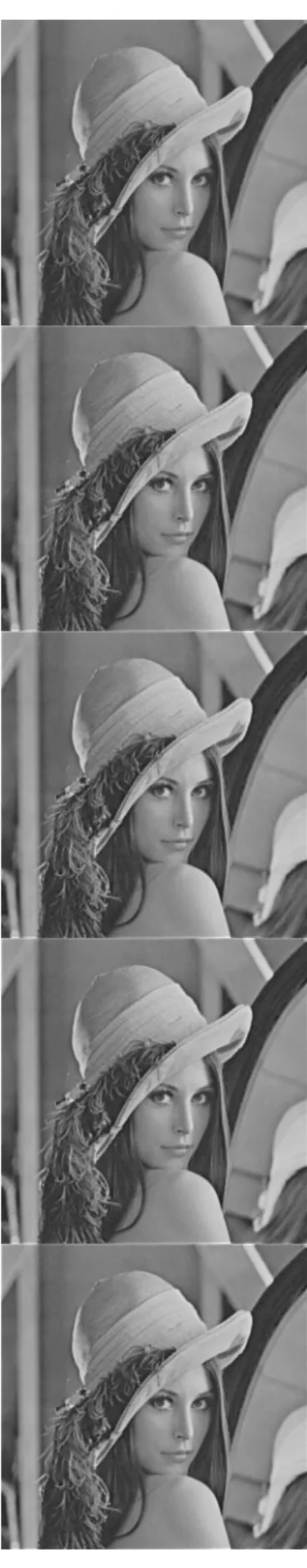
Fig.17: First (top) original image, second (coded and decoded with JPEG), third (coded and decoded with JPEG+Supercompression), fourth (coded and decoded with JPEG2000), fifth (down, coded and
SC (JPEG2000+SR): See Table IV, column SC (JPEG2000+
SR), and Fig.18 (down).
Encoder: 1. BMP (8 bpp, 512x512) 2. Downsampling (8 bpp, 256x256) 3. JPEG2000 (1.0066 bpp, 256x256) Channel/storage Decoder: 1. JPEG2000 (1.0066 bpp, 256x256) 2. Upsampling (1.6421 bpp, 512x512) 3. Deblurring (2.4230 bpp, 512x512) 4. BMP (8 bpp, 512x512)
The following tables show the metrics vs the Algorithms for both cases, i.e., JPEG and JPEG2000 vs Supercompression.
TABLE III
LENA (GRAY, 8 BPP, 512X512): JPEG VS SC (JPEG+SR)
Metrics JPEG SC (JPEG+SR)
MAE 1.0785 2.0243 MSE 4.4363 14.6230 PSNR 41.6606 36.4804 bpp 0.8953 0.2957 CR 8.9358 27.0526 TABLE IV
LENA (GRAY, 8 BPP, 512X512): JPEG2000 VS SC (JPEG2000+SR) Metrics JPEG2000 SC (JPEG2000+SR)
MAE 0.0902 1.5312
MSE 0.0905 9.2596
PSNR 58.5647 38.4649
bpp 3.7242 1.0066
CR 2.1481 7.9475
Finally, all techniques were previously implemented in MATLAB® R2010b (Mathworks, Natick, MA) [23] on a Notebook with Intel® Core(TM) i5 CPU M 430 @ 2.27 GHz and 6 GB RAM on Microsoft® Windows 7© Home Premium 64 bits, and then in NetStream© of Dixar Inc.® [18] on NVIDIA® [18] two Quadro 6000 + Tesla 2050 GPUs for encoder, and NVIDIA® GTX285 GPU inside STB developed by Dixar Inc.® [16] for decoder, as shown in Fig.16.
VI. CONCLUSION
A. Group 1:
Experiment 1: JPEG vs SC (JPEG+SR)
In this experiment SC (JPEG+SR) has MAE, MSE and PSNR with practically the same order of magnitude than JPEG alone, however, bpp is five times lower, at the same time, CR is five times higher, see Table I.
As shown in Fig.17, the second (coded and decoded with JPEG) and the third (coded and decoded with JPEG+Super-compression) from the top, have the same look-and-feel and image quality than the top, i.e., original image of Angelina.
Experiment 2: JPEG2000 vs SC (JPEG2000+SR)
We make similar considerations for this experiment,
regar-Fig.18: First (top) original image, second (coded and decoded with JPEG), third (coded and decoded with JPEG+Supercompression), fourth (coded and decoded with JPEG2000), fifth (down, coded and
ding to the last experiment, see Table II and Fig.17 (fourth coded and decoded with JPEG2000 alone, and fifth coded and decoded with JPEG2000+Supercompression), however, there is a big difference between JPEG and JPEG-2000 to compress this type of image (compare bpp and CR of Table I and II).
B. Group 2:
Experiment 3: JPEG vs SC (JPEG+SR)
In this experiment SC (JPEG+SR) has MAE, MSE and PSNR with practically the same order of magnitude than JPEG alo-ne, however, bpp is five times lower, at the same time, CR is five times higher, see Table III, idem Experiment 1.
As shown in Fig.18, the second (coded and decoded with JPEG) and the third (coded and decoded with JPEG+Super-compression) from the top, have the same look-and-feel and image quality than the top, i.e., original image of Lena.
Experiment 4: JPEG2000 vs SC (JPEG2000+SR)
Identical considerations than Experiment 2 are necessary, see Table IV and Fig.18, with the same conclusions about the difference between JPEG and JPEG-2000 to compress this type of image (compare bpp and CR of Table III and IV).
C. For both groups:
We used Texture Memory inside STB [16] GPGPU to a computational efficient implementation of the bidimensional convolutive mask of deblurring module, allowing us to reach TV times, i.e., a frame every 40 milliseconds.
ACKNOWLEDGMENT
M. Mastriani thanks Prof. Martin Kaufmann, vice chance-llor of Universidad Nacional de Tres de Febrero, for his tre-mendous help and support.
REFERENCES
[1] M. Mastriani, “Single Frame Supercompression of Still Images, Video, High Definition TV and Digital Cinema”, International Journal of Information and Mathematical Sciences, vol. 6:3, pp. 143-159, 2010. [2] A. Gilman, D. G. Bailey, S. R. Marsland, “Interpolation Models for
Image Super-resolution,” in Proc. 4th IEEE International Symposium on Electronic Design, Test & Applications, DELTA 2008, Hong Kong, 2008, pp.55-60.
[3] D. Glassner, S. Bagon, M. Irani. Super-Resolution from a Single Image. Available:
http://www.wisdom.weizmann.ac.il/~vision/single_image_SR/files/singl e_image_SR.pdf
[4] A. Lukin, A. S. Krylov, A. Nasonov. Image Interpolation by
Super-Resolution. Available:
http://graphicon.ru/oldgr/en/publications/text/LukinKrylovNasonov.pdf
[5] Y. Huang, “Wavelet-based image interpolation using multilayer perceptrons,” Neural Comput. & Applic., vol.14, pp.1-10, 2005. [6] N. Mueller, Y. Lu, and M. N. Do. Image interpolation using multiscale
geometric representations. Avalilable:
http://lcav.epfl.ch/~lu/papers/interp_contourlet.pdf
[7] S.H.M. Allon, M.G. Debertrand, and B.T.H.M. Sleutjes, "Fast Deblurring Algorithms", 2004. Available:
http://www.bmi2.bmt.tue.nl/image-analysis/Education/OGO/0504-3.2bDeblur/OGO3.2b_2004_Deblur.pdf
[8] A. Bennia and S.M. Riad, Filtering Capabilities and Convergence of the Van-Cittert Deconvolution Technique, IEEE, Trans. Instrum. Meas., Vol. 41, no. 2, pp. 246-250, Apr. 1992.
[9] M. Kraus, M. Eissele, and M. Strengert. GPU-Based Edge-Directed
Image Interpolation. Available:
http://citeseerx.ist.psu.edu/viewdoc/summary?doi=10.1.1.69.5655
[10] -. NVIDIA CUDA: Best Practices Guide, version 3.0, 2/4/2010. Available:
http://developer.download.nvidia.com/compute/cuda/3_0/toolkit/docs/N VIDIA_CUDA_BestPracticesGuide.pdf
[11] V. Podlozhnyuk. Image Convolution with CUDA, June 2007. Available:
http://developer.download.nvidia.com/compute/cuda/1_1/Website/proje cts/convolutionSeparable/doc/convolutionSeparable.pdf
[12] V. Simek, and R. Rakesh, “GPU Acceleration of 2D-DWT Image Compression in MATLAB with CUDA,” in Proc. Second UKSIM European Symposium on Computer Modeling and Simulations, Liverpool, UK, 2008, pp.274-277.
[13] R.C. Gonzalez, R.E. Woods, Digital Image Processing, 2nd Edition, Prentice- Hall, Jan. 2002, pp.675-683.
[14] A.K. Jain, Fundamentals of Digital Image Processing, Englewood Cliffs, New Jersey, 1989.
[15] I. E. Richardson, H.264 and MPEG-4 Video Compression: Video Coding for Next Generation Multimedia, Ed. Wiley, N.Y., 2003. [16] http://www.dixar.com.ar
[17] http://www.forumsbtvd.org.br/
[18] NVIDIA® (NVIDIA Corporation, Santa Clara, CA).
[19] http://www.untref.edu.ar/carreras_de_grado/ing_computacion.htm
[20] J. Miano, Compressed Image File Formats: JPEG, PNG, GIF, XBM, BMP; Ed. Addison-Wesley, N.Y., 1999.
[21] T. Acharya, and P-S Tsai, JPEG2000 Standard for Image Compression: Concepts, Algorithms and VLSI Architectures, Ed. Wiley, N.Y., 2005. [22] A. Bilgin, and M. W. Marcellin, “JPEG2000 for Digital Cinema” in
Proceedings of 2006 International Symposium on Circuits and Systems (ISCAS), (invited paper), May 2006.
[23] MATLAB® R2010b (Mathworks, Natick, MA).
Mario Mastriani was born in Buenos Aires, Argentina on February 1, 1962. He received the B.Eng. degree in 1989 and the Ph.D. degree in 2006, both in electrical engineering. Besides, he received the second Ph.D. degree in Computer Science in 2009. All degrees from Buenos Aires University. He is Professor of Digital Signal and Image Processing of the Engineering College, at Buenos Aires University (UBA). Professor Mastriani is the Coordinator of Technological Innovation (CIT) of ANSES, and the Computer Engineering Department of the National University of Tres de Febrero, at Buenos Aires, Argentina. He published 51 papers. He is a currently reviewer of IEEE Transactions on Neural Networks, Signal Processing Letters, Transactions on Image Processing, Transactions on Signal Processing, Communications Letters, Transactions on Geoscience and Remote Sensing, Transactions on Medical Imaging, Transactions on Biomedical Engineering, Transactions on Fuzzy Systems, Transactions on Multimedia; Springer-Verlag Journal of Digital Imaging, SPIE Optical Engineering Journal; and Taylor & Francis International Journal of Remote Sensing.
He (M’05) became a member (M) of WASET in 2004.
His areas of interest include Digital Signal Processing, Digital Image Processing, Compression and Super-resolution.