Int. J. Electrochem. Sci., 11 (2016) 7775 – 7784, doi: 10.20964/2016.09.56
International Journal of
ELECTROCHEMICAL
SCIENCE
www.electrochemsci.org
Short Communication
Surface Roughness Influence on CPE Parameters in Electrolytic
Cells
Denner S. Vieira1, Paulo R. G. Fernandes1,2, Hatsumi Mukai1,2, Rafael S. Zola1,3, Giane Gonçalves Lenzi4*, Ervin K. Lenzi5
1
Departamento de Física, Universidade Estadual de Maringá, Avenida Colombo, 5790 – 87020 - 900 Maringá – PR, Brazil
2
National Institute of Science and Technology for Complex Fluids, CNPq, 05508 - 090 São Paulo – SP 3
Departamento de Física, Universidade Tecnológica Federal do Paraná, R. Marcílio Dias, 635 – 86812 - 460 Apucarana – PR, Brazil
4
Departamento de Engenharia Química, Universidade Tecnológica Federal do Paraná, Av Monteiro Lobato, 84016-210 - Ponta Grossa - PR - Brasil
5
Departamento de Física, Universidade Estadual de Ponta Grossa, Av. General Carlos Cavalcanti 4748 – 84030 - 900 Ponta Grossa – PR, Brazil
*
E-mail: [email protected]
Received: 1 June 2016 / Accepted: 18 July 2016 / Published: 7 August 2016
We investigate how the changes on the electrode surface may influence the behavior of the constant– phase elements (CPE) and, consequently, electrical response of an electrolytic cell. This analysis is performed by using an experiment with Milli-Q water and stainless steel electrodes with three different types of polishment: smooth, fine sandpaper, and rough sandpaper. The experimental data is obtained from an Electrical Impedance Spectroscopy (EIS) measure and analyzed by means of an equivalent circuit with CPE elements.
Keywords: Electrical Impedance, CPE, Surface roughness, PNP
1. INTRODUCTION
as a function of the frequency in response to an ac voltage applied, which should have a small amplitude [18]; since a small signal induces tiny perturbations on the system, it will behave linearly [29]. In this context, the solid–liquid interface exhibits all sorts of interesting and important processes [36-37], such as double-layer formation, and adsorption–desorption [1,37].
This rich scenario has motivated the researchers to use different approaches to investigate the electrical response, i.e., the impedance, curves obtained via EIS. For example, at low–frequencies, the experimental data usually reflects surface effects due to the dynamics of the electrolyte particles [29] where the diffusion processes and effects on the surface due to interaction electrode – electrolyte may play a relevant role. In fact, surface effects are important in many situations in condensed matter, entering in contexts that go beyond electro chemistry, such as, the systems studied in references [38,39]. In this scenario, theoretical approaches such as the Poisson–Nernst–Planck (PNP) model [19] and extensions [38] have been used to study some systems that fit into this category [1,40]. Another model used to analyze the EIS data is based on equivalent circuits [12,18,19,29,40] which are usually a useful alternative to interpret the experimental results. In this regard, it is worth to mention equivalent circuits with simple components, such as resistors, capacitors, and inductors are not suitable, in general, to describe the experimental data of an electrolytic cell in all frequency range. This occurs because deviations from the purely capacitive behavior are observed on the EIS data, even when the system is prepared to avoid Faradaic reactions, i.e., absence of charge transfer [41]. In this context, the impedance data is sometimes characterized by 1
i 0 1 and expressed in terms of a constant– phase element (CPE) [16,42]. However, this element in an equivalent circuit, used to model the experimental data, raises important questions concerning the physical meaning of its parameters. Usually the CPE behavior is attributed to the time-constant distributions caused by interfacial heterogeneity although there is not yet a general framework to explain or connect it to more general models [37,38,43-47]. This point leads us to investigate, in an experimental scenario, the influence of the surface roughness on the CPE parameters by analyzing the electrical response obtained from an electrolytic cell with Milli-Q Water. This manner, we intend to have a better comprehension of the effect of the roughness on the electrical response and, consequently, on CPE parameters. To accomplish this, EIS data obtained from an electrolytic cell using electrodes with different surface roughness were used. The details of the experimental procedure are explained in next section, Sec. II. The equivalent circuit used to model the experimental data is discussed in Sec. III. Following our analysis, in Sec. IV, a connection with the PNP model is established. The conclusions of our investigations are presented in the last section of this work, Sec. V.2. THE EXPERIMENT
Fine Sandpaper, 3M Wetordry Sheet 400 Grit Fine Sandpaper, and 3M Sandblaster Power Sanding Sheet 100 Grit Coarse Sandpaper, and named smooth surface, fine surface, and rough surface, respectively, as shown in Fig. 1.
(a) (b) (c)
Figure 1. Surface roughness of the electrodes. The electrodes were submitted to the following process: (a) smooth treatment; (b) fine sandpaper; and (c) rough sandpaper. The images were obtained via optical microscopic using the Leica DM 2500 microscope.
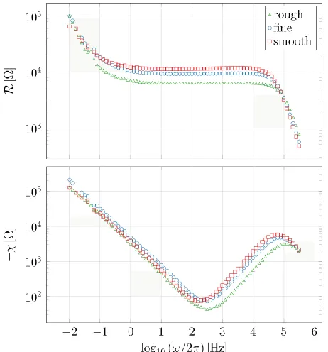
[image:3.596.57.547.148.275.2]To avoid any kind of unwanted substance that could, somehow, affect the EIS data, the electrodes were cleaned with a smooth sponge and neutral detergent and rinsed with Milli-Q water. After they were cleaned a few times, they were left in an ultrasonic bath of acetone (C H O molar mass3 6 58.08gmol1) for ten minutes. To put the electrodes on the sample holder, tweezers were used, to abstain the surfaces of oiliness that could come from the skin. All the measures were made at room temperature. Figure 2 shows the EIS data for the three types of electrodes used.
[image:3.596.184.415.465.713.2]
3. THE MODEL
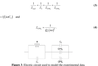
The circuit proposed to analyze the experimental data, obtained with the procedure described in previous section, is shown in the Fig. 3. The first part of the circuit will be used to model the high frequency regime and the second one will be used to model the region of low frequencies, where we expect that the surface effects present on the electrode – electrolyte interface, i.e., the double layer and additional contributions, be relevant. For this circuit, the impedance is given by
Z Z RCZsurf (1)
where the first term corresponds to the RC component of the circuit, is
1
, 1
RC
R i RC
Z (2)
with C1 S d, where is the electric permittivity of the medium,Sthe electrode surface area in contact with the substance, and the distance between the electrodes. The other part of Eq. (1), connected to the surface effects, is written as
1 2
2
1 1 1 1
surf CPE CPE
= + +
Z Z Z Z (3)
where Z2 1
i C 2
and
1k
CPE k Q i
Z . (4)
Figure 3. Electric circuit used to model the experimental data.
[image:4.596.101.500.384.653.2]
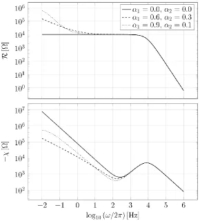
circuit illustrated in Fig. (3) because it is one of the simplest and it can be related to a physico– chemical properties of the system such as diffusion coefficient, number of particles (concentration), and kinetic effects, as we will discuss later on. Some behaviors of equation (1) are illustrated in Fig. (4). This figure shows that the CPE elements play an important role on the circuit’s behavior in low frequency, where the effects between the interface and the electrolyte are expected to be pronounced. The behavior of Eq. (1) in this limit is given by Z~ 1
i with 0 1 where min
1, 2
and it has been reported in several experimental scenarios [9,10,40].4. RESULTS AND DISCUSSION
Figure 4. Electrical impedance of the circuit. Behavior of the real
R Re( )Z
and imaginary
X Im( )Z
parts of the impedance obtained from the circuit illustrated in Fig. 3. The solid black line represents the behavior of the impedance in the absence of the CPE components. The black dashed line represents the circuit with Q12.0 10 61 0.6s and Q21.82 10 61 0.3s . The black dotted line represents the case where Q16.67 10 61 0.9s and6 1 0.1
2 1.11 10
Q s . For simplicity, we have also used R1.0 10 4 and 9
1 2 2.0 10
[image:5.596.155.445.260.584.2]
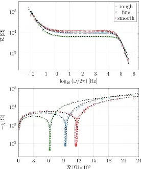
Figure 5 shows the experimental data and the impedance obtained from the model based on the circuit illustrated in Figure 3. We observe a good agreement between the experimental data and the circuit. The parameters were obtained by using the Particle Swarm Optimization (PSO) [48-50] in the fitting process and they are presented in Table 1 (the degree of confidence of the fits is 99.6%). For simplicity, we fixed C1 for all cases present in the first mash of Fig. 3. The other quantities, present in the second mash, were connected to the surfaces effects in the low frequency limit where it is expected the CPEs to play an important role. In this sense, the results presented in Table 1 shows that the different roughness seem to have no relevant influence on the values of and for the cases analyzed. These results, i.e., the good agreement obtained for the three cases with and fixed, allow us to conjecture, for the situation analyzed here, that the effect of the geometry irregularities present in the electrodes is not pronounced on these parameters. Moreover, relevant changes are observed on the parameters Q1 and Q2 which are related to the amplitude of the CPE. We will show in the following, that these parameters can be connected to the adsorption–desorption rates which are related to the Gibbs free energy [51].
Table 1. Parameters from the circuit model. These parameters were obtained from the fitting of the experimental data by the model based on the circuit illustrated in Figure 3. Based on the SI, [R ] = Ω , [C] = F, [Q] = Ω-1sα and α is dimensionless.
Rough Fine Smooth
R [Ω] 6287 9466 11620
C1 [F] 2.12 × 10
-10
2.12 × 10⁻¹⁰ 2.12 × 10⁻¹⁰
C2 [F] 1.98 × 10⁻⁶ 1.61 × 10⁻⁶ 1.46 × 10⁻⁶
α1 0.865 0.865 0.865
α2 0.160 0.160 0.160
Q1 [Ω-1s0.865] 5.70 × 10⁻⁵ 3.95 × 10⁻⁵ 5.74 × 10⁻⁵ Q2 [Ω-1s0.101] 3.72 × 10⁻⁶ 2.50 × 10⁻⁶ 3.02 × 10⁻⁶
In order to obtain more information about the results presented in Table 1, we relate these results with an extension of the PNP model [40]. For this, we consider the limit of low frequencies to evidence the contribution of each element of the circuit presented in Fig. 3 for the system in analysis. In the limit 0 Eq. (1) can be approximated to
1
21
1 2
1 1
2 2 2
1
1 Q Q
R
i C C i C i
Z (5)
and from the extension of the PNP model presented by Lenzi et al. [40], we have
1
2 2
2 1 1
1 PNP
d
i
SD S i
where is the electric permittivity of the medium, S the surface area of the electrode, 2
2
B K T nq
the Debye length, d the distance between the two electrodes (thickness), D the diffusion coefficient, and (i ) is related to the interaction between the electrode – electrolyte, such as mentioned earlier, adsorption – desorption processes. For the present case, we
1 2
1 2
(i ) (i ) (i )
as proposed in Ref. [40].
Table 2. Parameters from the PNP model. Based on the SI, 1 2 1
[ ] F m s , and is dimensionless.
Rough Fine Smooth
κ1 [F-1m2s0.865] 1.53 × 10⁻⁶ 1.60 × 10⁻⁶ 2.85 × 10⁻⁶
η1 0.135 0.135 0.135
κ2 [F-1m2s0.101] 1.00 × 10⁻⁷ 1.01× 10⁻⁷ 1.50 × 10⁻⁷
η2 0.840 0.840 0.840
Figure 5. Real part and Nyquist plot. The experimental data and the model are compared in this figure. The parameters obtained from the agreement between the model and the experimental data for the electrodes with different roughness are shown in Table 1.
[image:7.596.160.436.352.682.2]
2 d R
SD
, 2
2
S C
, k 1 k, (7)
and
2
2 2
k k k
S d
Q
RD
. (8)
The connection between these two models, in the regime of low frequency, shows that the surface effects are directly connected with the CPE elements and that the exponent of these elements are expected to be the same for the all cases, since all the electrodes are made of the same material. Using, D~ 2.0 10 9m s2 1and ~ 76.40which are close from the values of water [52], and the previous relations, we obtain the results reported in Table 2. In particular, they show that 1and 2 depend on the process on the surface, in this case the changes produced on the area of the electrode.
5. CONCLUSION
We have analyzed the electrical response obtained from the Milli-Q water by taking into account electrodes of the same material and surfaces with different characteristics, i.e., geometry irregularities as shown by Figs. 1(a), 1(b), and 1(c). The experimental data, displayed in Fig. 2, indicate that the mechanical treatment used to modify the surface (roughness) of the electrodes influences the electrical response. In particular, we observe that they have different plateaus, implying in different bulk effects. The behavior in the low frequency limit led us to an asymptotic behavior for the impedance, characterized by Z~ 1
i , typical of a CPE element, which is one of the reasons that we took into consideration to model this system by an equivalent circuit with such element. In this sense, it is also interesting to note that the behavior of the real and imaginary parts of the impedance, shown in Fig. 2, seem to be coincident or parallel. This may evidence that the frequency dependence for these quantities is essentially the same. Another concern we had was the connection of the amplitudes, Q1and Q2, and the exponents, 1and 2, present in the constant phase elements with the characteristics and processes exhibited by the system. To treat this matter, a link between the circuit and an extension of the PNP model was proposed. The results obtained from this procedure showed that the constants 1 and 2 manifested different values for different surfaces. In the boundary conditions for the PNP model, these parameters refer to processes on the electrode–electrolyte interface. Considering that the exponents 1 and 2, did not change and the transfer rates 1 and 2 behaved otherwise for the surfaces analyzed here, we are led to conjecture that the contribution of surface geometry irregularities may not be the main point for the CPE exponents.ACKNOWLEDGEMENTS
References
1. M. E. Orazem and B. Tribollet, Electrochemical Impedance Spectroscopy, Wiley (2011). 2. A. Lasia, Electrochemical Impedance Spectroscopy and its Applications, Springer New York
(2014).
3. D. C. Sinclair, T. B. Adams, F. D. Morrison, A. R. West, Appl. Phys. Lett., 80 (2002) 2153–2155. 4. Z. Bao, M. R. Weatherspoon, S. Shian, Y. Cai, P. D. Graham, S. M. Allan, G. Ahmad, M. B.
Dickerson, B. C. Church, Z. Kang, H. W. A. III, C. J. Summers, M. Liu, K. H. Sandhage, Nature 446 (2007), 172–175.
5. E.-C. Shin, P.-A. Ahn, H.-H. Seo, J.-M. Jo, S.-D. Kim, S.-K. Woo, J. H. Yu, J. Mizusaki, J.-S. Lee, Solid State Ionics 232 (2013) 80–96.
6. F. Strubbe, A. R. M. Verschueren, L. J. M. Schlangen, F. Beunis, K. J. Neyts, Colloid Interface Sci., 300 (2006) 396–403.
7. A. Rivera, A. Brodin, A. Pugachev, E. A. J. Rössler, Chem. Phys. 126 (2007) 114503.
8. F. Batalioto, A. R. Duarte, G. Barbero, A. M. F. Neto, J. Phys. Chem. B 114 (2010) 3467–3471. 9. E. K. Lenzi, P. R. G. Fernandes, T. Petrucci, H. Mukai, H. V. Ribeiro, Phys. Rev. E 84 (2011)
041128.
10.F. Ciuchi, A. Mazzulla, N. Scaramuzza, E. K. Lenzi, L. R. Evangelista, J. Phys. Chem. C 116 (2012) 8773–8777.
11.A. R. Duarte, F. Batalioto, G. Barbero, A. M. F. Neto, J. Phys. Chem. B 117 (2013) 2985–2991. 12.D. S. Vieira, M. Menezes, G. Gonçalves, H. Mukai, E. K. Lenzi, N. C. Pereira, P. R. G. Fernandes,
Grasas y Aceites 66 (2015).
13.D. B. Patel, K. R. Chauhan, I. Mukhopadhyay, ChemPhysChem 16 (2015) 1750–1756. 14.O. Josypcuk, K. Holub, V. Marecek, Electrochem. Commun. 56 (2015) 43–45.
15.B. A. Yezer, A. S. Khair, P. J. Sides, D. C. Prieve, J. Colloid Interface Sci. 449 (2015) 2–12. 16.J. R. Macdonald, M. K. Brachman, Rev. Mod. Phys. 28 (1956) 393–422.
17.J. R. Macdonald, Solid State Ionics 13 (1984) 147–149.
18.J. Macdonald, W. Kenan, Impedance Spectroscopy: Emphasizing Solid Materials and Systems, Wiley (1987).
19.E. Barsoukov, J. Macdonald, Impedance Spectroscopy: Theory, Experiment, and Applications, Wiley (2005).
20.S. Grimnes, Bioimpedance and Bioelectricity Basics, Academic Press (2000). 21.E. Katz, I. Willner, Electroanalysis 15 (2003) 913–947.
22.J. Wtorek, A. Polinski, IEEE Trans. Biomed. Eng. 52 (2005) 41–49.
23.A. Schröter, A. Walther, K. Fritzsche, J. Kothe, A. Rosen- Wolff, G. Gerlach, Procedia Chem. 6 (2012) 175–183.
24.R. Kötz, M. Carlen, Electrochimica Acta 45 (2000) 2483–2498. 25.E. Frackowiak, F. Béguin, Carbon 39 (2001) 937–950.
26.E. Frackowiak, F. Béguin, Carbon 40 (2002) 1775–1787.
27.A. Hauch, A. Georg, Electrochimica Acta 46 (2001) 3457–3466.
28.R. Kern, R. Sastrawan, J. Ferber, R. Stangl, J. Luther, Electrochimica Acta 47 (2002) 4213–4225. 29.Q. Wang, J.-E. Moser, M. Grätzel, The Journal of Physical Chemistry B 109 (2005) 14945–14953. 30.M. Jørgensen, K. Norrman, F. C. Krebs, Solar Energy Materials and Solar Cells 92 (2008) 686–
714.
31.B. Liu, H. Muroyama, T. Matsui, K. Tomida, T. Kabata, K. Eguchi, J. Electrochem. Soc. 158 (2011) B215–B224.
32.D. Eder, R. Kramer, Phys. Chem. Chem. Phys. 8 (2006) 4476–4483.
33.M. Fleckenstein, S. Fischer, O. Bohlen, B. Baker, J. Power Sources 223 (2013) 259–267. 34.R. O’Hayre, S. W. Cha, W. Colella, F. B. Prinz, Fuel cell fundamentals, Wiley (2009).
36.S. Baldelli, Accounts of Chemical Research 41 (2008) 421–431.
37.P. Córdoba-Torres, T. J. Mesquita, R. P. Nogueira, The Journal of Physical Chemistry C 119 (2015) 4136–4147.
38.V. G. Guimaraes, H. V. Ribeiro, Q. Li, L. R. Evangelista, E. K. Lenzi, R. S. Zola, Soft Matter, 11 (2015) 1658.
39.R. S. Zola, L. R. Evangelista, Y-C. Yang and D-K. Yang, Physical Review Letters, 110 (2013) 057801.
40.E. K. Lenzi, J. L. de Paula, F. R. G. B. Silva, L. R. Evangelista, J. Phys. Chem. 117 (2013) 23685– 23690.
41.T. Pajkossy, Journal of Electroanalytical Chemistry 364 (1994) 111–125.
42.J. B. Jorcin, M. E. Orazem, N. Pébère, B. Tribollet, Electrochimica Acta 51 (2006) 1473–1479. 43.J. R. Macdonald, The Journal of Physical Chemistry B 113 (2009) 9175–9182.
44.J. R. Macdonald, The Journal of Physical Chemistry C 117 (2013) 23433–23450. 45.C. L. Alexander, B. Tribollet, M. E. Orazem, Electrochimica Acta 173 (2015) 416–424. 46.C. L. Alexander, B. Tribollet, M. E. Orazem, Electrochimica Acta 188 (2016) 566–573. 47.C. L. Alexander, B. Tribollet, M. E. Orazem, Electrochimica Acta (2016).
48.Y. Shi, R. Eberhart, IEEE Computational Intelligence Magazine 98 (1998) 69–73.
49.J. Kennedy, R. Eberhart, IEEE Computational Intelligence Magazine 95 (1995) 1942–1948. 50.R. P. Barbosa, C. H. Martins, L. F. Santos, Acta Scientiarum 34 (2012) 21–25.
51.R. Horne, Water and Aqueous Solutions: Structure, Thermodynamics, and Transport Processes, Wiley-Interscience (1971).
52.R. Robinson, R. Stokes, Electrolyte Solutions: Second Revised Edition, Dover Books on Chemistry, Dover Publications (2002).