Antenna Beam Pattern Modulation with Lattice Reduction Aided Detection

Aided Detection

_.

White Rose Research Online URL for this paper:

http://eprints.whiterose.ac.uk/84535/

Version: Accepted Version

Article:

Ramirez-Gutierrez, R, Zhang, LX and Elmirghani, J (2015) Antenna Beam Pattern

Modulation with Lattice Reduction Aided Detection. IEEE Transactions on Vehicular

Technology, PP (99). ISSN 0018-9545

https://doi.org/10.1109/TVT.2015.2422299

[email protected] https://eprints.whiterose.ac.uk/ Reuse

Unless indicated otherwise, fulltext items are protected by copyright with all rights reserved. The copyright exception in section 29 of the Copyright, Designs and Patents Act 1988 allows the making of a single copy solely for the purpose of non-commercial research or private study within the limits of fair dealing. The publisher or other rights-holder may allow further reproduction and re-use of this version - refer to the White Rose Research Online record for this item. Where records identify the publisher as the copyright holder, users can verify any specific terms of use on the publisher’s website.

Takedown

If you consider content in White Rose Research Online to be in breach of UK law, please notify us by

Antenna Beam Pattern Modulation with Lattice

Reduction Aided Detection

Raymundo Ramirez-Gutierrez, Li Zhang and Jaafar Elmirghani

Abstract

This paper introduces a novel transmission design for antenna beam pattern modulation (ABPM) with

a low complexity decoding method. The concept of ABPM was first presented with the optimal maximum

likelihood (ML) decoding. However, an ML detector may not be viable for practical systems when the

constellation size or the number of antennas is large such as in massive multiple input multiple output

(MIMO) systems. Linear detectors, on the other hand, have lower complexity but inferior performance.

In this paper, we present the antenna pattern selection with a lattice reduction (LR) aided linear detector

for ABPM to reduce the detection complexity with the bit error rate (BER) performance approaching

that of ML while conserving low complexity. Simulation results show that even with this suboptimal

detection, performance gain is achieved by the proposed scheme compared to different spatial modulation

techniques using ML detection. In addition, to validate the results, an upper bound expression for BER

is provided for ABPM with ML detection.

I. INTRODUCTION

Wireless communications are constantly improving, providing an increased data rate, better quality

of service and improved network capacity. Multiple input multiple output (MIMO) has shown extensive

improvements over traditional single antenna systems. The most well known MIMO techniques are

space-time coding (STC) [1] and spatial multiplexing [2] in cases where channel state information (CSI) is not

available at the transmitter.

Submitted toIEEE Trans. Veh. Technol.in March 2014. This work was presented in part at the 2012 International Wireless

Communications and Mobile Computer Conference, Cyprus 2012.

The authors are with the School of Electronic and Electrical Engineering, University of Leeds, Leeds LS2 9JT, United Kingdom

Fig. 1: ABPM system model.

STC aims to improve the reliability of the link which can be achieved by the transmission of multiple

replicas of the same information through independent fading paths [1,2], reducing the probability that

several signals fade at the same time.

Spatial multiplexing improves the spectral efficiency by transmitting multiple independent streams

across multiple antennas. An example of such strategy is the vertical Bell Laboratories layered

space-time (V-BLAST) architecture [3], which requires complex detection and equal or higher number of

antennas at the receiver side compared to the transmitter side. Some hybrid encoding schemes have been

suggested which increase diversity [4] and capacity [5] at the cost of increased computational complexity.

However, diverse constrains have been identified in the implementation of MIMO transmission schemes

that have not been fully investigated [6,7], for instance:

• High inter-channel interference (ICI) is present at the receiver in BLAST transmission systems due

to simultaneous transmissions from multiple antennas.

• The receiver algorithm complexity increases due to the presence of high ICI.

• Performance of BLAST schemes degrades significantly under non-ideal channel conditions [7].

• The above limitations are overcome with full diversity STCs [2,5]. But full-diversity STC systems

(except Alamouti scheme) cannot achieve maximum spectral efficiency of one symbol per symbol

duration. To achieve spectrum efficiency similar to that of BLAST techniques, full-diversity STCs

need to use higher modulation schemes at the cost of reduced reliability.

Transmission techniques based on spatial modulation (SM) [8–12] have been proposed as a solution to

dealing with these issues. They offer a simple design which achieves high data rate. In [13,14], generalized

forms of SM were introduced. In these forms, combinations of antenna indices in addition to conventional

phase spatial shift keying (GPSSK) modulation [14], the results show major improvement in terms of

bit error rate (BER) over generalized space shift keying (GSSK) [12]. This improvement is the result of

transmitting M-ary modulated signals instead of only energy at the position of the selected antennas. In

this way, GPSSK improves spectrum efficiency compared with GSSK and SM without incurring extra

detection complexity.

A beamspace-MIMO which maps phase-shift keying modulated symbols onto orthogonal basis

func-tions on the wavevector domain of the multi-element antenna is proposed in [15–17]. Its performance

is comparable to traditional MIMO systems although only a single active element is used for different

beam patterns.

An antenna beam pattern modulation (ABPM) was proposed by the authors in [18]. ABPM shows a

BER gain when compared to SM techniques employing an ML detector. It exploits the spatial channel

using the antenna pattern to carry information to achieve an efficient information transmission. The

beam pattern is determined by the antenna weights, based on the angle of departure (AoD) from the

transmitter antenna array. All the techniques above use the optimal maximum likelihood (ML) as the

optimal detector at the cost of high computation complexity, especially when the number of antennas

and/or the constellation size are very large, such as in massive MIMO systems.

Linear detection schemes based on the zero forcing (ZF) or the minimum mean square error (MMSE)

criteria are possible solutions [19] for lower complexity detection schemes. However, for ill-conditioned

channels these techniques show an inferior performance compared to the ML detection. The concept of

basis reduction was proposed more than a century ago [20] to find simultaneous rational approximations

to real numbers and to solve the integer linear programming problem in fixed dimensions. The concept

of lattice reduction (LR) is to find a reduced set of basis vectors for a given lattice to obtain certain

properties such as short and nearly orthogonal vectors [20]. For this reason, the LR technique has recently

been exploited to achieve a better conditioned channel matrix by improving its orthogonality conditions

[21–25]. The Lenstra-Lenstra-Lov´asz (LLL) algorithm is widely used in LR to improve the performance

of the linear detectors [26].

This article extends the work done in [18] by proposing optimal antenna pattern selection and reduced

decoding complexity. To reduce the decoding complexity, this article proposes a suboptimal detection

based on the LR technique and derives theoretical analysis for the scheme. The proposed scheme is

evaluated by numerical simulation over independent and identically distributed (i.i.d) Rayleigh fading

channel. The result proves feasible and shows improvements in both reliability and efficiency.

the transmission design, the selection of antenna beam pattern and the sub-optimal detection based on

the LR scheme. Analytic calculation of BER is shown in Section III. Simulation results and comparisons

with other transmission techniques follow in Section IV. The article is concluded in Section V.

Notation: Italicized symbols denote scalar values while bold lower denotes vectors and upper case

symbols matrices. (·)T _and(·)H _{for transpose and conjugate transpose respectively. k · kfor the 2-norm}

of a vector/matrix is used and det(·) indicates the matrix determinant. More notation used: CN(n, σ2)

for the complex Gaussian distribution of a random variable, with mean n and variance σ2. IN denotes

the N×Nidentity matrix andZ is the integer set. O(·) indicates the computational complexity in terms of number of arithmetic operations.

II. ABPM DESCRIPTION

The general ABPM system model consists of a MIMO wireless link betweenNttransmit andNrreceive

antennas. Fig. 1 illustrates the block diagram of ABPM. As shown in the figure, a random sequence of

independent bitsb= [b1 b2 · · · bk]T enters the serial to parallel converter. The firstmbits select an

antenna pattern andk−mbits choose the conventional amplitude/phase modulation (APM) symbols. The

output is mapped to a vectorx= [x1, x2, · · ·, xNt]

T_{. The modulated signal is then transmitted over a}

Nr ×Ntwireless channelH. The received signal is given byy=Hx+v, wherev= [v1 v2 · · · vNr] T

represents the additive white Gaussian noise (AWGN) vector observed at the receive antennas with zero

mean and covariance matrix E[vvH_{] =σ}2

vINr. The channel matrix Hhas i.i.dentries withCN(0,1). The

channel is assumed to be flat-fading, time invariant and independently changing from symbol to symbol.

In our system it is assumed that CSI is available at the transmitter (CSIT), such as in massive MIMO

which is only feasible in reciprocal propagation channels as in time-division duplex (TDD) systems [27].

At the receiver, the antenna patterns and the APM symbol of the signals are estimated by the ABPM

detector, and de-mapped to the transmitted bits.

A. ABPM Transmission

For each symbol period, a stream of independent bits b is sent to the serial to parallel converter and

the output of the converter is divided into two blocks. The first m bits are used to indicate the antenna

pattern which is realised by antenna weight vector denoted asw= [w1, w2, · · · , wNt]

T_{. The second}

part of the symbol will determine the transmitted signalson each antenna. The ABPM transmitted signal

0.2 0.4

0.6 0.8

1

30

210

60

240

90

270 120

300 150

330

180 0

Beam b 1=0 Beam b

1=1

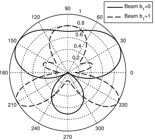
Fig. 2: The two possible beam patterns used in ABPM 2X4 with 3 bits/s/Hz.

The proposed ABPM is capable of transmitting symbols towards different AoDs at the transmitter

side. Antenna patterns are realised by antenna weights, which can be selected to make the best channel

utilisation possible by exploiting the CSIT. In order to facilitate the detection process, it is desirable

for the selected patterns to have minimum correlation between them. The array response vector can be

expressed as a(θ) = [1 e−i2πdsinθλ _{. . . e}−i2π(Nt−1)dsinθ_{λ ]}T_{, where d is the space between antenna}

elements,θindicates the AoD and λis the wavelength [28]. The distance between antenna elements has

to be d≥ λ

2 to avoid correlation.

The weight vectorswshould be obtained to satisfywH[a(θ1) a(θ2) . . . a(θNt)] =wHA= [1, · · ·0,

· · ·1, · · ·0, · · ·0]T_{. Note that, the “1” and “0” in this vector represents the main beam or nulls in}

the radiation pattern, respectively. In the case of where the steering of the main beam is wanted, “1” is

selected. On the other hand, “0” is chosen when the pattern’s nulls are desirable for design purposes. In

this way, the beam patterns can be specified based on CSIT by the angles for the main beam and nulls.

Clearly, as long as the number of independent columns in Ais larger than Nt,w can be solved. So, we

only includedNt columns in A.

As mentioned in [18], the main contribution of this scheme is to use the antenna pattern to transmit

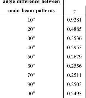
TABLE I: Correlation Table.

angle difference between

main beam patterns γ

10◦ _0.9281

20◦ _0.4885

30◦ _0.3536

40◦ _0.2953

50◦ _0.2679

60◦ _0.2556

70◦ _0.2511

80◦ _0.2503

90◦ _0.2493

TABLE II: Transmission Table of 2-ABPM System.

[b1 b2 b3] Beam s

0 0 0 1 1 + i

0 0 1 1 1 - i

0 1 0 1 -1 - i

0 1 1 1 -1 + i

1 0 0 2 1 + i

1 0 1 2 1 - i

1 1 0 2 -1 - i

1 1 1 2 -1 + i

APM symbols by the selected beam patterns. We define the transmitted vector as[w1·s, w2·s, · · ·, wNt·

s]T _{(i.e. ABPM symbol constellation points). Similar to traditional pulse-amplitude modulation (PAM),}

larger distance between two possible transmitted vectors will result in better performance. For ABPM,

it is possible to maximize the distance between transmit vectors by choosing vectors with minimum

correlation between them. The correlation between antenna beam patterns is denoted as γ with a range

between 1 and 0, indicating completely correlated to no correlation, which is not always possible to

achieve. Table I illustrates the correlation (γ) between two patterns (determined by AoD). A fixed angle

is randomly selected (for simplicity and demonstrative purposes , 0◦ is selected as reference) and the

The 2m _{antenna weight vectors w are combined with the APM symbol (selected by the second}

information block), to generate the transmit vector x which is transmitted over the channel. Thus the

information is carried by both the beam pattern and the APM symbol through the channelH. To clarify

the transmission process an example is given below.

Each ABPM symbol carries 3 bits: two different beam patterns and QPSK modulation. The first block

only has one bit and the second block contains two bits. The mapping table for 3 bits transmission using

QPSK signal modulation and 2x4 MIMO antenna configuration is shown in Table II. The column ‘beam’

in Table II indicates which weight vector is selected at transmission, in other words which antenna beam

pattern is used to transmits. In this example, the beam patterns are: when b1= 0, the angle of the main

beam is at 30◦ _{and the angle of the null is at −30}◦ _{and when b}

1= 1, the angle of the main beam is at −30◦ _{and the angle of the null is at 0}◦_.

Thus, the weight vectors can be calculated by

wH₁ [a(30◦) a(−30◦_{)] =}

 1

0



 wH₂ [a(−30◦_{) a(0}◦_{)] =}

 1

0

 .

Solving the equations the weight vectors are: w1 = [0.5000 + 0.0000i 0.0000−0.5000i]T and

w2 = [0.5000−0.5000i −0.5000 + 0.5000i]T andb2 andb3 are mapped to QPSK symbols according

to Table II.

Fig. 2 shows both antenna beam patterns corresponding tow1 andw2 in the example above. The solid

line shows the pattern corresponding to weight vector w1 in which the main beam is observed at 30◦

and the angle of the null at −30◦_{. The dashed line represents the second pattern which has the main}

beam at −30◦ _{and the angle of the null at 0}◦ _{to increase the directivity of the main lobe, corresponding}

to weight vector w2.

From Table I, it is concluded that the ABPM design for each of the 2m _{patterns should have at least}

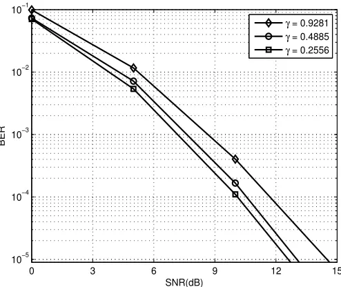
20◦ _{separation in their main lobes to ensure a low correlation. Fig. 3 depicts the BER performance of}

ABPM based on different values ofγ. The three curves are obtained under the same conditions:Nt= 2,

Nr= 4, two beams patterns, QPSK symbols and the spectral efficiency (η) of 3 bits/s/Hz. The detection

used for this figure is based on ML to demonstrate the impact of correlation on the selection of beam

patterns. One of the beams was fixed to 0◦ _{and the second beam was selected based on Table I, to show}

the impact of different correlation values on the ABPM BER performance. The different angles selected

are 60◦_{, 20}◦ _and10◦_{. Each of these angles have a corresponding correlation value:γ = 0.2556, 0.4885}

0 3 6 9 12 15 10−5

10−4 10−3 10−2 10−1

SNR(dB)

BER

γ = 0.9281

γ = 0.4885 γ = 0.2556

Fig. 3: BER versus SNR for cases of using different values of correlation (γ) between antenna beam

patterns, Nt= 2, Nr= 4, two beams patterns.

0.2556), compared to the highly correlated γ = 0.9281. The results above show the correlation impact.

However, in realistic application there are many factors to take into account, e.g. channel conditions,

pattern correlation and ICI mitigation.

B. ML Detection

In [18], as previously stated, ML detection is used. The output of the channel is

y=Hx + v. (1)

The objective of the detector is to estimate the antenna pattern and then de-map them to the information

bits. Assuming all the weight vectors transmitted are equally likely, the optimal detection is given by the

ML method

bj= arg min

j

ky−Hxjk2. (2)

The ML detection ofbj is performed by an exhaustive search across all possible xj for the minimum

The computational complexity of ML is O((NtNr)2L), where Ldenotes the size of the constellation

points [29]. The complexity increases whenLis large, which causes problems when ML based on ABPM

is applied. Linear detectors such as zero-forcing (ZF) and minimum mean-square error (MMSE) are good

solutions with low complexity. However, their BER performance is far worse than ML.

The ZF equaliser removes all inter-symbol interference (ISI), and is ideal when the channel is noiseless.

However, when the channel is noisy, the ZF equaliser will amplify the noise greatly in the attempt to

invert the channel completely. The MMSE equaliser, on the other hand, does not usually eliminate ISI

completely but instead minimizes the total power of the noise and ISI components in the output.

C. Lattice Reduction

Recently, LR aided detectors have been used for MIMO systems to achieve performance with full

diversity and low complexity. [22,23,30,31] show the results of LR improvements over linear detectors

with only a small increase in complexity. Lattice is a set of discrete points representing integer linear

combinations of linearly independent vectors, which are called basis. Given n linearly independent

vectorsc1,c2, ...,cn∈R, the lattice generated by them is defined asL(c1,c2, ...,cn) ={Σni=1sici|si∈Z}.

c1,c2, ...,cn are referred to as the basis of the lattice [32].

A lattice can be represented by many different basis. The main purpose of lattice reduction is to find

a good basis for a given lattice. A basis is considered to be good when the basis vectors are close to

orthogonal. Recently, these LR aided linear equalisers have been utilised for detection in MIMO systems.

Taking the model in (1), x ∈ Z, Hx forms a lattice spanned by the columns of H [33]. Therefore, the estimate of x (based on the received signal y) is the point on the lattice that is closest to y. High

estimation accuracy is achieved when the lattice basis is orthogonal or close to that. This does not affect

the performance of the ML detector, since it performs the same without taking the channel conditions

into account. However, when the ML detector is not used, the channel conditions are important and in

consequence when this condition (orthogonality between lattice vectors) is not satisfied, the performance

tends to degrade. To quantify the orthogonality of a matrix, the orthogonality deficiency (od) [34] for a

matrix His defined as

od(H_{)= 1−} det(H

H_H)

QNt

n=1khnk,

(3)

where hn is the nth column of the matrix H. It is important to note that 0≤od(H)≤1. If od(H) = 1, H

is singular and when od(H) = 0 all the columns of Hare orthogonal. Generally, it is not possible to get

Therefore, if the matrixH˜ represents a new basis for the same lattice spanned by the columns inHand

is more orthogonal thanH, it is anticipated that the performance using linear equalisers should be closer

to the performance of the ML detector. The new channel matrixH˜ is obtained by the LR technique. Arjen

Lenstra, Hendrik Lenstra and Laszlo Lov´asz introduced the LLL algorithm, as a polynomial-time lattice

reduction. It was proposed in 1982 and has since then been used in fields such as computer algebra,

cryptology and algorithmic number theory [35]. The original applications of LLL algorithm were to give

polynomial time algorithms for factorizing polynomials, to find simultaneous rational approximations to

real numbers and to solve the integer linear programming problem in fixed dimensions. The LLL is the

most popular algorithm used in LR aided detectors because in spite of not guaranteeing that the optimal

basis will be found, it guarantees finding a basis with a better value of od. The highest complexity in

terms of number of arithmetic operations in attempting to find a new basis using the LLL algorithm is

O(R4_{), whereRis the size of the basis [24]. In [24], the detailed LLL algorithm using MATLAB notation}

is given. δ is the parameter which controls the performance and complexity of the LLL algorithm, it is

randomly selected from (1₂,1), to guarantee a firm basis reduction. However, the computational complexity

increases with larger values of δ [31,36]. The fundamental principle, as previously stated, is to combine

a lattice reduction approach with low complexity linear detectors to establish an effective channel matrix

˜

H via the unimodular matrix T, which means that all the entries of T−1 or T are integers and the

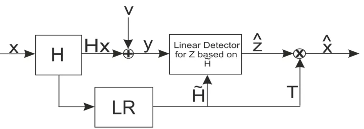
determinant of T is ±1 or ±i. Fig. 4 illustrates the block diagram of the LR-based detection scheme.

The block ‘LR’ generates the unimodular matrix Tand the new basis H˜. The model in (1) is rewritten

as

y=HTT-1x + v= ˜Hz + v, (4)

where H˜ =HTand z=T-1x. With the basis changed, the traditional detector is used to compensate for

the new channel H˜ = HT to produce the estimation of ˆz, and ˆx can be estimated through ˆx =Tˆz. In

this way, the LR algorithm is used in the linear detection equaliser.

With this new system model, linear equalisers can be applied to the channel matrix H˜ to estimate z.

When ZF and MMSE are applied to the received signal y [22–25], we obtain

ˆzZF =Q(( ˜H H_˜

H)−1H˜Hy), (5)

ˆzM M SE =Q(( ˜H H_˜

H + σ_v2THT)−1H˜Hy), (6)

Fig. 4: Block diagram of LR method in combination with linear detection equaliser for MIMO system.

ˆ

x=Tˆz. (7)

It is known that ˆx contains both the weight vector and the symbol information. Thus, wˆ is estimated as

the weight vector which has the highest correlation with the transmitted vector ˆx

b

w= arg max

ℓ

kwℓˆxk2, (8)

where ℓ ∈ {1, ...,2m_{}. The second block of data is estimated based on the estimation of the first block}

and the channel matrix, the detection ofˆs is calculated as

ˆs= (Hwˆ)−1y. (9)

As was explained, the estimation of the antenna weight vector is critical since it directly affects the

symbols estimation. Therefore, as the ABPM symbol detection is obtained in two steps, an error on the

antenna weight vector will be propagated to the APM symbol detection.

III. PERFORMANCEANALYSIS

The ABPM scheme has been described as hybrid modulation due to its combination of antenna pattern

with conventional APM schemes [18]. The ABPM transmission design changes based on the number of

Nt and beam patterns, i.e. different design for different scenario. Thus, it is not possible to derive of an

exact BER probability equation. For this reason, we derive a tight upper bound on the BER to validate

and analyse the performance of ABPM. The pairwise error probability (PEP) of an ML detector is given

Pxj →xˆj

=P hky−Hxˆj k2− ky−Hxj k2

i

≤0

=P hkHxj−xˆ_j

+vk2− kvk2i≤0

=E   Q    v u u t_2N1

0

X

j

X

ˆ_j

kHxj−xˆj

k2      . (10)

Using the union bounding technique presented in [37], the BER of ABPM is union bounded as

Pe,bit≤Exj "

X

ˆ_j

N(j,ˆj)P(xj →xˆ_j)

# ≤ L X j L X

ˆ_j,ˆ_j6=j

N(j,ˆj)

kL P(xj →xˆj),

(11)

wherekis the number of information bits carried by one ABPM symbol,jandˆj denote the indices of the

transmitted and estimated symbols,xj andxˆj respectively; Exj is the mean value of P(xj →xˆ_j),N(j,ˆj)

is the number of different bits between symbols xj and xˆj and P(xj → xˆj) is the PEP of detecting xˆj

for transmitted xj [38], which is calculated as

P(xj →xˆj) =

1−1_u 2

!_{Λ Λ−1} X

n=0 2−n

Λ−1 +n

n 1 +

1 u

!n

, (12)

where u =

s

1 + 1

ρd(j,ˆj) 2+b

, Λ = NtNr, b is the number of beams and d(j,ˆj) is the Euclidean distance

between xj and xˆj.

As expected, a larger minimum d(j,ˆj) results in better performance, similar to other conventional

modulation techniques. Substituting (12) into (11), the upper bound of the bit error probability for ABPM

can be expressed as

Pe,bit≤ L

X

j L

X

ˆ_j,ˆ_j6=j

N(j,ˆj) kL

1−1

u

2

!Λ

Λ_X−1

n=0 2−n

Λ−1 +n

n 1 +

1 u

!n

.

Note thatP EP = 0 implies no error in the detection ofxj, this is only possible ifu has the value “1”

in (12). Therefore, the accuracy of the tight upper bound depends on ifu is close to “1”. The parameter

u depends on the minimum Euclidean distanced(j,ˆj). With largerd, u is closer to “1”. Then, as d and

b are inversely related, ifb increases, d decreases and it degrades the system performance.

The upper bound indicates that larger distance between transmit vectors leads to better performance.

Therefore, it is desirable that the selected antenna beam patterns have low correlation.

IV. SIMULATION RESULTS

In this section, examples are presented in order to show the benefits achieved by ABPM. Monte Carlo

simulations are performed, and are run for at least106 channel realizations. A flat Rayleigh fading channel

with AWGN is used and perfect CSIT is assumed for simulation purposes.

Fig. 5 shows the BER performance of ABPM under different detection schemes. It compares the

optimal detector ML with high computational complexity, to an LR aided detector combined with MMSE

as a linear detector with low computational complexity, for data rates of η = 3 and 4 bits/s/Hz. When

η= 3 bits/s/Hz, two different beam patterns are used to carry QPSK, the angle difference between two

main lobes is 60◦ _{to guarantee low correlation as explained in Section II. When η = 4bits/s/Hz, it has}

four different patterns carrying QPSK, the minimum angle separation is 30◦ _{between the main beams}

γ = 0.3536(Table I), which implies that the four AoDs used are50◦_,20◦_{, −20}◦ _and−50◦_{. All schemes}

given use the same number of transmittersNt= 2 and receiversNr = 5.

It should be noted that in the case of η = 3 bits/s/Hz, the LR-MMSE has a performance very close

to that of the optimal ML detector. This is possible due to low correlation between the patterns used.

However, in the case of η = 4 bits/s/Hz, we can see a bigger difference between the two methods (2

dB at Pe,bit= 10−5). The reason for this is that the distance between transmit vectors when M = 4, is

smaller than when the system is using only 2 patterns. Another factor that impacts the BER performance,

is that the detection is made in two stages. If the estimation of the first stage (antenna beam pattern

represented by weights) is wrong, this error is carried through to the second stage which degrades the

system performance. An upper bound for each case is added when the ML detector is used. Increasing

the number of beam patterns reduces the Euclidean distance. Then, the upper bound is fairly tight with

larger Euclidean distance (two beam patterns) in comparison to that of the case of four beam patterns.

Fig. 6 depicts ABPM’s performance using both optimal and suboptimal detections in comparison with

SM [11], GSSK [12] and V-BLAST with LR aided MMSE equalisation [24] with targetedη = 3bits/s/Hz

which has QPSK modulation and two different antenna beam patterns resulting in 8 constellation points.

The first one is SM with Nt = 4 antennas and BPSK modulation. The second is SM with Nt = 2

antennas and QPSK modulation (both result inNt×M= 8constellation points). The third is GSSK with

Nt= 5, with two active transmitters. All three schemes are based on optimal ML detection. The fourth

transmission technique is V-BLAST-LR with Nt= 3, BPSK modulation and η= 3 bits/s/Hz.

ABPM’s performance with ML detection and new antenna pattern design described in this article

clearly outperforms other schemes as shown in Fig. 6, where gains of 3 dB when compared to SM 2x5

and GSSK, and more than 3.5 dB over SM 4x5 are observed at Pe,bit = 10−5. It should be noted that

the comparison between all schemes assumes identical transmission rate. To achieve the desired rate,

SM is designed with different number of transmit antennas and modulation sizes as shown in Fig. 6.

The complexity at the receiver side of these three schemes (SM, GSSK and ABPM-ML) is comparable

because they all use the ML detector. As Fig. 6 shows, ABPM-LR (dashed line) presents gains over

schemes based on SM at Pe,bit = 10−5: around 2 dB over SM 2x5 and GSSK, 2.5 dB when compared

to SM 4x5; even when the SM schemes are based on ML detection which has a higher complexity than

the linear detection used in ABPM-LR.

In comparing ABPM-LR to V-BLAST, it can be observed that the BER performance of the two is

almost the same at low values of SNR. AtPe,bit= 10−5, V-BLAST has less than 1 dB gain over

ABPM-LR. However, it should be noted that ABPM-LR uses less transmit antennas to achieve the same spectral

efficiency as V-BLAST. The advantages of using fewer transmitters are decreased costs of RF chains,

saving of physical space, reduced requirement on synchronisation and less interference between transmit

antennas. The performance gain of the ABPM- ML can be attributed to the improvement of spectral

efficiency using antenna beam patterns which permit higher transmission diversity by transmitting the

same information at each antenna. As well, it can be noticed that the upper bound is relatively tight and

support the ABPM simulation results.

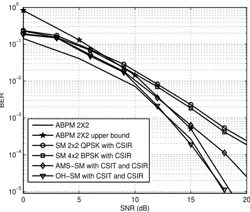
Fig. 7 shows the comparison of ABPM and SM schemes with CSIT and CSIR. An exhausted study of

SM is presented in [39,40], including an analysis of SM considering CSIT. Adaptive spatial modulation

(ASM) [41] and optimal hybrid spatial modulation (OH-SM) [42] have explored the transceiver channel

diversity through the use of CSIT to minimise the transmission rate. ASM utilises different modulation

order for different channel conditions. OH-SM is an extension of ASM, which incorporates the

trans-mission mode switching (TMS) to use different transtrans-mission modes. All the schemes have a data rate of

η= 3 bits/s/Hz. ABPM achieves gain of 1.5 dB when compared to ASM and performance similar to that

adaptive modulation and TMS require high computational complexity and the number of required bits

for feedback is large, particularly at high spatial dimension [42]. The traditional SM curves are shown in

Fig. 7 only as a reference. The upper bound is relatively tight and support the ABPM simulation results.

Fig. 8 illustrates ABPM’s performance with different number of transmit and receive antennas.

Ex-amples are presented to evaluate ABPM’s performance using the same data rate 3 bits/s/Hz with two

different antenna beam patterns and QPSK modulation. We noticed that whenNt≤Nr, ABPM has better

performance with largerNtandNr, since this scheme exploits both diversity at the transmitter and receiver

sides. However, it is also noticeable that when Nt > Nr, (such as Nt = 3, Nr = 2) the performance is

obviously degraded comparing to Nt = 2, Nr = 2 scheme. This is because each element of the vector

w is transmitted by one antenna and then multiplied with one APM symbol. This transmission process

is similar to spatial multiplexing. Then, it is expected that the constraint Nt ≤ Nr must be satisfied to

recover the signal at the receiver.

Fig. 9 illustrates the BER performance of ABPM withNt= 2,Nr= 5with two and four beam patterns

carrying 4-QAM symbols in comparison with their upper bound, with spectral efficiencies of 3 and 4

bits/s/Hz respectively. The 4-QAM with 2 beam patterns outperforms the system using 4-QAM with 4

beam patterns. The ML detector is used to demodulate the ABPM symbols. From this observation, it

is clear that increasing the number of patterns degrades the BER performance due to the fact that the

minimum distance between transmit vectors is reduced when more beam patterns are introduced. The

upper bound is presented in order to validate the results obtained by simulations as explained in section

III. It can be noticed that in the case of ABPM with 2 beams, the upper bound is tighter than ABPM

with 4 beams. The reason for this is because (13) depends on the number of beams and the Euclidean

distance. Therefore, increasing the number of beams, the value of parameter u in (13) increases, which

will impact the accuracy of the bound.

It has been demonstrated that LR in combination with linear detectors (e.g. ZF, MMSE, etc.) guarantees

a performance similar to that of the optimal detector ML but with a lower computational complexity. Fig.

10 compares the complexity between ML, LR-MMSE and MMSE detectors. It has been shown that ML

has higher computational complexity in comparison to LR-MMSE. The number of arithmetic operations

are increased when the numbers of Nt and/or Nr increase. The computational complexity increment of

LR-MMSE over MMSE is due to the calculation of the LLL algorithm to find the new basis and the

inverse ofT. As previously mentioned, ABPM has shown that using an LR-MMSE detector reduces the

0 3 6 9 12 15 10−5

10−4 10−3 10−2 10−1

SNR(dB)

BER

LR−MMSE w/4 beams ML w/4 beams upper bound ML w/4 beams

LR−MMSE w/2 beams ML w/2 beams upper bound ML w/2 beams

Fig. 5: BER performance versus SNR in comparison with ML and LR-MMSE detection for ABPM with

η= 3 and 4 bits/s/Hz.

0 3 6 9 12 15

10−5 10−4 10−3 10−2 10−1

SNR(dB)

BER

SM 4X5 SM 2X5 GSSK 5X5 n

t=2

ABPM−LR 2X5 V−BLAST−LR 3X5 ABPM−ML 2X5 ABPM 2X5 upper bound

Fig. 6: BER comparison between ABPM with optimal and suboptimal detectors, spatial modulation and

GSSK. To achieve η = 3 bits/s/Hz, ABPM uses two different transmission beam patterns and QPSK

symbols, SM uses BPSK and QPSK symbols for Nt = 4 and Nt= 2, respectively. GSSK withNt = 5

with nt = 2 active transmitters and V-BLAST transmits BPSK symbols with Nt = 3. For all systems

0 5 10 15 20 10−5

10−4 10−3 10−2 10−1 100

SNR (dB)

BER

ABPM 2X2

ABPM 2X2 upper bound SM 2x2 QPSK with CSIR SM 4x2 BPSK with CSIR AMS−SM with CSIT and CSIR OH−SM with CSIT and CSIR

Fig. 7: BER versus SNR to compare ABPM and schemes based on SM considering CSIT and CSIR.

0 5 10 15

10−5

10−4

10−3

10−2

10−1

SNR(dB)

BER

ABPM 3X2 ABPM 2X2 ABPM 2X4 ABPM 3X4 ABPM 2X6 ABPM 3X6

Fig. 8: Performance of ABPM with different MIMO scheme features (Nt and Nr), two different

0 3 6 9 12 15

10−5

10−4

10−3

10−2

10−1

SNR(dB)

BER

ABPM 2 beams

ABPM 2 beams upper bound ABPM 4 beams

ABPM 4 beams upper bound

Fig. 9: BER versus SNR for 4-QAM modulation scheme with 2 and 4 beam patterns and their respective

upper bounds.

2 4 6 8 10 12 14 16

0 0.2 0.4 0.6 0.8 1 1.2 1.4 1.6 1.8

2x 10

5

Total number of antennas N

t=Nr

Number of Arithmetic Operations

ML LR−MMSE MMSE

V. CONCLUSION

A deeper study about the work done in [18] regarding transmission and detection design for the antenna

beam pattern modulation (ABPM) has been presented. The antenna patterns are selected to minimise their

correlation. A new LR-aided algorithm combined with MMSE is proposed as suboptimal detection to

achieve performance which is similar to that of the optimal ML detector but with lower computational

complexity. The BER results show that the ABPM-LR outperforms SM/ML and GSSK/ML by around 3

dB. An analytic upper bound has been derived to validate the simulation results. The antenna beam pattern

modulation performance has indicated that it is a promising candidate for low complexity transmission

techniques in future generations of communications systems such as in massive MIMO.

APPENDIX

Upper Bound Derivation

In this appendix we demonstrate the derivation of the upper bound for MIMO block fading channel. For

coding systems, the PEP forms the basic structure for the union bound calculation of the error probability

and is utilised as the main criteria for code design. The PEP between two arbitrary code-words c and e

overN time slots in the Rayleigh fading channel [38] is expressed as

P(c→e) = 1−

Z

Rm

p(c|x)dx

= aEw

" Q v_u u t Nt X

j=1 Nr

X

v=1

|wv j |2

!#

,

(A.14)

where Rm is the decision regions, p(c|x) is the joint probability density function (PDF), a = _4NE_ts_No,

Es is the symbol energy, No is Gaussian noise variance and |wv_j |is Rayleigh distributed.

Denote w=w1₁ andzv_j = wv1

w, (j,v)6=(1,1). Their joint PDF,f(w,z v

j· · ·zNNrt)can be obtained from their cumulative density function F(w,zv_j· · ·zNr

Nt) and expressed as

f(w,zv_j· · ·zNr Nt) = w

2NtNr−1_·

Nt Y j=1 Nr Y v=1 (j,v)6=(1,1)

zv_je−

w2

2

1+PNtj=1

PNr

v=1 (j,v)6=(1,1)(z v j)2

One of the properties of the complementary Gaussian cumulative distribution function (Q-function) is

the integral property [43], which is expressed

Z ∞

0

x2n−1e−x

2 2 Q(x

σ)dx

= (n−1)!

2 (1−(σ

2_{+ 1)}−1 2)n

×

n−1

X

k=0 2−k

n−1 +k k

(1 + (σ2+ 1)−12)k.

(A.16)

Utilising (A.15) and (A.16), the PEP can be expressed as

P(c→e) = 1− 1

u

2

!_{Λ Λ−1} X

k=0 2−k

Λ−1 +k

k 1 +

1 u

!k

, (A.17)

where u=

r

1 +1

a,Λ =NtNr.

REFERENCES

[1] S. Alamouti, “A simple transmit diversity technique for wireless communications,”IEEE J. Sel. Areas Commun., vol. 16,

no. 8, pp. 1451–1458, 1998.

[2] V. Tarokh, N. Seshadri, and A. Calderbank, “Space-time codes for high data rate wireless communication: Performance

criterion and code construction,”IEEE Trans. Inf. Theory, vol. 44, no. 2, pp. 1185–1191, 1998.

[3] P. Wolniansky, G. Foschini, G. Golden, and R. Valenzuela, “V-BLAST: An architecture for realizing very high data rates

over the rich-scattering wireless channel,” inURSI Int. Symp. Signals, Syst. and Electron. (ISSSE) 1998. IEEE, 1998, pp.

295–300.

[4] L. Zheng and D. Tse, “Diversity and multiplexing: A fundamental tradeoff in multiple-antenna channels,”IEEE Tran. Inf.

Theory, vol. 49, no. 5, pp. 1073–1096, 2003.

[5] V. Tarokh, A. Naguib, N. Seshadri, and A. Calderbank, “Combined array processing and space-time coding,”IEEE Trans.

Inf. Theory, vol. 45, no. 4, pp. 1121–1128, 1999.

[6] M. Chiani, M. Z. Win, and A. Zanella, “On the capacity of spatially correlated MIMO Rayleigh-fading channels,”IEEE

Trans. Inf. Theory, vol. 49, no. 10, pp. 2363–2371, 2003.

[7] M. O. Damen, A. Abdi, and M. Kaveh, “On the effect of correlated fading on several space-time coding and detection

schemes,” in54th Veh. Technol. Conf. (VTC) 2001 Fall, vol. 1. IEEE, 2001, pp. 13–16.

[8] R. Mesleh, H. Haas, C. Ahn, and S. Yun, “Spatial modulation: A new low complexity spectral efficiency enhancing

technique,” in1st Int. Conf. Commun. and Network. (ChinaCom) 2006, 2006, pp. 1–5.

[9] R. Mesleh, H. Haas, S. Sinanovic, C. Ahn, and S. Yun, “Spatial modulation,”IEEE Trans. Veh. Technol., vol. 57, no. 4,

pp. 2228–2241, 2008.

[10] A. ElKalagy and E. AlSusa, “A novel two-antenna spatial modulation technique with simultaneous transmission,” in17th

[11] J. Jeganathan, A. Ghrayeb, and L. Szczecinski, “Spatial modulation: optimal detection and performance analysis,”IEEE

Commun. Lett., vol. 12, no. 8, pp. 545–547, 2008.

[12] ——, “Generalized space shift keying modulation for MIMO channels,” inIEEE 19th Int. Symp. Pers., Ind. and Mobile

Radio Commun. (PIMRC) 2008, 2008, pp. 1–5.

[13] A. Younis, N. Serafimovski, R. Mesleh, and H. Haas, “Generalised spatial modulation,” in44th Conf. Signals, Syst. and

Comput. (ASILOMAR) 2010. IEEE, pp. 1498–1502.

[14] R. Ramirez-Gutierrez, L. Zhang, J. Elmirghani, and R. Fa, “Generalized Phase Spatial Shift Keying Modulation for MIMO

Channels,” in73rd Veh. Technol. Conf. (VTC Spring) 2011, may 2011, pp. 1 –5.

[15] A. Kalis, A. G. Kanatas, and C. B. Papadias, “A novel approach to MIMO transmission using a single RF front end,”

IEEE J. Sel. Areas Commun., vol. 26, no. 6, pp. 972–980, 2008.

[16] O. N. Alrabadi, C. B. Papadias, A. Kalis, and R. Prasad, “A universal encoding scheme for MIMO transmission using a

single active element for PSK modulation schemes,”IEEE Trans. Wireless Commun., vol. 8, no. 10, pp. 5133–5142, 2009.

[17] K. Antonis, C. Papadias, and A. Kanatas, “An ESPAR Antenna for Beamspace-MIMO Systems Using PSK Modulation

Schemes,” inIEEE Int. Conf. Commun. (ICC) 2007, june 2007, pp. 5348 –5353.

[18] R. Ramirez-Gutierrez, L. Zhang, J. Elmirghani, and A. Almutairi, “Antenna Beam Pattern Modulation for MIMO Channels,”

in8th Int. Wireless Commun. and Mobile Comput. Conf. (IWCMC) 2012. IEEE, 2012, pp. 591–595.

[19] Y. Jiang, M. Varanasi, and J. Li, “Performance analysis of ZF and MMSE equalizers for MIMO systems: an in-depth study

of the high SNR regime,” vol. 57, no. 4. IEEE, 2011, pp. 2008–2026.

[20] J. Cassels,An introduction to the geometry of numbers. Springer Verlag, 1997.

[21] J. Niu and I. Lu, “A new lattice-reduction-based receiver for MIMO systems,” in41st Annu. Conf. Inf. Sci. and Syst. (CISS)

2007. IEEE, 2007, pp. 499–504.

[22] D. Wubben, R. Bohnke, V. Kuhn, and K. Kammeyer, “Near-maximum-likelihood detection of MIMO systems using

MMSE-based lattice reduction,” inIEEE Int. Conf. Commun., vol. 2. IEEE, 2004, pp. 798–802.

[23] H. Yao and G. Wornell, “Lattice-reduction-aided detectors for MIMO communication systems,” inIEEE Global

Telecom-mun. Conf. (GLOBECOM) 2002, vol. 1. IEEE, 2002, pp. 424–428.

[24] X. Ma and W. Zhang, “Performance analysis for MIMO systems with lattice-reduction aided linear equalization,”IEEE

Trans. Commun., vol. 56, no. 2, pp. 309–318, 2008.

[25] Y. Gan, C. Ling, and W. Mow, “Complex lattice reduction algorithm for low-complexity full-diversity MIMO detection,”

IEEE Trans. Signal Process., vol. 57, no. 7, pp. 2701–2710, 2009.

[26] A. Lenstra, H. Lenstra, and L. Lov´asz, “Factoring polynomials with rational coefficients,” Mathematische Annalen, vol.

261, no. 4, pp. 515–534, 1982.

[27] J. Hoydis, S. Ten Brink, and M. Debbah, “Massive MIMO: How many antennas do we need?” in49th Annu. Allerton

Conf. Commun., Control and Comput. IEEE, 2011, pp. 545–550.

[28] J. Andrews, A. Ghosh, and R. Muhamed,Fundamentals of WiMAX: understanding broadband wireless networking. Prentice

Hall PTR, 2007.

[29] M. Leng and Y.-C. Wu, “Low-complexity maximum-likelihood estimator for clock synchronization of wireless sensor

nodes under exponential delays,”IEEE Trans. Signal Process., vol. 59, no. 10, pp. 4860–4870, 2011.

[30] C. Windpassinger and R. F. Fischer, “Low-complexity near-maximum-likelihood detection and precoding for MIMO

[31] D. Wubben, R. Bohnke, V. Kuhn, and K.-D. Kammeyer, “MMSE extension of V-BLAST based on sorted QR

decomposition,” in58th Veh. Technol. Conf. (VTC) 2003-Fall, vol. 1. IEEE, 2003, pp. 508–512.

[32] F. T. Luk, S. Qiao, and W. Zhang, “A lattice basis reduction algorithm,”Institute for Computational Mathematics Technical

Report 10, vol. 4, 2010.

[33] E. Agrell, T. Eriksson, A. Vardy, and K. Zeger, “Closest point search in lattices,”IEEE Trans. Inf. Theory, vol. 48, no. 8,

pp. 2201–2214, 2002.

[34] M. Taherzadeh, A. Mobasher, and A. Khandani, “Lattice-basis reduction achieves the precoding diversity in MIMO

broadcast systems,” in39th Conf. Inf. Sci. and Syst. (CISS) 2005, 2005.

[35] P. Q. Nguyen and B. Valle, The LLL algorithm: survey and applications. Springer Publishing Company, Incorporated,

2009.

[36] Q. Zhou and X. Ma, “Element-Based Lattice Reduction Algorithms for Large MIMO Detection,” IEEE J. Sel. Areas

Commun., vol. 31, no. 2, pp. 274–286, 2013.

[37] J. Proakis and M. Salehi,Digital communications. McGraw-hill New York, 2001, pp. 261–262.

[38] Z. Lin, E. Erkip, and A. Stefanov, “The exact pairwise error probability for MIMO block fading channel,” in Proc. Int.

Symp. Inf. Theory Appl. Citeseer, 2004, pp. 728–732.

[39] M. Di Renzo, H. Haas, A. Ghrayeb, S. Sugiura, and L. Hanzo, “Spatial modulation for generalized MIMO: challenges,

opportunities, and implementation,”IEEE Proc., vol. 102, no. 1, pp. 56–103, 2014.

[40] M. Di Renzo, H. Haas, A. Ghrayebet al., “Spatial modulation for MIMO wireless systems,” inIEEE Wireless Commun.

Network Conf. WCNC 2013, 2013.

[41] P. Yang, Y. Xiao, Y. Yu, and S. Li, “Adaptive spatial modulation for wireless MIMO transmission systems,”IEEE Commun.

Lett., vol. 15, no. 6, pp. 602–604, 2011.

[42] P. Yang, Y. Xiao, L. Li, Q. Tang, Y. Yu, and S. Li, “Link adaptation for spatial modulation with limited feedback,”IEEE

Trans. Veh. Technol., vol. 61, no. 8, pp. 3808–3813, 2012.