Rochester Institute of Technology
RIT Scholar Works
Theses Thesis/Dissertation Collections
5-19-2017
Identification of Differential Expression of p53
associated RNAs at 3 Different Treatment
Timepoints, and Association with ChIP-seq
Identified p53 Genes.
Julia Freewoman
Follow this and additional works at:http://scholarworks.rit.edu/theses
This Thesis is brought to you for free and open access by the Thesis/Dissertation Collections at RIT Scholar Works. It has been accepted for inclusion in Theses by an authorized administrator of RIT Scholar Works. For more information, please [email protected].
Recommended Citation
R.I.T.
Identification of Differential Expression
of p53 associated RNAs at 3 Different
Treatment Timepoints, and Association with
ChIP-seq Identified p53 Genes.
by
Julia Freewoman
A Thesis Submitted in Partial Fulfillment of the Requirements
for the Degree of Master of Science in Bioinformatics.
School of Thomas H. Gosnell School of Life Sciences
Bioinformatics Program
College of Science
ii
Thesis Committee Members:
Feng Cui, Ph.D., thesis advisor
Andre Hudson, Ph.D.
iii
Table of Contents
Abstract ... 1
I. Introduction ... 1
II. Materials and Methods ... 6
A. Cell Culture ... 6
B. RNA Extraction. ... 7
C. Illumina Sequencing ... 7
D. FASTQ Filtering and Quality Assessment... 8
F. Alignment and Differential Analysis ... 8
G. CummeRbund and Timepoint Analysis ... 11
H. GO Enrichment Analysis ... 15
I. Image Production ... 16
J. ChIP-qPCR ... 18
IV. Results and Discussion ... 19
A. Quality Control ... 19
B. Timepoint Differential Analysis... 24
C. Non-protein Coding RNA ... 33
D. Expression and Imaging. ... 35
E. GO Enrichment ... 45
F. ChIP-qPCR. ... 48
V. Conclusions ... 50
Acknowledgements ... 56
References ... 57
Table of Figures Figure 1: Overall Flow of Design of the Study... 6
Figure 2: Cufflinks Flow Through, from Cufflinks Website: ... 10
Figure 3: Quality Score Comparison: ... 20
Figure 4: Number of Reads: ... 21
Figure 5: Differential Analysis Quality Metrics: ... 23
Figure 6: Scatterplotmatrix for All Treatments: ... 24
Figure 7: Heatmaps: ... 27
Figure 8: Venn Diagrams for RNA-seq and ChIP Genes: ... 30
Figure 9: Venn Diagrams for RNA-seq and 5kb ChIP Genes: ... 31
Figure 10: Protein Coding and All Genes, Regulation by Timepoint: ... 32
Figure 11: Non-coding RNA Genes Regulation by Timepoint: ... 34
iv
Figure 13: Expression of CDKN1A and TP53I3: ... 40
Figure 14: Expression of BBC3 and BAX:... 41
Figure 15: Expression of SMAD3 and MDM2: ... 42
Figure 16: Expression of HAUS6 and SAC3D1: ... 43
Figure 17: Expression GAPDH ... 44
Figure 18: Expression of Non-coding RNA Examples: ... 45
Figure 19: GO Biological Term Fold Enrichment Top Significant Terms: ... 47
Figure 20: GO Terms Full Descriptions: ... 48
Figure 21: ChIP qPCR of p53 target genes:... 50
v
Table 1: Abbreviations
Abbreviation Full name and description
p53
Tumor protein p53. Major protein responsible for the regulation of the cell cycle and inducement of cell cycle arrest or cell death ( apoptosis )
G1
Gap phase prior to S phase and DNA replication. One of the the two phases p53 where induces cell arrest or apoptosis
G2
Gap phase prior to M phase involving nuclear division and cytoplasmic division. One of the two phases p53 where induces either cell arrest or apoptosis .
CDKN1A
Cyclin Dependent Kinase Inhibitor 1A, also known as p21. Regulates the cell cycle progression past the G1 phase, and is tightly controlled by p53.
BBC3
BCL2 Binding Component 3, also known as PUMA. Gene that has been strongly associated with the p53 signaling pathway.
BAX
BCL2 Associated X, Apoptosis Regulator. Responsible for p53 mediated apoptosis and strongly associated with p53 signaling.
5-FU 5-fluorouracil. Drug used to induce p53 pathway.
FPKM
Expected fragments per kilobase of transcript per million fragments sequenced, used as a scalar for expression data
lincRNA
Long intergenomic non-coding RNAs. RNAs of 200bp or greater in length that do not encode for proteins and do not overlap with any protein coding genes
miRNA microRNA. RNAs of approximately 22 bp in length.
ERV1
ERV1/LTR. A subclass of endogenous retroviruses (ERVs or LTR retrotransposons), which are a type of retrotransposons with an LTR (long terminal repeat)
ChIP-seq Chromatin Immunoprecipitation sequencing
HCT116 Human cell line derived from colon cancer
High Throughput
Sequencing Next Generation Sequencing
FDR False Discovery Rate. Modified p value denoted with a q instead of a p.
HG19 Version of the human genome produced in 2009.
TP53I3 Tumor Protein P53 Inducible Protein 3. Gene known to be induced by p53.
SMAD3 SMAD Family Member 3. Signaled by TGF-?, and interacts with p53 pathway.
MDM2
MDM2 Proto-Oncogene. Major regulator of p53, responsible for degradation of p53 protein, and regulated by p53
HAUS6
HAUS Augmin Like Complex Subunit 6. Associated with chromosome congression and segregation
SAC3D1
SAC3 Domain Containing 1. Paralog for MCM3AP, which is essential for DNA replication.
read The sequence of one cluster sequenced during High Throughput Sequencing.
1
Abstract
Called “the guardian of the genome,” p53 is one of the most studied proteins associated
with cancer. After activation, p53 induces its target genes with different kinetics, i.e., early
induction or delayed induction. However, this difference in kinetics of gene induction has not
been examined genome-wide. This study uses RNA-seq time course data (0-hour, 6-hour,
12-hour and 24-12-hour) via drug induction with 5-fluorouracil (5-FU), and compares that data to
previously published ChIP-seq data. We found that, while there is an induction of a number of
genes at 6 hours, there appears to be a delayed phase of induction occurring at 24 hours,
including some of the genes that have been upregulated previously, such as CDKN1A and
BBC3. Combining published ChIP-seq data, we are able to narrow our dataset to a select group
of genes of particular interest, which are associated with known p53 functions such as apoptosis
and cell cycle arrest. We propose that the early phase of induction is due to existing p53 proteins
in cells, while the delayed phase of induction is probably due to accumulation of the p53 protein
and lack of degradation of p53 protein, which is likely related to its interactions with MDMX
and MDM2.
I. Introduction
Originally identified in 1979 [1], p53 has come to be referred to as the “guardian of the
genome,” since it is responsible for regulation of the cell cycle [2]. If induced due to cell stress,
p53 will induce either cell cycle arrest at the G1 or G2 stage, or apoptosis (cell death) [2].
2 p53’s importance in cancer and the regulation of the cell cycle, understanding which genes p53
regulates, and how it interacts with them, is an active area of research.
Given its status as ‘“guardian of the genome,”’ p53 is, in all likelihood, a transcription
factor, and it directly and indirectly is responsible for the inducement of other proteins important
for the regulation of cell cycle arrest/cell death [4]. Therefore, in the study of p53 and its
regulation of the cell cycle, including discovering how and when p53 binds to and regulates
particular genes, is important, and an ongoing area of investigation—in particular, discovering
where p53 binds to the genome during stress, since p53 transcription is increased during cell
stress, and its increased activation can lead to cell death [4] [5] [2]. Among the discovered genes
associated with the p53 pathway are CDKN1A(p21), BBC3 (PUMA) and BAX, which are now
often used as indicators of p53 activity [6] [7]. Inducing a stress response in cultured cells is
achieved through the use of drug 5-fluorouracil (5-FU), or through introduction of other
stressors, such as UV light [5].
Along with genes, other non-protein coding RNAs can have possibly important
regulatory or other interactions with the p53 pathway. Among these RNAs are lincRNAs (long
intergenomic non-coding RNAs), miRNA (microRNAs) and ERV1/LTR. LincRNAs are part of
a larger group, although they are the most important of the group of lncRNAs (long non-coding
RNAs) which are defined as being larger than 200 bp, although they can be much larger—up to
tens of Kilobases in length [8]. LincRNAs are a subset of lncRNAs, but they may not overlap
with any protein coding regions [9]. Of particular interest for this study is the fact that lincRNAs
have been linked to the p53 regulatory network [8]. MicroRNAs are defined as being around 22
bp (nt) in final length, and have been found to play important roles in regulation and degradation
3 subclass of endogenous retroviruses (ERVs or LTR retrotransposons), which are a type of
retrotransposons with an LTR (long terminal repeat) [12]. ERV1s in cancer have been shown to
upregulate lncRNAs (which lincRNAs are a subclass of) in cancer, and are often upregulated in a
cancers, and since 50% of cancers have a mutated p53 gene, investigation of ERV1 is of interest
[13].
Two of the best ways to determine genes associated with upregulation of p53 are
RNA-seq and ChIP. RNA-RNA-seq, as the name implies, is the RNA-sequencing of resulting RNA from cells or
tissue under stressful or non-stressful conditions [14]. After RNA extraction, the extracted RNA
is then sequenced using High Throughput Sequencing techniques such as Illumina [14]. To
determine the genes that are activated by p53, either directly or indirectly, stressed conditions
must be compared to non-stressed conditions to determine the decrease or increase of gene
expression.
Alternatively, Chromatin Immunoprecipitation (ChIP) can be used to determine which
genes p53 is a transcription factor for. Until recently, the most sensitive version has been
ChIP-seq [15]. ChIP-ChIP-seq is an adaptation of the original ChIP. The reason ChIP-ChIP-seq is one of the most
sensitive ways to determine where a particular protein interacts with the chromatin is because
ChIP is designed to isolate sections of DNA. It does this first by crosslinking any proteins
associated with parts of the genome; the proteins are essentially stuck in place via a crosslinking
agent, usually formaldehyde [16]. The cells are then lysed, and the DNA fragments, with
crosslinked proteins, are then sheared to an appropriate size range (100-500 bp in the case
ChIP-seq), and the protein of interest is selected through the use of an antibody-inoculated bead [16].
The DNA is then removed from the beads and purified [16]. This enrichment of DNA fragments
4 allows ChIP to determine the sites p53 associates with, especially during stress events. The
difference between ChIP and ChIP-seq is the use of High Throughput sequencing, which makes
it possible for the entire genome to be sequenced, thus allowing for more sensitivity and better
determination of regions where p53 is associated [15].
One cell line often used in this process is HTC116, which was first derived from colon
cancer in 1981 [17], and which originally was homozygotic wildtype p53 (HTC116 +/+) [18].
This study will use the HTC116 +/+ cell line to investigate RNA-seq at 0, 6, 12, and 24 hours of
5-FU in comparison with previously identified ChIP-seq genes [7] [19] [20]. This will allow the
determination of which genes occur in both the RNA-seq and ChIP-seq datasets but also how the
identified genes are up or downregulated at different drug timepoints.
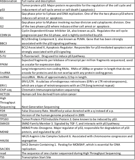
This study used RNA-seq data, which was aligned using the Cufflinks pipeline extracted
from HTC116 p53 +/+ cells treated at 6, 12, and 24 hours with 5-FU, along with a non-treatment
control, as can be seen in Figure 1. As can be seen in Figure 1, the differentially expressed genes
at each different timepoint were determined through the use of CummeRbund. Once the
differentially expressed genes had been determined for each timepoint, including the control, the
RNA-seq dataset was then subseted for genes that also had been reported in previous ChIP-seq
studies. As can be seen in Figure 1, once the ChIP-seq subsets were created, each set was
analyzed for differential expression of control, different RNA types, and finally, a GO analysis
was run for subset. Finally, as a verification, the initial steps of a ChIP-seq experiment were
performed, and with the % input for CDKN1A and BBC3. Overall, this study showed that there
is an initial induction at 6 hours, for most genes, that is followed by a further induction at 24
hours. This was observed for all RNA-seq genes as well as those also found in the ChIP-seq data,
5 Additionally, through the comparison with ChIP-seq data, it appears that the dataset can be
narrowed to a select group of genes of particular interest, which are actively associated with
apoptosis and p53. This was seen through a comparison of GO Enrichment results between
subsets of RNA-seq and intersected RNA-seq and ChIP-seq data. The results of the RNA-seq
appear to be validated by the initial results of a ChIP-seq experiment using the same timepoints
via % input for CDKN1A and BBC3, and showed the same pattern of association of p53 as can
be seen with the expression of those same genes. The model proposed is that secondary
upregulation occurring at 24 hours is due to accumulation of the p53 protein and the lack of
degradation of new p53 protein, possibly due to MDMX associating with MDM2; while the
increase at 6 hours is due to the already-existing p53 protein in the cell.
6
Figure 1: Overall Flow of Design of the Study.
II. Materials and Methods
A. Cell Culture
All HTC116 p53 +/+ (John Hopkins University GRCF Biorepository & Cell Center,
Catalog Number: 8) were grown in recommended McCoy’s 5a modified media (Life
Technologies, Catalog Number: 16600-082) with 10% FBS. In addition, a 1X antibiotic mix was
added to reduce the chances of contamination (Life Technologies, catalog number: 15240-062) Extract RNA
(control, 6, 12, and 24 hours)
Send for Illumina sequencing Filter and cutadapt returned (cleaned) Sequences Quality (FastQC) filtered and cutadapted sequences
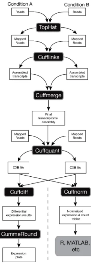
Align to HG19 genome using TopHat Differential Analysis (figure 2) Quality assessment of differential analysis using Cufflinks Extract significant differentially expressed genes using cummeRbund
Sort and report significant
genes at different timepoints Determine significant differntially expressed genes for control Determine intersections for each timepoint for RNA of interest
7 was added to the McCoy’s 5a modified media with 10% FBS. Cells where grown in the media
described at 37º C with 5% CO2. For each experimental replicate, the cells were grown in a 35
mm plates until 70-80% confluent, at which point, either 6, 12 or 24 hours prior to RNA
extraction, the media was changed, and 2 ml of fresh media, along with 375 µM 5-FU in DMSO,
were added to the 70-80% confluent cells. In addition, there was a non-treatment control—which
consisted of simply McCoy’s 5a modified media with 5% FBS and 1X antibiotic mix. Then
RNA extraction occurred when the cells reached confluence, with media being changed at least 6
hours prior to RNA extraction.
B. RNA Extraction.
For each treatment, a total of 2 replicates per treatment, the RNA was extracted using the
QUIAGEN RNeasy Mini Kit (QIAGEN, catalog number: 74104) and the QIAshredder
(QIAGEN, catalog number: 79654) during the RNeasy Kit’s lyse and homogenization stage. The
directions for each kit were followed, and the concentration after extraction was determined
using a nanodrop. The samples were kept in the -21 ͦ C until they were sent to University of
Rochester Genomics Research Center (URGRC) for sequencing, and the remaining RNA was
stored at -80 ͦ C for possible further use.
C. Illumina Sequencing
Following RNA extraction, each sample was sent to University of Rochester Genomics
Research Center (URGRC) for Illumina sequencing with at least 10 µl of sample, which had
more than the minimum required amount of 15 ng of RNA required by URGRC. At URGRC,
once the samples had been accessed for quality and sequenced, the sequenced reads were cleaned
8
D. FASTQ Filtering and Quality Assessment.
Once the High Throughput Sequenced files were received from URGRC, the FASTQ
files in the “cleaned” folder—those that had been cleaned (adapters removed and quality filtered
and reads with size lower than 25 bp filtered out)—were filtered for a quality score at least 28
over 90% of the read using the Hannon lab’s FASTX-toolkit (version 0.0.13) fastq_quality_filter
tool, which can be found at: http://hannonlab.cshl.edu/fastx_toolkit,. Following the FASTX
filter, cutadapt (version 1.10) [22] was used to filter out all reads smaller than 50bp, which was
the preference of our lab, and larger than 30-75 bp, as suggested by the Encode Project [23].
Before continuing on to alignment, the quality of each replicate was assessed using FastQC
(0.11.4) (found at: http://www.bioinformatics.babraham.ac.uk/projects/fastqc/) to ensure that
large amounts of data had not been lost due to filtering and there were no other quality issues that
might affect the overall analysis.
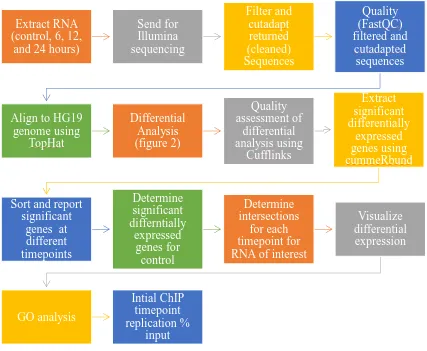
F. Alignment and Differential Analysis
Prior to alignment with the HG19 genome, of which the GTF file was downloaded from
iGenomes, Bowtie 2 indexes were constructed using a combined HG19 genome fa file and the
iGenomes HG19 GTF file, using Bowtie’s bowtie2-build (Bowtie2 version 2.2.9). Following the
construction of the Bowtie 2 indexes, TopHat (version 2.1.1) Transcriptome files were produced
to reduce the overall time required by TopHat for each individual alignment [24]. Once the
Transcriptome files were produced, and each was cleaned and filtered, the FASTQ sequencing
file was aligned to the HG19 genome using TopHat, with BAM files not being converted to
9 The produced BAM files were later sorted using SAM-tools (version 1.3.1), for visualization
using the IGV browser [26].
Once the BAM (accepted_hits.bam) files had been produced for each sample (replicate
and treatment), Cufflinks (version 2.2.1) [27] [28] was used for differential analysis. The
pipeline as suggested by the developers of Cufflinks can be seen in Figure 2. In brief, Cufflinks
was run for each sample and produced an individual GTF file; following that, Cufflinks’
Cuffmerge merged the GTF files into one GTF; Cuffquant was then run for each BAM file and
the merged GTF file, which then produced a CFX file; and finally, Cuffdiff was run using each
CFX file, with the replicates for each treatment combined under one label, as well as the required
merged GTF file was also added for Cuffdiff [28]. The -g (reference annotation) for Cufflinks
and Cuffmerge was used, and the reference genome (HG19) was formatted as suggested by
Cufflinks and downloaded from iGenomes [29]. Additionally, -b (fragmentation biases
correction) was used with the provided HG19 genome file, as well as -u (multi-read correction),
which improved the accuracy weights reads located in different parts of the genome. These
options were available for Cufflinks, Cuffquant, and Cuffdiff [30]. When available, the labeling
and renaming options were used; otherwise, all options were left at defaults. Once finished, the
10
Figure 2: Cufflinks Flow Through, from Cufflinks Website:
Shows the flow through for both versions of Cufflinks previous to 2.2.0 and the flow through for versions 2.2.0 and greater than 2.2.0, We used the 2.2.0 and greater flow through. Image is modified from the Cufflinks manual website at
http://cole-trapnell-lab.github.io/cufflinks/manual/
11
G. CummeRbund and Timepoint Analysis
Upon finishing the differential analysis, the first step was to check quality using
CummeRbund [31]. This included verifications of a normal curve using cDensity function,
normal curve occurring between the same treatments, a good linear regression between two
different treatments using csScatterMatrix function, and, finally, replicates grouping using the
csDendro function for the gene level.
Once the quality control was verified for all the samples, it became necessary to match
the identified ChIP genes with the significant RNA-seq genes generated for each timepoint (0hr,
6hr, 12hr, and 24hr). To this end, the matrix with the tracking id (XLOCs).
3associated with the gene name, which is the universal gene code, or NA if the location
did not exist in the GTF file, was created. Additionally, for each treatment comparison (i.e. 0hr
vs 6hr), all the significant tracking IDs were selected using the getSig command with
alpha=0.05, and level=gene. The significant IDs were then used in the getGenes command to
produce a cuffset, which was then used with the diffData command to produce a table of all the
differentially expressed data in the cuffset. That table was then subset for only the significant
genes (those with an FDR q=0.05), only showing a comparison between the treatment
comparison, and finally subset for both up and down regulation compared to the treatment with
fewer hours. Additionally, this step was skipped for the full dataset. Finally, both matrixes were
merged and a CVS with the data was produced Treatment pairs were used instead of one file
of all significant genes because the merge did not work of if there were replicate tracking IDs in
the differentially expressed data table. This data is the RNA-seq data discussed in the rest of this
12 Previously the ChIP-seq data from Botcheva and McCorkle, Sanchez et al., and We et al.
[7] [19] [20] had been processed and the unique fragments for all the datasets reported a long
with the closet TSS site and the associated gene name [32]. This data was used for the ChIP-seq
data that would be compared to the RNA-seq significant data just produced. Prior to the
comparison between the ChIP dataset and the RNA-seq dataset the ChIP data needed to
restructure to HG19. Due to identified lncRNA locations found in the UCSC Genome Browsers
[33] only be available starting with HG19, and the ChIP dataset being in HG18 the ChIP dataset
needed to be converted to HG19 via the Batch Coordinate Conversion tool (liftOver) found at the
UCSC Genome Browser [33]. Since, the Batch Coordinate Conversion tool only worked for
BED format that the ChIP data had both the ChIP identified site (labeled gene in the file) and the
nearest TSS site (TSS in the file) two BED files were produced with gene names plus a digit
(BBC_1 for example being the gene BBC and the first entry) so that the ChIP data could be
matched together and reformed after the conversion. Additionally, to deal with any issues where
a ChIP of mismatched names the RNA-seq location data was compared to the ChIP data if the
TSS site was more than 5kb from the TSS and the RNA-seq location was less than 5kb from the
ChIP or intersecting and the identified RNA-seq gene was not “NA” (indicting it did not occur in
the GTF file) then the RNA-seq name replaced the TSS indicated name and the RNA-seq
location information was put in TSS location information. Additionally, two ChIP files were
produced one with TSS sites or RNA-seq sites less than 5kb or intersecting and one with all of
the replaced sites and ChIP sites.
Once the ChIP files had been produced they were compared to the RNA-seq
differentially expressed data. First, before the comparison occurred the “NA” genes, RNA-seq
13 compared (all or 5kb) and if the RNA-seq location was within 5kb of the ChIP site or the TSS
site or intersected either one then “NA” was replaced with the ChIP gene name. Once, all of the
ChIP data was prepared the RNA-seq the RNA-seq data was sorted into sorted into groups
(control, 6 hour, 12 hour and 24 hour). The ChIP dataset was then compared to the RNA-seq
dataset and if the ChIP-seq gene matched the gene name of the seq gene name or an
RNA-seq gene was closer to the ChIP-RNA-seq site than the identified TSS site then the ChIP-RNA-seq gene was
added to the ChIP-seq dataset if the ChIP site was within 5kb of the TSS site it was added to the
5kb ChIP dataset. The hour groups from RNA-seq data were used in the ChIP-seq groups.
Following the sorting time sets were search for a list of genes of interest (CDKN1A, BBC3,
BAX, TP53I3, SMAD3, MDM2, HAUS6, and SAC3D1) and the time comparisons in which
each gene was found to be significant were printed out into a file. Additionally, the differentially
expressed XLOCs were written into 3 different files, one for all differential expression, those that
intersected with any ChIP gene, and those that intersected with ChIP genes 5kb or less.
Additionally, the XLOC IDs for the genes of interest were also written to a separate file. These
files were used to create subsets for heatmaps and other images later on. In addition, the amount
of differentially expressed genes for each treatment vs the control was of particular interest and
the number of genes that were differentially expressed vs control for each treatment time were
determined along with the number of genes found to be differentially expressed for two
treatment points and all of them vs the non-treatment control. This was done for both up and
downregulated differentially expressed sets along and for both ChIP datasets.
Once the initial timepoint analysis was done and assured to be working correctly,
differential expression at different timepoints, and for different types of RNA expression, were
14 by CummeRbund covers. To this end, a combination of gene_id (XLOC) and tss_id
(transcript_id) was used. The locations were determined from the merged GTF file produced by
Cuffmerge. Unlike the original GTF, this GTF file included the locations of transcripts that were
not included in the original GTF file, which would otherwise have ended with gene name labels
of “NA”. The start of any particular tss_id XLOC combination was the smallest location listed
for the start of that particular tss_id, and the end was the furthest location listed for that particular
tss_id. The location, along with the combined name (i.e. XLOC_015380-TSS24591), was printed
in the BED file to be used to create a custom track in the UCSC Genome Browser [35].
Using the UCSC table browser [36], one can download or compare tracks [34] to ensure
that the intersections between the RNA-seq data and these tracks was for only the genetic
elements of interest (only protein coding genes, for example). Each UCSC browser track was
downloaded, and material not of interest was edited out. The tracks used were lincRNA
RNA-seq Reads using the colon table, lincRNA Transcripts [9] [27], sno/miRNA [10] [11] [37], and
RefSeq Genes [38] [39]. Additionally, using LTR/ERV1 sites identified from previously
identified LTR/ERV1 sites [32], a user-defined track was created. The RefSeq Genes track was
sorted so it only contained coding genes (noted as mRNA) and then reloaded back into the
UCSC Genome Browser. Here, any intersections between the RNA-seq locations and RefSeq
locations were found using the default settings in the UCSC Genome Browser. Two different
BED files were produced, one that had the names of the protein coding genes, and the other that
contained the names for the RNA-seq IDs. Both files had the locations of those named elements.
Both lincRNA RNA-seq reads and lincRNA transcript tracks have transcripts of unknown coding
potential in them (identified as names starting with tcons_l2). These were filtered out for both
15 back into the UCSC Genome Browser and intersected with the RNA-seq location file for any
overlapping transcripts. Again, two files were produced. However, those files were intersected
with the RefSeq mRNA track, and only those that didn’t intersect printed out into the two files.
The sno/miRNA track was sorted so only the locations for type miRNA remained. Again, this
track was then loaded back into the browser and intersected with the RNA-seq track, and the
names and two BED files were produced. Finally, a BED file with LRT/ERV1 (ERV1) was
loaded into the UCSC Genome Browser and intersected with the RNA-seq data track, and both
BED files were produced.
Once the intersection files were produced, the number of each treatment category was
counted (control, 6hr, 12hr and 24hr). For the RNA-seq intersection, this was as simple as
identifying the XLOC and matching it with the produced sets of differentially expressed XLOCs
at different times, for both ChIP and all RNA-seq. However, for the files containing the names of
the miRNA, coding genes, lincRNA or ERV1, this involved matching the location of the
RNA-seq data to the location of the element of interest. Either way, the names were kept track of, and
each name was only counted once. This was particularly important for the lincRNA tracks,
considering that two tracks were used, both potentially having the same names. Once each track
was counted, the results were printed out, along with a file for the XLOCs containing the XLOC
IDs for later reference.
H. GO Enrichment Analysis
For the treatments, a GO Analysis was done using the DAVID Bioinformatics Database
[40] [41]. For the upregulated RNA-seq data, along with the identified ChIP and 5kb ChIP, a list
of official gene codes was produced with one gene per line, as is specified for loading genes into
16 RNAseq and both ChIP lists) was then loaded into DAVID as a gene list, and then run through
the DAVID’s upload gene list interface indicating that the file was a gene list using the official
gene code. Once the gene list was uploaded under functional annotation, Homo sapiens was
selected as the species, and only GO Biological Process terms where analyzed and the files for
Functional Annotation Clustering and Functional Annotation Chart both were downloaded with
the requested addition of FDR.
For Functional Annotation Chart, the text files were copied into an Excel sheet. Once
there, the terms were sorted based on the lowest FDR score, and the top 5 scores for each
treatment were chosen, assuming all five had an FDR score of q<0.05. For each top significant
term, if that term was significant (q<0.05) in another treatment or grouping, that other
treatment’s fold enrichment also was selected
I. Image Production
Prior to heatmap generation, the significant RNA-seq genes and the ChIP subsets where
divided into upregulated and downregulated groups. Additionally, the heatmap function in
CummeRbund was not producing the desired results, so another R package was used. To allow
for this, as well as other desired alterations, the gplots (version 3.0.1) function heatmap.2 was
used. Additionally, amap (version 0.8-14) was used to select from a wider array of distance
functions. In our case, manhattan worked the best to produce the sorting desired on our heatmap.
To use heatmap.2 instead of CummeRbund’s heatmap, the FPKM (expected fragments per
kilobase of transcript per million fragments sequenced) which is used as a scalar expression data,
needed to be extracted into a matrix. This was done through the CummeRbund function
repFpkmMatrix, which produced a matrix of FPKM values for any gene or cuffset. In our case,
17 differentially expressed genes (either upregulated or downregulated) that had been produced
earlier for the all RNA-seq, all ChiP and all 5kb ChIP sets. This was done additionally to divide
the genes into upregulated and downregulated sets for the heatmaps.
Prior to heatmap creation, each FPKM matrix had the data reorganized (if necessary) so
the matrix was set out in treatment ascending order. Additionally, the data was scaled to deal
with the widely differing values in count that are seen between genes even in normalized FPKM.
This was done so up and down regulation was more visible on the heatmap. Finally, heatmap.2
was used with scaling turned off, and distance function for the column values turned off. A table
of the gene locations in the heatmap was saved, and a vector created with only genes of interest
the heatmap based on their location. The heatmap was then rerun with the vector and the
previous settings to produce the heatmaps with genes of interest that are labeled in Figure 7.
Genome expression was visualized using the IGV browser [42] [43] instead of the UCSC
Genome Browser. However, the tracks used previously (lincRNA, miRNA), with their changes,
were imported using the file import option for each track, and the refSeq genome track was
downloaded using the IGV interface. Each of the sorted BAM files produced using TopHat, and
then sorted using SAM tools for each sample, were imported into the IGV browser and
visualized with the coverage track. For each gene or area of interest in the genome, the highest
expression count rounded up was used for each of the other tracks, so the differences in height
were based on the same range of values. Images were saved using IGV’s native image exporter,
and then further edited for inclusion in the figures.
Venn diagrams were produced using the R package VennDiagram. The numbers for the
18 treatments, were calculated during the sorting, and the command draw.triple.venn was used with
the calculated number of genes for each intersection.
The expressionBarplot and the Expressionplots were created using CummeRbund’s
function, and the imported XLOC IDs for the gene(s) of interest shown. All figures, including
heatmaps, were further edited using Libre Office Draw, for items such as changing the way
names were formatted or stated were done. Tables were produced by Libre Office Calc and then
imported into Draw for again further editing.
J. ChIP-qPCR
Initial ChIP-seq experiments were performed given the results from the RNA-seq results.
HTC116 cells were grown and treated with 5-FU in the same manner as employed with
RNA-seq treatments, except that all of the treatments and controls were grown in 150 mm dishes
instead of the 35 mm used to grow cells for RNA extraction. Sonication, input validation, and
immunoprecipitation were performed using the ChIP-IT High Sensitivity Kit (Active Motif,
catalog number: 53040). The protocol for the kit was followed, except that the number of
strokes for the Dounce homogenizer was increased to 80 in Section A, step 11, and sonication
was in a 1.5 ml tube at 65% for 10 minutes 30 seconds on/30 seconds off, using the Model 120
Sonic Dismembrator sonicator (Fisher Scientific, catalog number: FB120110). In Section F step
9, the ChIP DNA was eluted following the protocol for ChIP-seq (step 9b). The ChIP DNA was
stored in -20 ͦ C for future use.
To validate the immunoprecipitation, and to validate the RNA-seq results, qPCR was
performed using the ChIP-IT qPCR Analysis kit (Active Motif, catalog number: 53029). The
protocol for qPCR was followed, and the dilution for ChIP-seq DNA was used as instructed by
19 kit. The primers for BBC3, and CDKN1A were based off of Gnomes and Espinosa’s
supplemental material (PUMA (BB3) +1313 and P21 (CDKN1A) -2283) [14]. Both primers
were ordered from Life Tech, and used DSL purification.
The qPCR reaction was then run on Bio-Rad CFX 96 (catalog number 1855196) and the
Starting Amount for input, all treatments, and the control, were taken from the Bio-Rad CFX
manager software, input into the Excel file provided by Active Motif. The resulting binding
events/10,000 cells were divided by 1,000, as suggested by the kit, to produce % input. The %
input was then graphed using Excel, and the resulting amplification compared to the results for
the RNA-seq data.
IV. Results and Discussion
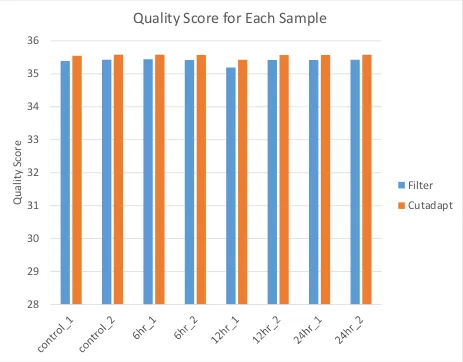
A. Quality Control
The first part of ensuring that the quality for the initial reads and then the alignments
were good involved using FastQC to verify the quality of the samples. This was done after the
samples were filtered using FastX (filter), and the reads less than 50 bp in length were removed
with Cutadapt (cutadapt). FastQC gives a number of different stats and figures for the
determination of quality. The basic stats give a good general summary and enable some basic
comparisons between the samples. However, two important ones for the validation of overall
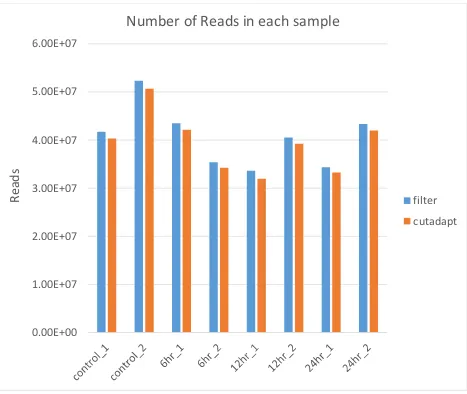
quality are the overall quality score (Figure 3) and the total number of reads (Figure 4). FastQC
gives a quality score of 0-36 with 28-36 being considered good quality scores. As can be seen,
the average quality score, which is calculated from the per sequence quality score, is around 35,
and does not show much change between the filtered and cutadapted scores. Additionally, the
20 change in the number of reads, indicating that removal of the smaller reads did not affect the
overall size of the sample. In other words, the smaller reads were not the majority of the reads in
any of the samples. Based on this, the samples were determined to be of good quality and
[image:26.612.75.538.210.572.2]alignment, and differential analysis was commenced.
Figure 3: Quality Score Comparison:
Comparison between the quality score for the cleaned, sequenced files after quality filtration (filter), and after removal of all reads under 50 bp through the use of cutadapt. The quality scores produced by FastQC are 0-36, with 36 being the best quality, and 28-36 being considered good quality scores. The average quality score for each sample was produced using the data from per sequence quality score data.
28 29 30 31 32 33 34 35 36
Qua
lit
y
Sc
or
e
Quality Score for Each Sample
21
Figure 4: Number of Reads:
Comparison between the read lengths of the cleaned sequenced files, after quality filtration (filter), and after removal of all reads under 50 bp through the use of cutadapt.
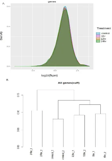
Once alignment and differential analysis were complete, and the cuffdiff files produced,
and being used by CummeRbund, a final quality control check was necessary. There are several
quality metrics that come with the CummeRbund package. We used dispersion plot and the
dendrogram at the gene level (Figure 5) and the csScatterplot (Figure 6). For the dispersion plot,
for good quality data, all treatments must have a normal curve. Ideally, the normal curves would
all be at a similar position. This is what can be seen in Figure 5A. The dendrogram is a check for
the different replicates for each treatment. What is needed when running the dendrogram is to
0.00E+00 1.00E+07 2.00E+07 3.00E+07 4.00E+07 5.00E+07 6.00E+07
R
ead
s
Number of Reads in each sample
22 have the individual replicates for each treatment divide into different groups, which can be seen
in Figure 5B, assuring that the replicates for each treatment are more similar to each other than
they are to any other replicate from another treatment. Additionally, one can see that the 12- and
6-hour treatments are most similar to each other, and that the 24-hour is the most different from
the other treatments, occurring in its own cluster, with just the two 24-hour replicates. For the
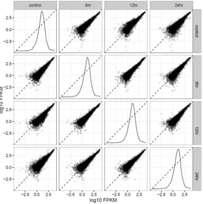
csScatterplot (Figure 6), this gives two quality metrics. First, each scatterplot between two
different treatments should be roughly along the scatterplot regression line, and dispersed along
that line, which can be seen with most of the individual gene values log10(FPKM) following
along the generated regression line. Also, those values are spread out and not in one clump,
indicating good dispersion. In addition, when a scatterplot is done against the same treatment, a
normal curve is produced again. This indicates that the treatments are dispersing correctly. Given
all of these factors, it was determined that that the samples and treatments were of good quality,
23
Figure 5: Differential Analysis Quality Metrics:
A) Dispersion plot at the gene level. A good dispersion is shown by a normal curve for all samples, and normal curves covering roughly the same dispersion range. B) Dendrogram at the gene level. This shows that the replicates divide into different groups, indicating that the
24
Figure 6: Scatterplotmatrix for All Treatments:
This Figure shows that the dispersion is of good quality. First, that the scatterplots between two different treatments result in most of the genes occurring along or relatively close to the line. Second, in the comparison between the same samples, this results in a normal curve.
B. Timepoint Differential Analysis
To understand the overall expression patterns of the RNA-seq data, the significantly
25 timepoint. All these groups will be called the RNA-seq data throughout this paper. The RNA-seq
data was then further divided into two groups: first, those RNA-seq data that have a
corresponding gene in the ChIP-seq datasets that had been previously identified (ChIP-seq genes
or ChIP genes), and second, those that have a corresponding gene with a ChIP-seq site that is
within 5kb of its TSS site (5kb ChIP genes or 5kb ChIP-seq genes). The ChIP genes contain all
the 5kb ChIP genes.
To demonstrate how exposure to 5-fu, and therefore the induction of a stressor and
activation of p53, affected the regulation expression of associated genes (either up or down), the
comparison between timepoints was undertaken. Also, a focus was on the control
(non-treatment) vs the treatments (6-hour, 12-hour and 24-hour). Additionally, already-identified ChIP
genes that had corresponding significantly differentially expressed RNA-seq genes were
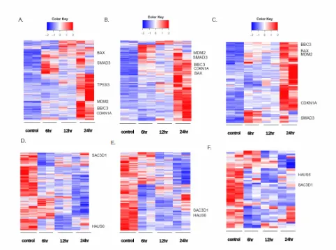
investigated. Figure 7 A, B, and C are heatmaps showing the significantly differentially
upregulated genes (for both replicates) at all timepoints. Figure 7A is a heatmap of all the
significantly differentially expressed RNA-seq genes (although these are not necessarily protein
coding), Figure 7B is all previously-identified ChIP-seq genes in our dataset [19] [20] [7] that are
also significantly differentially expressed RNA-seq genes, and Figure 7C is all
previously-identified ChIP-seq 5kb genes (where the ChIP-seq site and the TSS site are within 5 kb of each
other), and are also significantly differentially expressed RNA-seq genes. Figure 7D shows the
downregulated RNA-seq genes. Figure 7E is the downregulated ChIP genes, and Figure 7F
shows the 5kb ChIP genes that are downregulated.
As can be seen in all heatmaps, there is a reversal between the control (0hr) and 24hr,
with mostly high amounts in the upregulated heatmaps for 24 hours, and mostly low amounts for
26 high expression for 6 hours in both the up and downregulated heatmaps. However, one should
keep in mind that a gene could be differentially upregulated in 6 hours, and the 24 hours be
differentially expressed enough higher from the 6-hour that it would appear that the 6-hour gene
is at the same or similar level of expression compared to the control when the two timepoints are
differentially expressed.
To show differences in sorting, and where particular genes occur for upregulated genes
(7A, 7B and 7C) CDKN1A, BBC3, BAX, TP53I3, SMAD3 and MDM2 were used as indicators.
While CDKN1A, BBC3, BAX, MDM2 and SMAD3 occur in all sets (RNA-seq, ChIP genes,
5kb ChIP genes), TP53I3 does not. This is particularly interesting with TP53I3, due to the fact
that it is highly differentially expressed. Additionally, while CDKN1A, BBC3 and TP53I3
appear to upregulated only at 24 hour, they are actually upregulated compared to the control in
all the treatments. Considering how easy it is to find this within commonly p53-associated genes,
care should be taken not to discount that earlier hours might also be upregulated, just not to the
same level as 24 hours.
To demonstrate similarly, the difference in patterns in each heatmap sorting HAUS6 and
SAC3D1 were used. Both were found in the 5kb gene downregulated dataset. It is also
noticeable that HAUS6 is downregulated at 12 hours, while SAC3D1 is downregulated
significantly at 6 hours and 12 hours, but not 24 hours, putting it in one of the areas where there
is not an expression difference between control and 24 hours, which there appears to be
relatively more of in Figure 7F.
27
Figure 7: Heatmaps:
All are significant RNA-seq genes q<0.05 A) Significant upregulated RNA-seq has 2794 genes. B) Significant upregulated ChIP-seq genes in RNA-seq dataset has 524 genes. C) Significant upregulated ChIP-seq genes within 5kb of TSS site that correspond to RNA-seq dataset has 123 genes. D) Significant downregulated RNA-seq has 3425 genes. E) Significant upregulated ChIP-seq genes in RNA-ChIP-seq dataset has 511 genes. F) Significant upregulated ChIP-ChIP-seq genes within 5kb of TSS site that correspond to RNA-seq dataset has 53 genes. See discussion for how each dataset was determined.
Another way of understanding this is to look at the overall significant genes for each
timepoint. To this end, the significant genes were examined in two ways. Since the
non-treatment (control) vs a non-treatment time was of particular interest, the up and down significant
28 significant differential expression, are found in these 3 sets. The venn diagrams between these
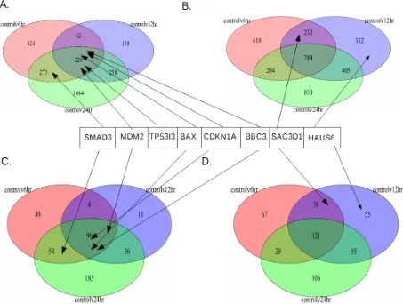
sets were produced (Figures 8 and 9).
For both Figures 8 and 9 A and B are the RNA-seq differential expression for
upregulated compared to control (Figure 8A and 9A), and downregulated compared to control
(Figures 8B and 9B). As can be noted, all the genes of interest are the same set as in Figure 7. As
with the Figure 7, SMAD6, MDM2, TP53I3, CDKN1A, BBC3 and BAX are all upregulated and
SAC3D1 and HAUS6 are downregulated (Figure 8 and Figure 9). It can also be noted that
MDM2, TP53I3, CDKN1A, BBC3 and BAX are upregulated at all timepoints compared to the
control (Figure 8A and Figure 9A). Also, as with the heatmaps, TP53I3 does not occur in the
ChIP genes subsets (Figure 8C and Figure 9C). SMAD6, on the other hand, is the only
upregulated gene that does not occur at all three timepoints. It is upregulated at only 6 and 24
hours (Figures 8A, 8C, 9A, and 9C).
Finally, SAC3D1 and HAUS6 are not downregulated at 24 hours; instead, they are
downregulated at6 hours and 12 hours for SAC3D1, and 12 hours for HAUS6. Additionally, of
the genes that are up or downregulated individually, 24-hour has the most for up and
downregulated, with more for upregulated genes. The same is seen for ChIP-seq differential
expressed genes (Figure 8 C and D), which has more genes overall when compared with both the
full ChIP RNA-seq intersection or the 5kb ChIP-seq differentially expressed gene (Figure 9 C
and D). This is not to say that genes occurring at 24 hours are not also differentially expressed at
other timepoints. While 24 hours has the largest number of individual genes, of the total genes
upregulated at 24 hours, between 44-67% are also upregulated at other timepoints.
For 6 hours for RNA-seq (Figures 8 A&B and 9 A&B), up and downregulated are
29 are more downregulated genes for all ChIP RNA-seq compared to upregulated (Figure 8 C&D).
Conversely, for 12 hours, there are more downregulated genes compared with upregulated, and
this holds true for the full differentially expressed RNA-seq dataset, as well as the ChIP subsets.
Additionally, for the 5kb ChIP upregulated genes, control vs 12-hour does not have any genes
that are not upregulated at either control vs 6-hour or control vs 24-hour. Furthermore, for all
upregulated sets, control vs 24-hour has the highest number of upregulated genes that do not
intersect with any other sets. This is the same for RNA-seq and ChIP downregulated genes, but
30
Figure 8: Venn Diagrams for RNA-seq and ChIP Genes:
31
Figure 9: Venn Diagrams for RNA-seq and 5kb ChIP Genes:
Shows the up and downregulated number of genes compared to the control for each treatment timepoint, and which timepoints those genes intersect, along with where SMAD3, MDM2, TP53I3, CDKN1A, BBC3, SAC3D1 and HAUS6 occur. A) RNA-seq up. B) 5kb ChIP genes up. C) RNA-seq down. D) 5kb ChIP genes down. RNA-seq are all the significant differentially
expressed RNA-seq genes at each timepoint, while 5kb ChIP genes are the RNA-seq differentially expressed genes that correspond to ChiP-seq sites within 5kb of their TSS site.
Finally, the numbers for differential expression for treatment and all the treatments were
computed, along with the number of protein coding genes for up and downregulation. As can be
seen in Figure 10, overall there are more down differentially expressed genes than up
differentially expressed genes for 6 hours and 24 hours. The converse is true for the control, but,
given an upregulated control gene must have a downregulated gene at another timepoint, this
32 subset, the numbers are close between down and upregulation, but there are more upregulated.
However, when one looks at the differentially expressed genes for 24 hours (Figure 10E), there
are more upregulated genes than there are downregulated genes. Additionally, the difference
between the up and downregulated genes is smaller for 24 hours than it is for the other
[image:38.612.95.518.252.522.2]treatments. A similar pattern is observed for the up and downregulated coding genes.
Figure 10: Protein Coding and All Genes, Regulation by Timepoint:
33
C. Non-protein Coding RNA
To further investigate the differentially expressed RNA that is not a protein coding gene,
and to investigate non-protein coding RNA that has been associated with p53 in previous studies
(such as [7]), we used already identified lincRNA, miRNA and ERV1 elements. For linRNA and
miRNA, these were from publicly-available datasets found at the UCSC Genome Browser, with
some modification (see materials and methods section). An intersection was then preformed both
ways between the RNA-seq significant genes and RNA elements of interest, or between RNA
elements of interest and significant RNA-seq genes. The results of the treatment series
breakdown can be seen in Figures 11 and 12. For these elements, miRNAs have the largest
number of intersections, with the larger number occurring in downregulated genes (except for the
control, but again an upregulated control indicates a downregulated treatment), which is reversed
in the 5 kb RNA-seq ChIP genes, possibly due to the 5kb selection. ERV1 is the same as
miRNA. However, lincRNA is reversed, with more upregulated genes intersecting with lincRNA
at 24 hours, which was not seen for the other timepoints. This could be due to the selection for
non-coding genes that occur for the lincRNA. Interestingly, there appear to be more than one
RNA element intersection with a number of RNA-seq. This could be due to biologically different
elements, or two elements with different names that occupy the same or very similar locations.
This can be seen in Figure 13A and Figure 15A and 15C, which is more prevalent and will
34
Figure 11: Non-coding RNA Genes Regulation by Timepoint:
Up and downregulated genes at each timepoint that intersect with either lincRNA, ERV1/LTR, or miRNA. A) Control intersections. B) 6-hour intersections. C) 12-hour intersections. D) 24-hour intersections. The genes are the RNA-seq genes that are significantly differently expressed. ChIP genes are the subset of RNA-seq genes that also occur in the ChIP-seq dataset previously
35
Figure 12: Non-coding Intersections per Timepoint:
Up and downregulated RNA-seq genes of which lincRNA, ERV1/LTR, and miRNA have an intersection. A) Control intersections. B) 6-hour. C) 12-hour intersections. D) 24-hour
intersections. The genes are the RNA-seq genes that are significantly differently expressed. ChIP genes are the subset of RNA-seq genes that also occur in the ChIP-seq dataset previously
produced. The 5kb ChIP genes are the subset of the ChIP genes that also are within 5kb of their TSS site.
D. Expression and Imaging.
To better illustrate expression, and to show that no treatment had replicates with widely
varying counts, several genes of interest were imaged using the IGV browser. In addition to the
tracks for each one, sample tracks were used from the ref-seq (NCBI database), miRNA, ERV1
and lincRNA and the ChIP-seq sites. This enabled viewing of the expression at any particular
36 Figure 13 is a comparison between CDKN1A (13A and 13C) and TP53I3 (13B and 13D).
TP53I3, while it has not been identified in our previously processed ChIP-seq data [32], it had
been noted previously as having a large increase in expression when compared to 12 and 6 hours
of treatment [45]. The same thing is seen here as can be seen in 13B and 13D. Twenty-four hours
is much more expressed than 6 hours. However, it should be noted that even though 6 hours
appears to be similar in expression to 6 and 12 hours, both of those timepoints are also
significantly upregulated when compared to the control. Comparatively, with CDKN1A 13A and
13C, while there is a difference between 6 hours and 12 hours and 24 hours, there is again an
increase at 24 hours. It is visually clear that there was also an increase at 6 and 12 hours when
compared to the control.
Figure 14 is a comparison between BBC3 and BAX, two other genes that have been
associated with p53. As can be seen, BBC3 (Figure 14A and 14C) has a similar pattern to
CDKN1A: an initial increase in expression at 6 hours, with 12 hours being similar in expression,
followed by another, larger, increase in expression at 24 hours. BAX, however, doesn’t have that
jump in expression seen at 24 hours in the other 3 genes to varying degrees. Instead, it has a slow
increase in expression that does not result in any significantly different expression between the
treatment timepoints (6hr, 12hr, 24hr).
It was noted that SMAD3 (Figure 15) is one of the subset of 5kb ChIP genes that appear
visually to be upregulated at 6 hours. Because of this, and due to the fact that it has been shown
that SMAD3 in response to TGEF-β signaling induces BBC3 [46], we investigated SMAD3.
Additionally, SMAD3 has been found to complex FOXO genes in response to TGEF-β
signaling, and that the complex of FOXO genes and the SMAD3 gene results in the induction
37 associate with MDM2’s second promoter region, resulting in an increase in the already increased
MDM2’s expression [48]. This is on top of the induction that has been shown to occur via p53
directly, even though MDM2 is the main repressor of p53 results through the degradation of the
p53 protein [49].
First, it should be noted when looking at SMAD3’s IGV plot (Figure 15A), that is hard to
visually see any real difference between the control and 6 hours or 24 hours (the treatment times
where SMAD3 is differentially expressed). Also of note is that the FPKM values are lower than
seen in Figure 13 or Figure 14 for SMAD3 (Figure 15C). MDM2, on the other hand, is a
different story, with high with FPKM values similar to the FPKM values (Figure 15D) of BAX,
BBC3, and TP53I3 (Figure 13D, Figure 14C and Figure 14D). With the IGV plot, it is also
visually obvious that there is a difference between the control and all treatment timepoints, and
between 12-hour and 24-hour. What is very interesting is that that both SMAD3 and MDM2
have extremely similar expression patterns (Figure 15C and Figure 15D). The expression pattern
is this: an increase in expression at 6 hours, followed by a reduction at 12 hours, and then another
increase at 24 hours, coinciding with the second much larger increase in expression observed in
this study.
HAUS1 and SAC3D1 (Figure 16) are examples of downregulated genes. In other words,
the control has higher expression than at least one of the treatment timepoints, and none of the
treatments have a higher expression than the control. Several interesting observations can be
noted. First, compared to the expression range for the upregulated genes, both HAUS1 and
SAC3D1 have a lower maximum in the tens instead of the hundreds for FPKM (16C, 16D, 14C,
14D, 13C and 13D). The results in the lower count seen on the IGV plots as well (16A and 16B).
38 as seen in genes upregulated specially in the p53 cycle. Second, there isn’t that large jump
between treatments. This results in treatments in other than 24-hour differentially expressed
timepoints. One explanation, particularly when taking 7D and 7E into account (which have much
less 24-hour clear downregulation), is that 5kb ChIP sites for downregulated genes are rare—a
total of 53 genes—which might be the result of p53 not directly downregulating genes.
GAPDH is a housekeeping gene and to assure that the differential expression seen is not
due to possible other factors a housekeeping gene (GAPDH) was examined Figure 17. Despite
what appears to be an increase in the FPKM value at 12 hours (Figure 17B) all of the timepoints
are not differentially expressed from one another. The IGV plot shows this more clearly, with the
expression quite clearly being very similar between all of the samples (Figure 17A).
Additionally, GAPDH has the largest counts and FKPM values of any of the genes of interest
looked at in this study, demonstrating how common GAPDH expression is. This gives support
that the differential expression observed in the RNA-seq data is due to actual biological effects
and not effects of sample differences that effected expression overall.
For each lincRNA, miRNA and ERV1, one RNA-seq gene that they had intersected with
was chosen for demonstration purposes (Figure 18). Two things are immediately clear. The
expression count levels are lower than the genes of interest, and the increase pattern seen in the
genes strongly associated with the p53 pathway are not observed. For the lincRNAs (Figure
16A), instead of expression increasing vs the control, there is a decrease (downregulation)
compared to the control. However, as with Figure 13, all of the replicates are similar to each
other for each treatment. In addition, for one of the lincRNA tracks there are two lincRNAs at
almost identical locations. There is only one timepoint with difference in expression from the
39 timepoint. In this case, there is only one miRNA which can be seen in both the Ref-seq track and
the miRNA track. ERV1 (Figure 18C) is interesting. First there are, again, two ERV1 RNAs at
basically the same location. Second, the expression pattern is interesting. At 6 hours, there is an
increase in expression compared to the control, followed by a decrease in expression, and then
the same increase again at 24 hours, possibly due to a second induction or increase of p53 at 24
hours. The downregulation for both lincRNA and miRNA makes sense due to the overall larger
40
Figure 13: Expression of CDKN1A and TP53I3:
41
Figure 14: Expression of BBC3 and BAX:
Charts the expression as shown through the IGV browser, and through expression plots which show the error bars for each treatment. A) BBC3 IGV plot, B) BAX IGV plot, C) BBC3
42
Figure 15: Expression of SMAD3 and MDM2:
43
Figure 16: Expression of HAUS6 and SAC3D1:
44
Figure 17: Expression GAPDH
45
Figure 18: Expression of Non-coding RNA Examples:
Charts the expression as shown through the IGV browser for lincRNA, miRNA, ERV1 expression examples. A) lincRNA. B) miRNA. C) ERV1.
46 GO terms can give an idea of areas of increase between treatments to show what
biological processes may have become active. To this end, the top significant terms for each
treatment and ChIP association were plotted in Figure 19, and, since the descriptions for the
terms where very long, abbreviations were used, and full terms can be found in Figure 20. As can
be seen, many of the biological processes terms with significant (q<0.05) fold increases are
related to either the cell cycle or apoptosis. In fact, the term with the highest fold increase is
“DNA damage response, signal transduction by p53 class mediator resulting in cell cycle arrest,”
which relates directly to p53. This again is another validation that p53 was active, and the
differences that have been observed in the RNA-seq data is a result of the activation of the p53
cycle. Additionally, ChIP genes, particularly those within 5kb of a TSS site, tend to be more
associated with apoptosis and have a higher fold enrichment value. This could be due to the
selection that occurs with only taking genes that can be found through ChIP and those that are
47
Figure 19: GO Biological Term Fold Enrichment Top Significant Terms:
48
Figure 20: GO Terms Full Descriptions:
Gives the abbreviated terms used in Figure 19, and the full term description associated with that term.
F. ChIP-qPCR.
To determine whether the common pattern seen in the RNA-seq data could be observed
with ChIP data, an initial ChIP-seq experiment was run using the same treatment and control
conditions. Following the immunoprecipitation, the % input was calculated for replicates 1 and
2 of the control and 24-hour treatment, and replicate 1 of the 6- and 12-hour treatments. As can
be seen in Figure 21, the ChIP, which shows the protein interactions with the chromatin, shows a
49 21, both the negative and positive primers are at low percentages, indicating that there isn’t a
large amount of non-specific binding of our antibody. Additionally, the same pattern that was
observed for both BBC3 and CDKN1A, and overall for the RNA-seq data, was observed: an
initial increase in % input at 6 hours, and reduction in the % input at 12 hours, and a much larger
increase in % input at 24 hours. This validates that the pattern seen in the RNA-seq data is also
seen in the protein chromatin interaction, and that it is a real biological effect of 5-FU induced
50
Figure 21: ChIP qPCR of p53 target genes:
Shows the % input of two genes of interest that have been shown to be upregulated by p53 with our RNA-seq data BBC3 and CDKN1A. The pattern of % input increase is similar to what was observed in RNA-seq data validating the pattern observed.
V. Conclusions
This study focused on RNA-seq data for p53 activation via the drug 5-FU for 6 hours, 12
hours, and 24 hours, along with the non-treatment control, and the comparison between those
timepoints, plus a selection of RNA-seq identified genes that have also been identified in 0% 1% 2% 3% 4% 5% 6% 7% 8% 9%
control control 2 6hr_1 12hr_1 24hr_1 24hr_2
% in
p
u
t
5-FU treatment
ChIP qPCR of p53 target genes
positve
negative
BBC3
51 previous ChIP-seq studies. One of the things that has been noted in a number of different
instances is that at 6 hours there is an initial induction of genes, and at 24 hours there seems to a
further induction of the same genes. This can be seen in Figure 13 and Figure 14, where, on the
expression plots for CDKN1A (13C) and BBC3 (14C), there is an initial upregulation at 6 hours,
with 12 hours having an upregulation similar to 6 hours, and then a further noticeable increase in
expression at 24 hours. This pattern has also been observed in initial ChIP-seq % input qPCR
results from the same treatment conditions and cells which show a similar pattern that has been
observed from the RNA-seq results (Figure 21).
Several genes have been shown to be upregulated at 6 hours and again at 24 hours, but
have the appearance on heatmaps of only being induced at 24 hours. This is particularly true with
TP53I3 (13D). When just examining visual representations of expression among all 4 timepoints,
this increase in regulation can look as if there is no increase between 6 hours and the control. For
most genes in the data, when a gene is upregulated, it is either induced at 24 hours, or induced at
6 or 12 hours, and then further induced at 24 hours. This explains why the increase in expression
is clear for 24 hours in Figures 7A, 7B and 7C, but is only seen for a subset of the 6-hour genes.
For example, CDKN1A on Figure 7C is upregulated compared to the control at 6, 12, and 24
hours, but it is only visible at 24 hours because of how much larger the increase in expression
was at 24 hours. Therefore, stating that there are more genes induced later, at 24 hours, compared
to earlier at 6 hours, is based purely on the expression patterns. However, what is observed in
Figure 8 and Figure 9 is this: there are a number of genes which are upregulated at all timepoints.
Again, between 44-67% of the control vs 24-hour genes are also induced at other timepoints,
with increasing percentages in the ChiP gene subsets. Bottom line, there is a large increase in