Search space pruning and global optimization of multiple gravity assist trajectories with deep space manoeuvers

Becerra, V.M. and Nasuto, S.J. and Anderson, J.D. and Ceriotti, M. and Bombardelli, C. (2007)

Search space pruning and global optimization of multiple gravity assist trajectories with deep

space manoeuvers. In: IEEE Congress on Evolutionary Computation (CEC), 25-28 September 2007,

Singapore.

http://

strathprints

.strath.ac.uk/

20156

/

Strathprints is designed to allow users to access the research output of the University

of Strathclyde. Copyright © and Moral Rights for the papers on this site are retained

by the individual authors and/or other copyright owners. You may not engage in

further distribution of the material for any profitmaking activities or any commercial

gain. You may freely distribute both the url (

http://

strathprints

.strath.ac.uk

) and the

content of this paper for research or study, educational, or not-for-profit purposes

without prior permission or charge. You may freely distribute the url

(

http://

strathprints

.strath.ac.uk

) of the Strathprints website.

Search Space Pruning and Global Optimization of Multiple Gravity

Assist Trajectories with Deep Space Manoeuvres

V.M. Becerra, S.J. Nasuto, J. Anderson, M. Ceriotti and C. Bombardelli

Abstract— This paper deals with the design of optimal mul-tiple gravity assist trajectories with deep space manoeuvres. A pruning method which considers the sequential nature of the problem is presented. The method locates feasible vectors using local optimization and applies a clustering algorithm to find reduced bounding boxes which can be used in a subsequent optimization step. Since multiple local minima remain within the pruned search space, the use of a global optimization method, such as Differential Evolution, is suggested for finding solutions which are likely to be close to the global optimum. Two case studies are presented.

I. INTRODUCTION

A gravity assist manoeuvre uses a celestial object’s gravity in order to change a spacecraft’s trajectory. When a space-craft approaches a celestial object, a small amount of the object’s orbital momentum is transferred to the spacecraft. This manoeuvre was used for the first time in the 1970’s, when the spacecraft Mariner 10 used a gravity assist fly-bys of Venus to reach Mercury. Gravity assist manoeuvres (GAs) are frequently used to reduce fuel requirements. Most interplanetary trajectory design problems can be stated as optimization problems, where one of the fundamental goals is the minimization of fuel requirements, with consideration also given to intermediate planetary flybys, mission duration, type of arrival, launch and arrival windows, and velocity constraints. Traditionally, local optimization has been used to attempt to solve these design problems [1]. However, because of nonlinearities and the periodic motion of the planets, multiple local minima exist and, as a result, local optimization only helps to find local minima which are heavily dependent on the initial guesses employed and are not necessarily good solutions. The use of global optimization techniques has been proposed for tackling these problems, as these methods have a better chance of finding good solutions approaching the global optimum [2]. Genetic algorithms and similar techniques have been employed, but these techniques may face difficulties in tackling realistic missions due to the large size of the search space associated with these problems. A method known as GASP (Gravity Assist Space Pruning) has been proposed [3] in relation with problem of multiple gravity assist (MGA) trajectories with a known planetary sequence and no deep space manoeuvres. In such cases, it can be shown that the vast majority of the search

V.M. Becerra, S.J. Nasuto and J. Anderson are with the School of Systems Engineering, University of Reading, UK, (phone: +44-118-3786703 fax: +44-118-3788220; email: [email protected]). M. Ceriotti is with the Department of Aerospace Engineering, University of Glasgow, UK. C. Bombardelli is with the Advanced Concepts Team, European Space Agency, Noordwijk, the Netherlands

space consists of infeasible, or very undesirable, solutions. This observation motivated the development of a method for producing reduced search spaces by pruning, thus allowing standard global optimization techniques to be applied more successfully to the reduced box bounds. The GASP method considers the sequential nature of the problem, as it prunes the search space on a phase by phase basis, and results in important computational savings, with search space reduc-tions greater than six orders of magnitude, thus simplifying significantly the subsequent optimization. The method is based on grid sampling in two dimensions for each leg of the mission, with sequential pruning of the search space. The pruning method has been shown to have polynomial time and space complexity, so that it remains tractable as the number of decision variables increases. However, designing multiple gravity assist missions with no deep-space manoeuvres is limited in scope, since many possible trajectories cannot be considered, and, as practice shows, deep space manoeu-vres are used in real missions. If the problem of multiple gravity assist with deep space manoeuvres could be pruned efficiently, then the computational cost of optimizing such trajectories may be significantly reduced. The introduction of deep space manoeuvres offers the further advantage of providing a reasonable approximation of multiple gravity assist trajectories with low-thrust arcs. If a transfer arc is no more simply ballistic but is shaped by one or more propelled manoeuvres (either impulsive or low-thrust) the number of degrees of freedom increases significantly. Hence, an efficient solution process would have to make use of additional information to reduce the number of possible alternatives (pruning the search space) so reducing the computational cost, and increasing the likelihood of finding good solutions. This paper describes a method for pruning of the search space of multiple gravity assist optimization problems with deep space manoeuvres, for the particular case of powered swingbys. The method can be seen as an extension of the GASP method when deep space manoeuvres are considered. Since the pruned problem would still exhibit multiple local minima, the use of a global optimization method to find optimal solutions on the pruned space is proposed.

II. GENERAL PROBLEM FORMULATION

The problem of interest may be formulated as a multi-stage optimization problem (MSOP).

MSOP:Find

x= xT

1, xT1, · · ·, xTs+1

T

to minimise

f(x,z1, . . . ,zs+1)

subject to

zk=hk(x1, . . . ,xk+1), k= 1, . . . , s

gk(zk)≤0, k= 1, . . . , s+ 1

Ωis the Cartesian product of s+1 hyper-rectanglesΩ = Ω1×

Ω1× · · · ×Ωs+1, where Ωk = {xk ∈ Rnk|x

(k)

L ≤ xk ≤

x(k)

U }, k = 1. . . , s+ 1, the objective function is assumed

to be scalar f : Ω×Rq1 × · · · ×_Rq_{s+1 →}

R, the vectors

zk∈Rqk,k=1,. . . ,s+1, are intermediate variables associated

with each stage, and each of the functions hk : Ω1×Ω2×

· · · ×Ωk+1→Rmkandgk: Rqk→Rdkis associated with a

particular stagek. Note that the calculation of the constraint function gk depends on intermediate variables calculated at

stagek, and the objective function depends on the values of the intermediate variableszk,k=1,. . . ,s+ 1, hence a specific

order must be followed to evaluate the objective functionf and the constraint functionsgk.

The presence of inequality constraints in the MSOP re-quires careful consideration. Although bounds on the deci-sion variables are easy to manage, more general inequality constraints are more difficult to handle in global optimiza-tion. A plausible method is to prune the search space based on feasibility (i.e. constraint satisfaction). This has an important benefit: the size of the search space is reduced hence simplifying the optimization task. One simple method of pruning is to grid sample the search space with a suitable resolution so that unfeasible areas can be detected by evalu-ating the constraint functions, and subsequently eliminated, leaving a reduced search space where optimisation can be applied. However, the cost of grid sampling with reasonable resolutions may be prohibitive when the search space dimen-sion is larger than two or three.

The mission considered by the GASP method includes powered gravity assist at intermediate planets, and if required a braking manoeuvre at the arrival planet for orbit insertion. The problem addressed by GASP can be cast as a MSOP. Here, the decision vectorx consists of the launch date and transfer times between planets, the intermediate variableszk

are the ∆v’s applied at each planet. The functionshk

repre-sent the calculations that are required to find the intermediate variables (solution of Lambert problems, swing-by models), the objective function is the sum of the magnitudes of the ∆v’s. The constraint functionsgkare related to upper bounds

on the∆v’s at each planet (as thrusters have limits), as well as lower bounds for the periapsis radius at each swing-by planet (to keep a safe distance from the planet).

III. MODELLING A MISSION LEG WITH DEEP SPACE MANOEUVRES

We have used a model that is able to compute the trajectory from one planet to the next planet in a mission, with an ar-bitrary number of intermediate deep space manoeuvres. The model requires specifying the initial and final positions of the spacecraft, the time of flightTofbetween the planets, and

the positions and the timing of all deep space manoeuvres involved, and it returns the velocity vectors at the begining and at the end of the leg, together with the magnitudes of the deep space impulsive manoeuvres.

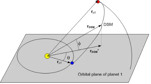
With reference to Figure 1, the initial position of the spacecraft, rp1 can be found by an ephemeris calculation

related to the initial planet given the departure date t0.

Similarly, the final position of the spacecraft rp2 can be

found by an ephemeris calculation related to the next planet, given the arrival timetarr, which can be calculated astarr = t0+Tof.

Fig. 1. Mission leg model with a deep space manoeuvre

Each deep space manoeuvre is characterized in polar co-ordinates with the following parameters:

• r: dimensionless distance from the sun. The vector from the sun to the deep space manoeuvre is denoted as

rDSM. The value r is equal to zero when |rDSM| is equal to|rp1|, andris equal to 1 when|rDSM|is equal

to|rp2|. Notice thatrmay be outside the interval [0,1]

when the orbits of the planets are eccentric.

• θ: in-plane angle (angle betweenrp1and the projection

of rDSM on the orbital plane of the first planet). This

projection is denoted as rDSM in Figure 1.

• φ: out of plane angle (angle between rDSM and the projection of rDSM on the orbital plane of the first planet)

In addition, the timing of the deep space manoeuvre is parameterized as a fraction α ∈ [0,1] of the time of flight, such that the timing of the deep space manoeuvre is expressed as α×Tof.

In the model, a patched conic, two-body problem is considered. The manoeuvres are assumed to be impulsive. In case of a single deep space manoeuvre, then the leg trajectory is found through the solution of two Lambert problems. We used an implementation of Battin’s method for the Lambert solution. See [4], [5] for further details on the algorithms involved.

final velocities are outputs from the Lambert solver. Once two consecutive legs are computed, both the incoming and outgoing velocity at the planet become available and the swingby (with the powered model) can be computed.

In this way, in order to create the whole trajectory, the only requirement is that the time at each planet is the same for all the phases arriving or departing from that planet. At this point, no constraints are considered on the incoming and outgoing velocities. Thus, it is possible to analyze (optimize, prune) the deep space flight phases first, then match them with the swingbys and prune again on the basis of the feasibility of the swingby.

This approach is not possible with a model of swingby which in some way computes the outgoing velocity, because in this case, it would be necessary to match both time and velocity in order to combine deep space flight phases with swingby phases.

IV. MODELLING A POWERED SWINGBY

The gravity assist calculations consist of matching the incoming and outgoing planetocentric velocities around the swingby planet, and computing a minimum passing distance, which is also known as the pericenter radius. If the pericenter radius is unacceptably low, it is possible to calculate a suitable velocity impulse to be applied to achieve a minimum desired altitude. When the manoeuvre requires such an impulse, it is known as powered swingby. A gravity assist manoeuvre is illustrated in Figure 2.

Thrust

applied

here

V

r

Planet

Spacecraft

trajectory

Hyperbolic

asymptote

Hyperbolic

asymptote

Fig. 2. Illustration of a gravity assist manoeuvre

The gravity assist model takes the planetocentric incoming and outgoing velocities, the minimum pericenter radius, and the gravitational constant of the planet, and returns the required impulsive∆v [4].

V. THEGASPALGORITHM WITH POWERED SWINGBYS AND DEEP SPACE MANOEUVRES

Inspired by the original GASP algorithm, its extension considering deep space manoeuvres and powered swingbys described in this section, also prunes the search space con-sidering each phase of the mission in a sequential manner. The introduction of a deep space manoeuvres increases significantly the number of decision variables.

In order to keep the description of the method simple, we consider a two phase mission with one deep space manoeuvre at each phase, and one gravity assist manoeuvre. We also assume that a braking manoeuvre is performed for orbit insertion purposes at the arrival planet [6]. The method can be extended to more phases and more deep space manoeuvres per phase in a straightforward manner.

The notation used below is as follows. The super-index in parenthesis (e.g.(1),(2)). indicates the phase of the mission. ∆vdep is the impulsive manoeuvre at departure,∆vDSM is

an impulsive manoeuvre at deep space,∆vgais an impulsive

manoeuvre at a gravity assist planet, ∆vb is a braking

manoeuvre that is performed for orbit insertion purposes,

vin is the arrival velocity at a swingby planet, vout is the

departure velocity from a swingby planet, t0 is the mission

launch date, tarr is an arrival time at the end of one phase, tdepis the departure time at the beginning of a phase,Tof is

the time of flight of a given phase.

A. First phase

The decision vector associated with this leg is as follows:

x1= [t0, T (1)

of , r

(1)_{, α}(1)_{, θ}(1)_{, φ}(1)

]T (1)

In contrast to the original GASP algorithm, where there are only two decision variables (t0, T

(1)

of ) associated with

the first leg, there are now six decision variables associated with the first leg. The threefold increase in the number of decision variables makes it too expensive to carry out a grid sampling, as is shown in the first case study below.

Assume thatx1 is initially limited to the hyper-rectangle Ω1⊂ 6, such that each element of x1 is initially bounded

between lower and upper limits: xl

1,j ≤ x1,j ≤ xu1,j, j =

1, . . . ,6.

We are interested in pruning the search space by finding an estimate of the feasible regions of the search space associated with the first leg, with respect to constraints on the departure impulse ∆vdep(1), and the deep space manoeuvre impulse

∆v(1)DSM. To find such an estimate, we propose the use of

a local optimization algorithm, which can be started from multiple random vectors within the admissible regionΩ1, and

Algorithm 1: Pruning the first phase:

1) Generate randomly N1 starting vectors within the

admissible region for the first phase: x¯i

1 ∈Ω1 ⊂ 6, i= 1, . . . , N1.

2) Start a constrained local optimization algorithm, such as sequential quadratic programming, from each initial vector x¯i1, i = 1, . . . , N1 to solve the following

problem:

min_x

1 f1(x1) = ∆v

(1) dep+ ∆v

(1)

DSM (2)

subject to

∆vdep(1)

∆vDSM(1)

=h1(x1)

∆vdep(1) ≤∆v max dep

∆vDSM(1) ≤∆v max DSM

(3)

where ∆v(1)dep is the impulsive manoeuvre at launch,

∆vDSM(1) is the impulsive manoeuvre performed at deep

space during phase 1. Note that the constrained op-timization algorithm may be stopped as soon as a feasible vector satisfying the inequality constraints is found. If a feasible vector is found, it is recorded as ˆ

xi

1. If no feasible vector is found starting fromx¯i1, then

the optimization starts again with the next value ofi. This step ends with a collection of feasible vectorsxˆi

1 i= 1, . . . , M1, whereM1≤N1. If no feasible vectors

are found, the algorithm stops.

3) Given the set of feasible vector found in step 2, run the clustering algorithm to find a set ofP1 clusters, so

that each vectorxˆi

1 is assigned to a cluster Cj, where

i= 1, . . . , M1 andj= 1, . . . , P1.

4) This step uses the information in the clusters to form one bounding box for each clusterCj,j= 1, . . . , P1.

Letxmin,j_∈ 6_{be a vector so that each of its elements} xmin,j

i is the minimum i-th coordinate value for all

the vectors in cluster Cj. Similarly, let xmax,j ∈ 6

be a vector so that each of its elementsxmaxi ,j is the

maximum i-th coordinate value for all the vectors in cluster Cj. Then the bounding box for cluster j is

defined as

B(1)

j ={x∈Ω1⊂ 6|xmin,j≤x≤xmax,j}. (4)

Note that eachB(1)j is a subset of Ω1, the original search

space for the decision variables associated with phase 1. The set of bounding boxes Bj(1), j = 1, . . . , P1 represents the

initially pruned search space for phase 1 (this set is updated later, in a backward constraining step). Denote B(1) _{as the}

set of bounding boxesBj, j= 1, . . . , P1.

B. Second phase

We are using the patched conic approach to model the trajectory, so that the time of arrival at the end of the first phase is identical to the time of departure for the second phase. In other words, it is assumed that the gravity assist

manoeuvre occurs instantaneously. We have found reduced bounding boxesBj(1), j= 1, ...P1 for the decision variables

associated with phase 1.

Given values for the launch timet0 and the time of flight

for the first legTof(1), the time of arrival at the end of phase

1, which is equal to the time of departure for phase 2, is given by:

t(1) arr=t

(2)

dep=t0+T (1)

of (5)

We have found in phase 1 a set of intervals of feasible values for the arrival time t(1)arr. Such intervals are derived

from the first two co-ordinates of the bounding boxes for phase 1, Bj(1), j = 1, . . . , P1. Since t

(1) arr = t

(2)

dep then it

only makes sense to consider values oft(2)_depwithin the same intervals. This was the main idea that was exploited in the design of the original GASP method [3]. Let us denote the feasible intervals fort(2)depasIj, j= 1, . . . , P1. Note that such

intervals may, in general, overlap. DenoteI as the union of all intervals Ij,j= 1, . . . , P1.

Given that we are assuming a powered swingby, the arrival and departure velocities are decoupled (the departure velocity does not depend on the arrival velocity, provided any bound constraints on the ∆v magnitude are not hit), so we can compute the second phase without having computed first the powered swingby. Assume that the second phase also involves a single deep space manoeuvre, so that the decision vector for the second phase is:

x2= [Tof(2), r

(2)_{, α}(2)_{, θ}(2)_{, φ}(2)

]T (6)

whereT_of(2) represents the time of flight for the second leg, and{r(2)_{, α}(2)_{, θ}(2)_{, φ}(2)_{}are parameters associated with the}

deep space manoeuvre that takes place in the second phase. Let us denote the initial admissible region for x2 asΩ2.

In order to compute the second phase, it is necessary to specify values for t(2)_dep andx2. Define an augmented vector associated with the second phase as follows:

X(2) = [t(2)dep,x

T

2]

T _∈ 6

(7)

Let us define the admissible region for this vector asΩ¯2=

I ×Ω2.

We can formulate the pruning algorithm for the second phase as follows.

Algorithm 2: Pruning the second phase:

1) Generate randomlyN2 starting vectors within the

ad-missible region for the second phase:X¯i

2∈Ω¯2⊂ 6, i= 1, . . . , N2.

2) Start a constrained local optimization algorithm, such as sequential quadratic programming, from each initial vector X¯i

2, i = 1, . . . , N2 to solve the following

problem:

min_X

2 f2(X2) = ∆v

(2) DSM+ ∆v

(2)

subject to ∆vDSM(2)

∆v(2)b

=h2(X2)

∆vDSM(2) ≤∆v max DSM

∆v(2)b ≤∆v

max

b

(9)

where∆v(2)DSMis the deep space manoeuvre, and∆v (2) b

is the braking manoeuvre at the final planet. Note that the constrained optimization algorithm may be stopped as soon as a feasible vector satisfying the inequality constraint is found. If a feasible vector is found, it is recorded asXˆi

2. If no feasible vector is found starting

from X¯i

2, then the optimization starts again with the

next value of i. This step ends with a collection of feasible vectorsXˆi

2 i= 1, . . . , M2, where M2 ≤N2.

If no feasible vectors are found, the algorithm stops. 3) This step checks the feasibility of each of the vectors

found in Step 2 with respect to the gravity assist manoeuvre. From each of the vectors found in Step 2,Xˆi

2 i= 1, . . . , M2, extract the departure timet (2,i)

dep,

and take the corresponding departure velocity vector

v(2out,i) (which is computed as part of the evaluation of

the second leg). Then, given values fort(2dep,i), andv

(2,i) out ,

start a constrained local optimizer fromN3 randomly

generated vectors xj1 ∈ B(1), j = 1, . . . , N3, to solve

the following problem:

min_x

1 f1(x1) = ∆v

(1) dep+ ∆v

(1)

DSM (10)

subject to

x1∈ B(1)

  

∆vdep(1)

∆v(1)DSM v(1)in

 

= ¯h1(x1)

∆vga(1)=q1(v (1) in ,v

(2,i) out , r

(1) min) t0+t(1)_of −t(2_dep,i)= 0

∆vdep(1) ≤∆v max dep

∆vDSM(1) ≤∆v max DSM

∆vga(1)≤∆v max ga

(11)

wherev(1)in is the arrival velocity at the gravity assist

planet,∆v(1)ga is the impulsive manoeuvre performed at

the gravity assist planet,r(1)minis the minimum allowed

pericenter altitude during the gravity assist manoeuvre. If a feasible solutionx˜1 is found out of the N3 local

optimizer runs, then x˜1 is stored, and the vectorXˆi2

is confirmed as feasible, otherwise Xˆi2 is discarded.

This results in Q2 ≤ M2 feasible vectors associated

with the second phase, andQ1≤M1 feasible vectors

associated with the first phase.

4) Given the set of feasible vectors found in step 3, run the clustering algorithm to find a set of P2 clusters,

so that each vectorXˆi

2, is assigned to a cluster C (2)

j ,

wherei= 1, . . . , Q2 andj= 1, . . . , P2.

5) This step uses the information in the clusters found in step 4 to form one bounding box for each cluster

C(2)

j , j = 1, . . . , P

(2)

. Let Xmin,j ∈ 6 be a vector so that each of its elementsXimin,j is the minimumi

-th coordinate value for all -the vectors in clusterCj(2).

Similarly, letXmax,j∈ 6 _{be a vector so that each of}

its elements X_imax,j is the maximum i-th coordinate value for all the vectors in cluster Cj(2). Then the

bounding box for clusterj is defined as

¯

B(2)

j ={X∈Ω¯2⊂ 6|Xmin,j≤x≤Xmax,j}.

(12) Note that the bounding boxes found in step 5 are associated with the augmented variable X2 defined in equation (7). It is straightforward to find the bounding boxes B_j(2) that correspond to the original variable vectorx2. Denote the set of such boxes asB(2)_.

C. Backward constraining

Given the set of feasible vectorsx˜k

1,k= 1, . . . , Q1, which

are found in Step 3 of Algorithm 2, it is possible to run again the clustering algorithm and find, in a similar way as done before, a new set of P¯1 bounding boxes B¯(1), j =

1, . . . ,P¯1, for phase 1. This usually results in the shrinking

of the previously found set of boxes for phase 1, and possibly in the elimination of some of them. Denote the new set of bounding boxes for phase 1 as B¯(1), which represents the final pruned search space for phase 1.

VI. GLOBAL OPTIMIZATION ON THE PRUNED SEARCH SPACE

Note that, given the connection in time between the phases (the time of arrival of the first phase is the same as the time of departure of the second phase), it is normally possible to associate each of the bounding boxes found in the initial phase with one (or possibly more) bounding boxes associated with the second stage. Each of these associations defines a solution family. Suppose that boxB¯(1)k from the first phase

is associated with box Bl(2) from the second phase to form

a solution family with index s. Denote the search space associated with solution family s as Bs = ¯B

(1)

k ×B

(2)

l .

Assume thatS solution families are identified.

Note that in the case of a two phase mission with two deep space manoeuvres, the decision vector is 11-dimensional:

x= [t0, T (1)

of , r

(1)_{, α}(1)_{, θ}(1)_{, φ}(1)_{· · ·}

T(2) of , r

(2)_{, α}(2)_{, θ}(2)_{, φ}(2)

]T (13)

It is normally the case the multiple local minima will be present within each solution family. Hence, it is of relevance to use a global optimization method to solve the problem. The procedure is then as follows.

1) Define two positive integersN4andN5, whereN5>> N4, and N4 >dim(x). For each solution familys=

1, ...S, use a global optimiser to solve the following problem toN4iterations:

min_x f(x) = ∆v(1)dep+∆v (1) DSM+∆v

(1)

ga +∆v

(2) DSM+∆v

(2)

b (14) subject to

x∈Bs

      

∆v(1)dep

∆v(1)DSM v(1)_in v(2)out

∆v(2)DSM

      =

h(x)

∆vga(1)=q1(v (1) in ,v

(2,i) out , r

(1) min)

(15)

Notice that the bounding boxes found by the pruning method approximate the feasible regions with respect to the inequality constraints associated with the original optimization problem (mainly constraints on the vari-ous∆v magnitudes). Because of this, it is possible to ignore such constraints at the final optimization step, and simply check the solutions found for feasibility with respect to such constraints. This is what we have done in the case studies presented below. Alternatively, the inequality constraints could be considered by the global optimization algorithm using methods such as those described in [8].

This results in S (sub-optimal) decision vectors

xk, k = 1, . . . , S, one for each solution family. Each

of these solution vectors contains useful information to the mission analyst, since each of them corresponds to the best feasible solution (withN4iterations) found

for the corresponding solution family (notice that each solution family is associated with a feasible launch window.), and hence each solution gives an upper bound for the objective function within each solution family. Out of these solution vectors, the one that gives the lowest value of the objective function is denoted as the best solution found withN4 iterations. Denote

ass∗ the index of the solution family corresponding to the best solution found toN4 iterations.

2) For solution familys∗ selected in step 1, use a global optimiser to solve the the optimization problem defined by Equations (14) and (15) toN5 iterations. Store the

best value of the decision vectorx∗found in this step, and the corresponding objective function value.

Notice that the purpose of step 1 is to do an brief evaluation of the solution families to select the one which is most likely to contain the best solution, based on the progress of the global optimizer after N4 iterations. Step

2 then optimizes the solution family selected in step 1 to a greater number of iterations. It is assumed that all other

tuning parameters of the optimization algorithm are the same in steps 1 and 2.

If a stochastic global optimization algorithm is employed, then steps 1 and 2 can be repeated a number of times to account for the variability of the results due to the randomness in the global optimization algorithm.

In this work, we have used Differential Evolution as a global optimizer, see [9].

VII. CASE STUDIES

A. Earth-Mars mission

A simple single phase mission has been designed to compare the results that can be obtained with the proposed pruning method with results obtained by grid sampling in several dimensions. The mission consists of a transfer from Earth to Mars with a deep space manoeuvre and an insertion manoeuvre at Mars. There are six decision variables. The initial ranges for the variables are:

t0∈[2000,3000] Tof∈[150,450]

r∈[−1,2]

θ∈[−π/6, π/6]

φ∈[−π/8, π/8]

α∈[0.1,0.9]

(16)

The impulsive manoeuvres were constrained as follows:

∆vdep≤5 km/s

∆vDSM≤2 km/s

∆vb≤3 km/s

(17)

An insertion manoeuvre at Mars is specified with radius of pericenterrp= 3950km, and eccentricitye= 0.98.

For the grid sampling, 45 points were taken along the t0

interval, 20 along the Tof interval, 20 along the r interval,

10 along theθinterval, 10 along theφinterval, and 10 along the αinterval. This gives a total of 18 million points to be sampled, of which only 19 points were found to be feasible. The grid sampling required 36 million calls to the Lambert solver, and took almost 3.36 hours on an Intel Core 2 Duo 2.0 GHz PC running Matlab 2007a.

The sequential quadratic programming algorithm, as im-plemented in function fmincon of Matlab’s Optimization Toolbox [10] was employed for the local optimization steps associated with the proposed pruning method. To perform the pruning, 150 random vectors were generated in phase 1 as described in section V (N1 = 150), and the local optimizer

was started from each vector, resulting in 89 feasible vectors (M1 = 89). The mean shift clustering algorithm was run

Figure 3 shows the projected bounding boxes found using the proposed pruning method, while figure 4 shows the projected points found using the grid sampling method. Notice that the feasible points obtained by means of grid sampling are located inside the bounding boxes found by the proposed pruning method.

2000 2200 2400 2600 2800 3000 3200 3400 2000

2200 2400 2600 2800 3000 3200 3400 3600 3800

Bounding boxes found in Earth−Mars mission

t0 (MJD 2000)

tarrival (MJD 2000)

Fig. 3. Illustration on the located bounding boxes on thet0−tarrplane for the estimates of the feasible regions for the Earth-Mars mission The actual bounding boxes are in six dimensions

2000 2200 2400 2600 2800 3000 3200 3400 2000

2200 2400 2600 2800 3000 3200 3400 3600 3800

t0 [MJD 2000]

tarrival [MJD 2000]

Grid sampling results

Fig. 4. Projection on thet0−tarrplane of the feasible points located by grid sampling in the case of the Earth-Mars mission. The actual points are are in six dimensions

Notice the difference in computations between grid sam-pling and the proposed pruning method, given the amount of feasible vectors found by each method. Increasing the sampling resolution to enable the grid sampling method to find more feasible points would result in even heavier computations.

B. Earth-Venus-Mars mission

To further test the proposed pruning method, we have defined an Earth-Venus-Mars mission with one deep space

manoeuvre between Venus and Mars. The problem has 7 decision variables. The initial ranges for all variables are defined below:

t0∈[3650,7302] MJD2000 T(1)

of ∈[50,400] days T(2)

of ∈[50,700] days r(2)_∈

[−0.28,2]

θ(2)_∈

[−π, π] rad

φ(2)_∈

[−π/8, π/8] rad

α(2)_∈

[0.1,0.9]

(18)

The impulsive manoeuvres were constrained as follows:

∆v(1)dep≤5 km/s

∆vga(1)≤5 km/s

∆v(2)DSM≤2 km/s

∆vb(2)≤5 km/s

(19)

An insertion manoeuvre at Mars is specified with radius of pericenterrp= 3950km, and eccentricitye= 0.98.

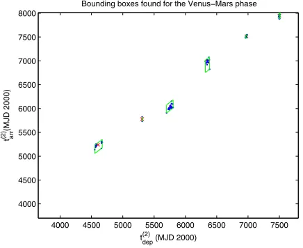
Figures 5 and 6 show the projected bounding boxes for each phase. These diagrams illustrate how an individual box in the first phase can be related to an individual box in the second phase to form a solution family. Nine solution families can be identified.

To perform the pruning for each phase, 120 random points were generated in phase 1 as described in section V (N1=

120), and the local optimizer was started from each point. Similarly, 350 random initial points were generated in phase 2 (N2= 350, 50 points per feasiblet

(2)

depinterval, with seven

initial feasible intervalsI1, . . . ,I6). Four local optimizations

from each initial feasible point in phase 2 were performed (N3 = 4), to evaluate feasibility with respect to the gravity

assist manoeuvre (Step 3 of Algorithm 2). After the gravity assist calculations and backward constraining, 220 feasible vectors were found in phase 1 (Q1= 220), while 65 vectors

were left in phase 2 (Q2 = 65). The mean shift clustering

algorithm was run with bandwidth value of 230 and 270 in phases 1 and 2, respectively. A total of 389,805 calls to the Lambert solver were required for the pruning phase (650 s CPU time)

Differential evolution with a population size of 20 indi-viduals and parameter values F = 0.8 and CR = 0.8 was employed to search for an optimal solution for each of the six solution families located. The algorithm was initially run for

N4= 200iterations for each solution family. This was done

to select the most promising solution family. Afterwards, Differential Evolution was run for N5 = 2000 iterations

for the selected solution family. A total of 192,000 Lambert solver calls were performed during the optimization phase (215 s CPU time). The returned result gave the following values for the decision variables: t0 = 4469.9, T_of(1) =

171.7855,T_of(2)= 682.4994,r(2)

= 0.5371,θ(2)

4000 4500 5000 5500 6000 6500 7000 7500 4000

4500 5000 5500 6000 6500 7000 7500 8000

Bounding boxes found for the Earth−Venus phase

t₀ (MJD 2000)

tarr

(1)

(MJD 2000)

Fig. 5. Illustration on the located bounding boxes on thet0−t(1)arrplane for

the estimates of the feasible regions for the Earth-Venus phase. dimensions

4000 4500 5000 5500 6000 6500 7000 7500 4000

4500 5000 5500 6000 6500 7000 7500 8000

Bounding boxes found for the Venus−Mars phase

t_dep(2) (MJD 2000)

tarr

(2)

(MJD 2000)

Fig. 6. Projection on thet(2)_dep−t(2)_arrplane of the located bounding boxes for the estimates of the feasible regions for the Venus-Mars phase. The actual bounding boxes are in six dimensions

rad, φ(2)

= −0.0073 rad, α(2)

= 0.5037. The resulting impulsive manoeuvres were:∆v(1)dep= 2.9743km/s,∆v

(1) ga =

8.547×10−5_km/s,

∆v(2)DSM= 0.4729km/s,∆v (2)

b = 2.0158

km/s, giving a total∆vvalue of 5.4630 km/s. Figure 7 shows the corresponding spacecraft trajectory projected on the plane defined by the Earth’s rotation.

Notice that the tolerance of the Lambert solver was relaxed at10−6for the pruning phase, and tightened at10−14for the Differential Evolution optimization phase. This was done in order to save computation time, as only an estimate of the feasible regions is found through the pruning method, and the regions found are not very sensitive to the tolerance value.

VIII. CONCLUSIONS

A method has been presented for the design of optimal multiple gravity assist trajectories with deep space manoeu-vres. A pruning method which considers the sequential nature

−3 −2 −1 0 1 2

x 108 −2

−1.5 −1 −0.5 0 0.5 1 1.5 2

x 108

x [km] Earth−Venus−Mars trajectory

y [km]

Mars orbit

Venus orbit

Venus swingby

departure

Earth orbit

Sun

Deep space manoeuvre braking manoeuvre

Fig. 7. Representation of the best trajectory found when Differential Evolution was applied to the pruned search space

of the problem has been described. The method locates feasi-ble vectors using local optimization and applies a clustering algorithm to find reduced bounding boxes which can be used in a subsequent optimization step. Since multiple local minima remain within the pruned search space, the use of a global optimization method, such as Differential Evolution, has been suggested for finding solutions which are likely to be close to the global optimum. Two case studies have been presented based involving missions with deep space manoeuvres.

ACKNOWLEDGMENT

This work has been funded by the European Space Agency under project Ariandna 06/4101.

REFERENCES

[1] J.T. Betts. Practical methods for optimal control using nonlinear programming. SIAM, Philadelphia, 2001.

[2] M. Vasile, L. Summerer, and P. De Pascale. Design of earth–mars transfer trajectories using evolutionary branching technique. Acta Astronautica, 56:705–720, 2005.

[3] D. Izzo, V. M. Becerra, D. R. Myatt, S. J. Nasuto, and J. M. Bishop. Search space pruning and global optimisation of multiple gravity assist spacecraft trajectories. Journal of Global Optimisation, 38:283–296, 2007.

[4] R.H. Battin. An introduction to the mathematics and methods of astrodynamics. AIAA, Reston, 1999.

[5] D.A. Vallado. Fundamentals of Astrodynamics and Applications. Kluwer Academic Publishers, London, 2001.

[6] W.E. Wiesel. Spacecraft Dynamics. Irwin McGraw-Hill, Boston, Mass., 1997.

[7] D. Comaniciu and P. Meer. Mean shfit: a robust approach toward feature space analysis. IEEE Transactions on Pattern Analysis and Machine Intelligence, 24:603–619, 2002.

[8] Z. Michalewicz and M. Schoenauer. Evolutionary algorithms for con-strained parameter optimization problems.Evolutionary Computation, 4(1):1–32, 1996.

[9] R. Storn and K. Price. Differential Evolution—a simple and efficient heuristic for global optimization over continuous spaces. Journal of Global Optimisation, 11:341–359, 1997.