Robust adaptive control for a hybrid solid oxide fuel cell system

Rochester Institute of Technology

RIT Scholar Works

Theses Thesis/Dissertation Collections

5-1-2011

Robust adaptive control for a hybrid solid oxide

fuel cell system

Steven Snyder

Follow this and additional works at:http://scholarworks.rit.edu/theses Recommended Citation

ROBUST ADAPTIVE CONTROL

FOR A HYBRID SOLID OXIDE

FUEL CELL SYSTEM

by

Steven Snyder

A Thesis Submitted in Partial Fulfillment of the Requirements for the Degree of Master of Science in Mechanical Engineering

Advised by

Dr. Tuhin Das, Assistant Professor, Mechanical Engineering Department of Mechanical Engineering

Kate Gleason College of Engineering Rochester Institute of Technology

Rochester, New York May 2011

Approved By:

Dr. Tuhin Das,

Assistant Professor, Mechanical Engineering Advisor

Dr. Agamemnon Crassidis,

Department Representative, Mechanical Engineering

Dr. Jason Kolodziej,

Thesis Release Permission Form

Rochester Institute of Technology

Kate Gleason College of Engineering

Robust Adaptive Control for a Hybrid Solid Oxide Fuel Cell System

I, Steven Snyder, hereby grant permission to the Wallace Memorial Library reproduce my thesis in whole or part.

Steven Snyder

Acknowledgments

In many ways, I consider myself fortunate for those I had the privilege to collaborate

with throughout my graduate work. I would like to acknowledge the invaluable

assis-tance of my advisor, Dr. Tuhin Das. I am wholeheartedly thankful for his guidance,

which helped me learn; his support, which helped me grow; and his encouragement,

which helped me stay motivated. I would also like to thank my labmates, W. John

Nowak and Sophia Su, for making the lab more than a place for work.

This work was supported in part by the Office of Naval Research under grant

Abstract

Solid oxide fuel cells (SOFCs) are electrochemical energy conversion devices. They

offer a number of advantages beyond those of most other fuel cells due to their high

operating temperature (800-1000℃), such as internal reforming, heat as a byproduct,

and faster reaction kinetics without precious metal catalysts. Mitigating fuel

starva-tion and improving load-following capabilities of SOFC systems are conflicting control

objectives. However, this can be resolved by the hybridization of the system with an

energy storage device, such as an ultra-capacitor. In this thesis, a steady-state

prop-erty of the SOFC is combined with an input-shaping method in order to address the

issue of fuel starvation. Simultaneously, an overall adaptive system control strategy

is employed to manage the energy sharing between the elements as well as to

main-tain the state-of-charge of the energy storage device. The adaptive control method is

robust to errors in the fuel cell’s fuel supply system and guarantees that the fuel cell

current and ultra-capacitor state-of-charge approach their target values and remain

uniformly, ultimately bounded about these target values. Parameter saturation is

employed to guarantee boundedness of the parameters. The controller is validated

Contents

Acknowledgments . . . . iv

Abstract . . . . v

List of Figures . . . . viii

Nomenclature. . . . x

1 Introduction . . . . 1

1.1 Motivation . . . 1

1.2 Basics of SOFCs . . . 2

1.3 Literature Review . . . 4

2 Fuel Cell System . . . . 9

2.1 System Description . . . 9

2.2 Fuel Utilization . . . 11

2.3 Open Loop Utilization Control . . . 14

2.4 Current Regulation . . . 16

2.5 Lag Induced by the Fuel Path . . . 18

2.6 Fuel Supply System . . . 19

2.7 Hybrid System . . . 22

3 Control Design . . . . 25

3.1 Control Objectives . . . 25

3.2 Adaptive Control . . . 25

4 Observations . . . . 36

4.1 Convergence of Ef c . . . 36

4.2 Parameter Convergence . . . 38

4.3 Reversal of c1 and c2 . . . 40

5 Experimental Results . . . . 42

5.2 Adaptive Control . . . 44

5.3 Effect of Adaptation . . . 50

6 Conclusion . . . . 55

List of Figures

1.1 SOFC Functional Schematic [1] . . . 3

2.1 Schematic Diagram of SOFC System . . . 9

2.2 Efficiency as a Function of Utilization in a Tubular SOFC . . . 12

2.3 Efficiency as a Function of Utilization in a Planar SOFC . . . 13

2.4 Open Loop SOFC Response to Current Draw . . . 13

2.5 Open Loop Control Of U . . . 15

2.6 Transient Control ofU through Current Regulation . . . 17

2.7 Effect of Current Regulation During Transience with First Order Dy-namics . . . 17

2.8 Effect of Current Regulation During Transience with Rate Limit Dy-namics . . . 17

2.9 Delays Along the Fuel Path and Sensor Placement . . . 18

2.10 Schematic of Hybrid System . . . 23

3.1 Adaptive Control Approach . . . 26

4.1 Simulation Results Suggesting Parameter Convergence . . . 39

5.1 Experimental Hardware-in-the-Loop Test Stand Setup . . . 43

5.2 Adaptive Control under Step Changes iniL . . . 45

5.3 Adaptive Control Efficiency Estimates . . . 46

5.4 Adaptive Control Saturation in ¯η2 . . . 47

5.5 Adaptive Control with 15% offset FSS . . . 49

5.6 Controller Performance Comparison with Zero and Non-zero Steady-state FSS Tracking Error . . . 50

5.7 Comparison ofU Between a Controller with Adaptation and One With-out . . . 51

Nomenclature

F Faraday’s constant = 96485.34 [coulomb/mol]

k Anode recirculation fraction

N Number of moles [moles]

Ncell Number of cells in series

˙

Nair Molar flow rate of air [moles/sec]

˙

Nf Molar flow rate of fuel [moles/sec]

˙

Nf,d Molar flow rate demand of fuel [moles/sec]

˙

Nin Anode inlet flow rate [moles/sec]

˙

No Anode exit flow rate [moles/sec]

n Number of electrons participating in electrochemical reaction [= 2]

R Species rate of formation [moles/sec]

Ru Universal Gas Constant 8.314 [J/mol/K]

T Temperature [K]

V Volume [m3]

X Mole fraction

Vcell Cell voltage [V]

U Fuel utilization [%]

Uss Steady state fuel utilization [%]

Vf c Fuel cell voltage [V]

if c Fuel cell current [A]

VL Load current [V]

iL Load current [A]

Vuc Ultra-capacitor voltage [V]

iuc Ultra capacitor current [A]

η1 Unidirectional dc/dc converter efficiency

η2 Ultra-capacitor grid bi-directional dc/dc converter efficiency

β1 1/η1

β2 1/η2

β12 η1/η2

C Capacitance value 250 [F]

Es Error in ultra-capacitor state of charge

Ef c,t Error between if c,t−if c,d

Ef c,t Error between if c−if c,t

Ef l Error between ˙Nf −N˙f,d

SOC State of charge

S State of charge of the ultra-capacitor

St Target state of charge of the ultra-capacitor

if c,t Fuel cell current target [A]

if c,d Fuel cell current demand [A]

DC Direct current

¯

η1 Estimated unidirectional DC/DC converter efficiency

¯

η2 Estimated ultra-capacitor grid bi-directional DC/DC converter efficiency

¯

β1 1/η¯1 ¯

β2 1/η¯2 ¯

β12 Estimated ratio of η1/η2

ei Error between βi−β¯i wherei is 1, 2, or 12

γi Adaptation gain for ¯ηi wherei is 1, 2, or 12

Subscripts

a Anode control volume

c Cathode control volume

Chapter 1

Introduction

1.1

Motivation

Rising energy demands and increased environmental awareness are straining our fossil

fuel-based energy infrastructure, causing prices to climb. Because of this, alternative

energy sources have become an important, and very attractive, area of research [2].

One such energy technology is the fuel cell. It has a number of advantages, such

as efficiency, simplicity, and low green house emissions [1]. Many fuel cell

technolo-gies have been developed over the past few decades, such as Polymer Electrolyte

Membrance Fuel Cells (PEMFC), Alkaline Fuel Cells (AFC), Solid Oxide Fuel Cells

(SOFC), and Molten Carbonate Fuel Cells (MCFC) [3].

One particular type of fuel cell showing significant potential is the SOFC [1]. The

three main components to a fuel cell are the electrolyte, anode, and cathode. SOFCs

use zirconia doped with 8-10 mole % yttria as the electrolyte. This is a solid state

material with a high capability of conducting oxygen ions. The anode is typically

a zirconia cermet, a mixture of a ceramic and metal. The cathode is composed of

strontium-doped lanthanum manganese [1]. Mass transport of reactant and product

gases must be allowed by the anode and cathode.

SOFCs operate at high temperatures (800-1000℃). This gives them advantages

beyond those shared with most other fuel cells, such as internal reforming (and

in a bottoming cycle), and faster reaction kinetics without precious metal (platinum)

catalysts [1, 3, 4]. Moreover, the high operating temperatures provide the capability

for combined heat and power (CHP) systems by using a gas turbine (GT) as a

bot-toming cycle to form a SOFC-GT hybrid system. Such a hybrid system can achieve

system efficiencies greater than the normal limitations of GT systems [5]. However,

due to their high cost and demanding safety requirements, the adoption of SOFCs

has not been extensive. Most installations occur in niche applications and are heavily

subsidized [6].

Like many other fuel cell technologies, SOFCs have a limited load following

capa-bility. This is because power transients result in fluctuations in the fuel utilization.

Fuel utilization is defined as the ratio of hydrogen consumption by the fuel cell to the

net available hydrogen in the anode inlet flow. A high utilization is needed for better

efficiencies. Typically, the desired utilization is around 80 to 90% [7, 8, 9]. However,

if the utilization is too high, the partial pressure of hydrogen in the fuel cell anode

can reduce, causing a voltage drop and irreversible damage due to anode oxidation.

This will be discussed in more detail in Chapter 2. So far, SOFC systems have been

limited to uniform power applications due to this deficiency. However, recently, there

has been an increasing interest in using SOFCs in mobile applications, where

respon-siveness is of paramount importance. In this regard, there is an intent to hybridize

the fuel cell in order to circumvent one of its largest drawbacks and make use of its

many advantages [10, 11], thereby making SOFCs competitive with PEM fuel cells,

which have traditionally been considered for hybrid vehicle applications.

1.2

Basics of SOFCs

The Solid Oxide Fuel Cell produces electricity through electrochemical reactions. The

oxygen, typically from air, flows into the cathode. The electrolyte is a ceramic

mate-rial that conducts only oxygen ions. The oxygen ions travel through the electrolyte

to the anode where they mix with hydrogen to produce water, in the form of steam,

and electrons. The electrons travel through the load and return to the cathode to

ionize more oxygen. Unlike other fuel cells, the electrolyte is not a membrane that

is permeable to molecules or atoms. It is strictly an ionic conductor, though only at

high temperatures [12]. Hence the high operating temperatures of SOFCs.

Figure 1.1: SOFC Functional Schematic [1]

While hydrogen acts as the primary fuel for producing electricity in SOFCs, it

can accept other fuels as well. Because of the high operating temperatures (800 to

1000℃) and the presence of catalysts, hydrogen can be generated through internal

reforming of hydrocarbon fuels within the anode chamber [1, 3]. Hydrogen can also be

generated through external reforming upstream of the fuel cell stack. Some of these

reforming reactions are endothermic, and, as such, require the recirculation of hot

reforming processes, such as POX (Partial OXidation) reforming, exist. In POX

reforming, fuel is partially oxidized in order to self-sustain the reforming process.

The mathematical formulation of fuel utilization, the ratio of hydrogen

consump-tion to the net available hydrogen in the anode of the SOFC, accounts for the

avail-able hydrogen, as well as the hydrogen that can be generated by means of internal

reforming [7, 9]. Because of the SOFC’s impurity tolerance, the reformer exhaust

gas mixture can be sent directly to the anode with little to no purification. Though

high utilization is required for high efficiency, if the utilization is too high, the partial

pressure of hydrogen in the anode can be reduced, leading to voltage drop and anode

oxidation, permanently damaging the fuel cell [14]. Typical target values for fuel

utilization are 80-90% [7, 8, 9].

1.3

Literature Review

There are many different types of fuel cells that have been researched in the past

few decades, each with its own advantages and disadvantages. Alkaline Fuel Cells

(AFC) were the first fuel cells to be used in real life applications [15]. AFCs are

used in space vehicles. They have a very high efficiency, and they operate at low

temperatures, around 200℃. Some disadvantages of the AFC are their slow reaction

kinetics, resolved by the use of porous electrodes with platinum catalysts, and their

sensitivity to carbon dioxide [16]. The cost associated with the platinum catalyst

and the air filtration system to remove CO2 poses significant restriction on the use

of AFCs.

Conversely, Molten Carbonate Fuel Cells (MCFC) are not poisoned by carbon

dioxide [1], and are able to use it as fuel. MCFCs are classified as high-temperature

fuel cells, operating temperatures around 650℃and are thus able to internally reform

CO and CO2. According to [17], MCFCs can only reach an efficiency of about 45 to

Direct Methanol Fuel Cells (DMFC) are another well-known fuel cell. They use

methanol as the direct fuel [18]. The benefit of this is reduced fuel storage space

due to the high density of methanol. DMFC is a relatively new technology that will

require significant improvement before it can feasibly be used in a larger class of

applications. Currently, these cells have a very low efficiency [1].

The first modern fuel cell module to be used as a power generator was the

Phospho-ric Acid Fuel Cell (PAFC) [19]. With operating temperatures of 150-200℃, PAFCs are

considered medium temperature fuel cells with operating temperatures around 200℃.

They use a proton-conducting electrolyte and have been able to achieve efficiencies

of ≈ 80% in providing power and heat. However, if producing only electricity, their

efficiency does not exceed 50%. The use of PAFCs has declined due to economical

issues [1].

One of the most commonly known fuel cells is the Polymer Electrolyte Membrane

Fuel Cell (PEMFC), also known as Proton Exchange Membrance Fuel Cells. They are

used primarily in transport and non-stationary applications due to their high power

density and low volume and weight [2, 6, 20, 21]. However, PEMFCs are limited by

their sensitivity to impurities in the fuel source, particularly carbon monoxide, CO,

and therefore require pure hydrogen to be supplied [22].

Solid Oxide Fuel Cells are high temperature fuel cells, operating around

800-1000℃. This removes the need for precious metal catalysts, reducing costs

signifi-cantly. Also, the high operating temperature allows for internal reforming to occur,

making SOFCs not only tolerant of carbon monoxide, but able to use it as fuel. The

efficiency of SOFCs can be very high with proper utilization of fuel within the fuel

cell stack. However, very high utilization can cause permanent damage to the fuel

cell anode [8]. This makes controlling the utilization properly very important in order

to maintain high efficiency without causing system damage. Because of these many

advantages, many researchers are interested in developing methods to increase the

The largest difficulty in using SOFCs is their limited load following capability,

which has precluded them from applications involving rapid power variations [6].

This is a common drawback to most fuel cells. It is generally attributed to the slow

dynamic response of the fuel and air delivery systems, consisting of valves, pumps,

and reformers [14, 23, 24, 25]. This slow response becomes evident as hydrogen or

oxygen starvation, drastic voltage drop, and/or compressor surge and choke. These

phenomena adversely affect the cell’s durability through anode oxidation [14], and

cell potential reversal, resulting in catalyst corrosion [26].

Many authors have addressed this issue by augmenting the fuel cell with an

elec-trical storage device to create a hybrid energy system. The authors of [23] interfaced

the primary, fuel cell, and secondary, ultra-capacitor, energy sources using

bidirec-tional power electronic devices. They developed a current control strategy in order

to minimize the fuel cell’s voltage drop during sudden increases in the load. The

control strategy is based on observing the terminal voltage of the fuel cell by

control-ling the ultra-capacitor currents. Simulation results show gradual prevention in any

substantial drop in the fuel cell voltage as the load power increases.

In [24], current in the PEM fuel cell is rate limited in order to prevent hydrogen

starvation. The strategy is based on a DC link voltage regulation that maintains the

fuel cell in a steady-state condition. Once again, the fuel cell is treated as the primary

power source with an ultra-capacitor as an auxiliary storage device. Power is drawn

from the ultra-capacitor in such a way as to minimize mechanical stresses on the fuel

cell. The ultra-capacitor current draw is synchronized with the PEMFC fuel flow and

the current draw of the load.

A nonlinear reference governor approach is developed in [27] to address the

prob-lem of oxygen starvation in PEM fuel cells. Parameter uncertainties are addressed

using a novel approach based on sensitivity functions. Simulation results are provided

to demonstrate the controller effectiveness at incorporating robust control while

developed in [25] for a fuel cell ultra-capacitor system. This controller minimizes

oxygen starvation, bounds the ultra-capacitor’s state-of-charge (SOC), and prevents

compressor surge and choke while responding to power demands from the load. In

[28], a MPC-based approach is used to improve battery performance and avoid fuel

cell and battery degradation.

Other authors have proposed a wide array of controllers for hybrid fuel cell systems

without specifically addressing any of the constraints mentioned above. Rule-based

control strategies where the hybrid system switches between discrete operating modes

are developed in [29, 30, 31]. In [29], the authors model the fuel cell ultra-capacitor

hybrid vehicle power system and design a model-based controller focusing on starting

conditions and the reverse regeneration of energy during braking.

In [30], the authors focus on cars powered by fuel cells with both ultra-capacitors

and batteries on-board as well. They attempt to reduce hydrogen consumption while

maintaining the state-of-charge of the ultra-capacitor and battery at acceptable levels.

The ultra-capacitor protects the fuel cell from load transience and captures a large

amount of energy from braking. For long periods of braking, or for larger power spikes,

the battery is used instead. Thus the fuel consumption can be reduced significantly.

An online power management system is proposed for a hybrid fuel cell system in

[31]. A multi-layered controller is discussed. The first layer controls what operating

mode the system is in. The second layer employs a fuzzy logic algorithm to manage the

power balance between the fuel cell and the auxiliary power module. The third, and

final, layer consists of sub-controllers that set the operating point for each subsystem

to reach the optimum performance.

In [32], an adaptive control strategy is used to adjust the output current of the fuel

cell according to the state-of-charge of the secondary power source. A two-loop control

strategy is proposed in [33] for a fuel cell ultra-capacitor hybrid system. The inner

loop maintains the DC bus voltage and the outer loop regulates the fuel cell current.

concerned with the thermal dynamics in their controller design. In [34], a non-linear

sliding-mode control is developed for the power management of a fuel cell system

that has been hybridized with an ultra-capacitor and a battery. The ultra-capacitor

module is used as an auxiliary transient power source while the battery is used for

power peaks of a longer duration. The authors of [35] use local minimization of an

equivalent fuel consumption variable to obtain optimal power distribution.

A differential flatness ([36]) based control strategy is developed by the authors

of [37] for a fuel cell ultra-capacitor system. The fuel cell acts as the main power

source with the ultra-capacitor acting as the secondary source. Two ultra-capacitors

are used in this set up, a DC link capacitor and an output capacitor. The DC link

capacitor connects both the primary and secondary power sources to the grid, and

the output capacitor connects the load and the grid through power electronics. The

fuel cell output voltage is kept constant and its dynamics are controlled.

Many of the works previously mentioned pertain to PEMFCs. Few deal with

hybrid SOFC systems, and those that do take an approach focused on very specific

setups or conditions. The work presented within this thesis seeks to provide a more

holistic approach to handling power management in a SOFC ultra-capacitor hybrid

Chapter 2

Fuel Cell System

2.1

System Description

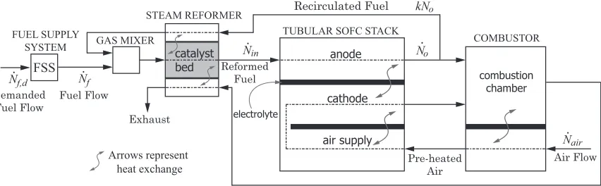
The system used in the ensuing analysis consists of a steam reformer, tubular SOFC,

and combustor. Methane is used as the fuel for the system; its molar flow rate is

denoted ˙Nf. Figure 2.1 contains a schematic of the overall fuel cell system. It should

be noted that the control strategy, and its analysis, developed in this thesis can be

extended to other system configurations and fuels.

catalyst bed

STEAM REFORMER

TUBULAR SOFC STACK

anode

cathode Nin

N_f

No

Nair

COMBUSTOR

combustion chamber

Reformed Fuel

Air Flow Exhaust

Fuel Flow

electrolyte

Pre-heated Air

Arrows represent heat exchange

air supply

kNo

Recirculated Fuel

GAS MIXER FUEL SUPPLY

SYSTEM

N_f,d Demanded

Fuel Flow

FSS

Figure 2.1: Schematic Diagram of SOFC System

The incoming fuel flow is combined with recirculated flow from the anode exhaust

in the gas mixer. The product of the mixer then flows through a catalyst (nickel

hydrogen-rich gas. The reactions are summarized in Equation (2.1).

CH4+H2O ­ CO+ 3H2O

CO+H2O ­ CO2 +H2 (2.1)

CH4+ 2H2O ­ CO2 + 4H2

This gas is supplied to the fuel cell anode, while pre-heated air is supplied to the

fuel cell cathode. The air acts as the oxygen source, and the oxygen is ionized in

the cathode. The electrolyte then conducts these oxygen ions to the anode where it

reacts with the hydrogen gas to form steam (H2O) and electrons. These electrons

pass through the external circuitry as the fuel cell current and return to the cathode

to ionize oxygen molecules. These reactions are summarized in Equation (2.2). It

should be noted that methane reforming continues in the anode as well. Figure 2.1

shows the primary electrochemical reactions of the SOFC stack. 1

2O2+ 2e

− _{→ O}2−

H2+O2− → H2O+ 2e− (2.2)

A known fraction k of the anode exhaust is recirculated, as previously mentioned.

The remainder of the anode exhaust is combined with the cathode exhaust in the

combustor. The combustor serves as the method of preheating the cathode air supply.

The exhaust of the combustor is used to supply heat to sustain the endothermic

reactions of the steam reformer.

The product of the reformer is a hydrogen-rich gas. This gas is supplied to the fuel

cell anode, while pre-heated air is supplied to the fuel cell cathode. A known fraction

k of the anode outlet gas is recirculated to supply heat to sustain the endothermic

reactions of the steam reformer. It is then mixed with the incoming fuel flow in the

gas mixer. The remaining anode outlet gas is combined with the cathode outlet gas

in the combustion chamber. The combustor also serves as the method of preheating

the air supply. The combustor exhaust is recirculated to supply additional heat to

2.2

Fuel Utilization

A single performance parameter, fuel utilization, is usually used to quantify the

per-formance of fuel cells. Fuel utilization,U, is defined as the ratio of hydrogen

consump-tion to the net available hydrogen in the anode [7]. A low fuel utilizaconsump-tion represents

inefficient system operation as a lot of fuel is being wasted. However, if the fuel

utilization is too high, hydrogen starvation can occur, which is unfavorable for stack

integrity as it may result in voltage drop or anode oxidation [14]. In order to balance

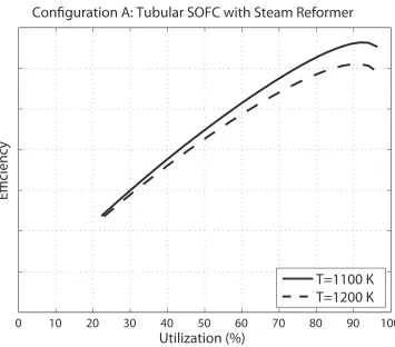
fuel efficiency and safe operation, target U values typically range between 80% and

90% [7, 8, 9]. Simulation results confirm this range for both tubular SOFCs, Figure

2.2, and planar SOFCs, Figure 2.3. Though the 80-90% range is sub-optimal, it

al-lows for high efficiency while maintaining a sufficient buffer to provide safe operating

conditions.

Fuel utilization can be expressed mathematically as

U = 1− N˙O(4XCH4,a+XCO,a+XH2,a)

˙

Nin(4XCH4,r+XCO,r +XH2,r)

(2.3)

[7, 9, 14], whereX represents the molar concentration in either the anode or reformer, as denoted by the subscripts a and r, respectively. ˙NO and ˙Nin are shown in Figure

2.1 and represent flow rates into and out of the anode.

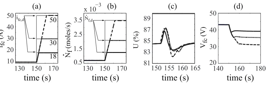
Figure 2.4 depicts the response of the fuel cell system to step changes in current.

In this simulation, Ncell = 50 and ˙Nf = 7 x 10−4moles/sec, which results in a steady

state utilization of Uss ≈85%. As can be seen in plot (b), the current drawn from the

fuel cell, if c, has a dramatic affect on the fuel utilization. Such drastic fluctuations in

U shorten the life of the fuel cell due to stack damage. In the next section, an

0 10 20 30 40 50 60 70 80 90 100

Utilization (%)

Efficiency

Configuration A: Tubular SOFC with Steam Reformer

T=1100 K

T=1200 K

0 10 20 30 40 50 60 70 80 90 100

Utilization (%)

Efficiency

Configuration B: Planar SOFC with POX Reformer

T=1100 K

T=1200 K

Figure 2.3: Efficiency as a Function of Utilization in a Planar SOFC

0

100

200

300

9

10

11

12

0

100

200

300

60

70

80

90

100

0

100

200 300

20

30

40

50

60

time (s)

time (s)

time (s)

i

fc

(A

)

U

(%)

V

fc

(V

)

10.5 11

(a)

(b)

(c)

2.3

Open Loop Utilization Control

Using the molar balance equations (Equation (2.4) and Equation (2.5)) and the rate

of electrochemical reaction equation (Equation (2.6)), the steady state utilization can

be found. In these equations, Nr and Na are the molar contents of the reformer and

anode, respectively,X represents the molar concentration of species, subscripts aand

r denote the anode and reformer, respectively, F = 96485.34Coul/mol is Faraday’s

constant,n= 2 is the number of electrons participating in an electrochemical reaction,

and if c is the fuel cell current.

d

dt(NrXCH4,r) = kN˙oXCH4,a−N˙inXCH4,r +RCH4,r+ ˙Nf

d

dt(NrXCO,r) = kN˙oXCO,a−N˙inXCO,r+RCO,r d

dt(NrXCO2,r) = kN˙oXCO2,a−N˙inXCO2,r− RCH4,r− RCO,r

d

dt(NrXH2,r) = kN˙oXH2,a−N˙inXH2,r −4RCH4,r − RCO,r

d

dt(NrXH2O,r) = kN˙oXH2O,a−N˙inXH2O,r + 2RCH4,r+RCO,r

(2.4)

d

dt(NaXCH4,a) = kN˙inXCH4,r−N˙oXCH4,a+RCH4,a

d

dt(NaXCO,a) = kN˙inXCO,r −N˙oXCO,a+RCO,a d

dt(NaXCO2,a) = kN˙inXCO2,r−N˙oXCO2,a− RCH4,a− RCO,a

d

dt(NaXH2,a) = kN˙inXH2,r−N˙oXH2,a−4RCH4,a− RCO,a−re

d

dt(NaXH2O,a) = kN˙inXH2O,r−N˙oXH2O,a+ 2RCH4,a+RCO,a+re

(2.5)

re =

if cNcell

nF (2.6)

Noting that the left hand side of Equation (2.4) and Equation (2.5) are zero at

steady state, the steady state utilization,

Uss=

1−k

(4nFN˙f/if cNcell)−k

(2.7)

can be found based on Equations (2.3) through (2.7). This relationship is independent

thus be called an invariant property of the fuel cell. In addition, since k,if c, and ˙Nf

are all known or measurable, Equation (2.7) can be used as an open-loop control law

to achieve a desired Uss by solving for the demanded fuel flow in terms of a given

current demand. This is summarized in Equation (2.8).

˙

Nf,d =

if c,dNcell

4nF Uss

[1−(1−Uss)k] (2.8)

While this control equation will achieve a steady-state behavior, let us examine its

effectiveness to transients in the current demand.

0 100 200 300 10

14 18 22

140 180 220 20 30 40 50

0 100 200 300 0.5

1 1.5x 10

−3 84 88 92 96 100

140 160 180

time (s) time (s) time (s)

ifc = ifc ,d (A ) U (%) Vfc (V ) 14 11

(a)

(b)

(c)

18 22

(d)

Figure 2.5: Open Loop Control Of U

Figure 2.5 shows results for multiple step changes in current demand. The system

is the same as in Figure 2.4. First order dynamics are assumed for the fuel supply

system with a time constant τ = 2sec and no steady-state offset. Notice that the

system remains operational for a 1A step change in current demand. This is a

sig-nificant improvement over the uncontrolled case. However, for larger step changes in

current demand, the utilization still rises too far, causing cell damage due to hydrogen

starvation and voltage drop. From the system response illustrated here, it is evident

2.4

Current Regulation

This section provides a brief summary of a previously developed feedback-based

strat-egy for minimizing fluctuations in fuel utilization. For more details and further

ex-planation, please refer to [38, 5]. While this work addresses fuel starvation, oxygen

starvation is not considered as it is seldom observed in typical SOFC systems. This

is because excess cathode air (air utilization ≈20 - 25 %, [39]), rather than coolants,

is used for temperature control [14]. Stack temperature control is important, but is

not considered in this work as stack temperature transients are considerably slower

(order of tens of minutes) compared to transient U (order of tens of seconds) [14, 40].

Hence, this is typically addressed in a decoupled manner by manipulating the cathode

air.

As seen in Figure 2.5, the actual fuel flow will not equal the demanded fuel flow

during transience due to the lag introduced along the fuel path. These delays will

be discussed in the following section. This inequality results in fluctuations in the

utilization. To attenuate these changes in utilization, Equation (2.8) can be reversed

to regulate the current draw based on the actual fuel flow, as seen in Equation (2.9).

if c=

4nF UssN˙f Ncell

1

[1−(1−Uss)k]

(2.9)

Figure 2.6 illustrates the current regulation approach. This approach assumes no

knowledge of the dynamic character of the FSS, though measurement of the actual

fuel flow, ˙Nf, is assumed available, and mitigates transient fluctuations in utilization

in a straightforward and effective manner, as seen in Figure 2.7.

From these results, it is evident that the transience in U has been significantly

reduced by the current regulation control approach. While the transience in U has

been diminished (see plot (c)), it has not be completely eliminated. Still, this control

strategy greatly increases the allowable current demand. One disadvantage to this

strategy is that it creates a discrepancy between the demanded fuel cell current, if c,d

Fuel supply system

(FSS)

Controller

Fuel cell stack and Power electronics

FUEL CELL SYSTEM

N

sensed N

i

Eq.(2.8)

Eq.(2.9)

i

(current drawn)

N

Reformer

Mass Flow Sensor data/command flow

Figure 2.6: Transient Control of U through Current Regulation

130 150 170 10

20 30 40 50

140 160 180

20 30 40 50

130 150 170 0.5

1.5 2.5 3.5

x 10−3

150 155 160 165 81

83 85 87 89

time (s)

time (s)

time (s)

time (s)

(a)

(b)

(c)

(d)

ifc (A ) U (%) Vfc (V ) Nf (m ol es /s

) Nf,d

i_fc,d

18 30 50

Figure 2.7: Effect of Current Regulation During Transience with First Order Dynam-ics

130 150 170 10

20 30 40 50

140 160 180

20 30 40 50

130 150 170 0.5

1.5 2.5 3.5

x 10−3

150 155 160 165 81

83 85 87 89

time (s)

time (s)

time (s)

time (s)

(a)

(b)

(c)

(d)

ifc (A ) U (%) Vfc (V ) Nf (m ol es /s

) Nf,d

i_fc,d

18 30 50

can be addressed by hybridizing the fuel cell with an energy storage device, such as an

ultra-capacitor. The addition of the energy storage device requires the maintenance of

the device’s state-of-charge (SOC) in order to prevent charge depletion or overcharge.

2.5

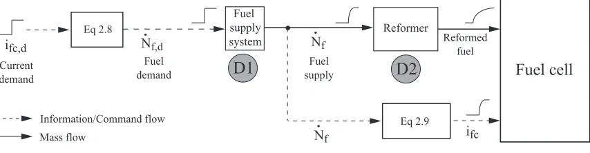
Lag Induced by the Fuel Path

As we saw previously, delays occurring along the fuel path cause disturbances to

the utilization during transients in fuel cell current demand. This lag is primarily

attributed to two sources, the fuel supply system, and the reformer, denoted D1

and D2, respectively, in Figure 2.9. The current regulation described in Section 2.4

Fuel supply system

Fuel cell

Nf,d

i_fc,d

Eq 2.8

ifc

Nf

Reformer

Reformed fuel Current

demand D1 D2

Fuel demand

Fuel supply

Information/Command flow

Mass flow

Eq 2.9

Nf

Figure 2.9: Delays Along the Fuel Path and Sensor Placement

compensates for D1. The remaining transience seen in Figure 2.7(c) and Figure 2.8(c)

are attributed to D2. While previous observations regarding the fuel supply system

have assumed a first order response or a ramped response, they apply to a wide range

of dynamic responses.

For perfect disturbance rejection,if c must be regulated to account for D2 as well.

Accomplishing this with a model-independent approach is a potential topic for future

research. Typically, the effect of D1 is more pronounced than D2. However, the effect

of D2 is magnified if the reformer’s void volume is much larger than the anode volume

or when there exist severe flow restrictions between the reformer and anode. Neither

2.6

Fuel Supply System

A model of the FSS is not required for control development of the hybrid system.

However, certain assumptions as to its character are made.

1. The FSS is assumed to be a combination of components such as a fuel pump

and/or valves and a controller. The closed-loop system delivers flow ˙Nf in

response to a demanded flow ˙Nf,d.

2. The state equation (or model) of the FSS is assumed to be unknown.

3. The delivered fuel ˙Nf is assumed to track the reference signal ˙Nf,d such that

|N˙f(t)| ≤β

³

|N˙f(t0)|, t−t0 ´

+γ

µ sup

t0≤τ≤t

|N˙f,d(τ)|

¶

(2.10)

where β is a class KL function and γ is a class K function. For definitions of these comparison functions see [41]. Equation (2.10) basically requires that ˙Nf

is eventually bounded by γ

³

sup_t0≤τ≤t|N˙f,d(τ)|

´

, where the magnitude of this

bound is dependent on the magnitude of ˙Nf,d.

The assumption that ˙Nf meets Equation (2.10) guarantees that ˙Nf will remain

bounded for all time, resulting in a stable FSS for bounded ˙Nf,d. Many common

system response fall into this category, including first order and ramped systems.

Thus, the assumption allows us to develop a controller that is applicable to a broad

class of FSS without knowing their specific structure.

Consider the first order system ˙

Nf

˙

Nf,d

(s) = c

τ s+ 1

where c and τ are positive constants. As a function of time, we see that

|N˙f(t)|=|N˙f(t0)e−

t−t₀

τ +cN˙_f,d(t)

³

1−e−t−τt0 ´

|.

Noting that e−(t−t0)/τ _{is strictly positive and less than 1, it is evident that}

|N˙f(t)| ≤ |N˙f(t0)|e−

t−t₀

τ +c sup

t0≤T ≤t

where|N˙f(t0)|e−(t−t0)/τ is a classKLfunctionβ ³

|N˙f(t0)|, t−t0 ´

, andcsup_{t0≤T ≤t}|N˙f,d(T)|

is a class K functionγ

³

sup_{t0≤T ≤t}|N˙f,d(T)|

´ .

Similarly, a ramped system with ˙Nf(t) = sgn( ˙Nf,d−N˙f)α(t−t0) + ˙Nf(t0), where

α > 0, can be shown to satisfy Equation (2.10), as well. If ˙Nf(t0) ≥ N˙f,d, the

system can be bounded by a first order response y(t) = (y(t0)−yd)e−λ(t−t0), where

λ ≤ α

yd−y(t0), y(t0) = ˙Nf(t0), and yd = ˙Nf,d, such that ˙Nf(t)≤ y(t) for all t. In this

case, the functions for β and γ given above for a first order system can be applied.

However, if ˙Nf(t0) < N˙f,d, then |N˙f(t)| < |N˙f,d| for all t. Therefore, the following

class KL functionβ and class Kfunction γ apply for all ramped FSS.

β =|N˙f(t0)|e−λ(t−t0),

γ = sup

t0≤T ≤t

|N˙f,d(T)|,

where a conservative λ can be calculated using extreme values of ˙Nf,d and ˙Nf(t0).

Any physical FSS will have a maximum and minimum flow rate, and ˙Nf,dis bounded.

Therefore, these extreme values will always exist.

Theorem 1. If N˙f satisfies Equation (2.10), then Ef l, defined as

Ef l ,N˙f −N˙f,d (2.11)

satisfies

|Ef l(t)| ≤βe(|Ef l(t0)|, t−t0) +γe

µ sup

t0≤τ≤t

|N˙f,d(τ)|

¶

(2.12)

where βe is a class KL function and γe is a class K function.

Proof. Using the triangle inequality [42] and Equation(2.11),

|Ef l(t)| ≤ |N˙f(t)|+|N˙f,d(t)|. (2.13)

Combining this result with Equation (2.12) results in

|Ef l(t)| ≤β

³

|N˙f(t0)|, t−t0 ´

+γ

µ sup

t0≤τ≤t

|N˙f,d(τ)|

¶

Rearranging Equation (2.11) and again applying the triangle inequality produces

˙

Nf(t0) =Ef l(t0) + ˙Nf,d(t0)⇒ |N˙f(t0)| ≤ |Ef l(t0)|+|N˙f,d(t0)|. (2.15)

As β is a class KL function, Equation (2.14) and Equation (2.15) can be combined to form

|Ef l(t)| ≤β

³

|Ef l(t0)|+|N˙f,d(t0)|, t−t0 ´

+γ

µ sup

t0≤τ≤t

|N˙f,d(τ)|

¶

+|N˙f,d(t)|. (2.16)

Next, note that

β

³

|Ef l(t0)|+|N˙f,d(t0)|, t−t0 ´ ≤     

β³2|Ef l(t0)|, t−t0 ´

if |Ef l(t0)| ≥ |N˙f,d(t−t0)|

β³2|N˙f,d(t0)|, t−t0 ´

if |Ef l(t0)| ≤ |N˙f,d(t−t0)|

Thus it follows that

β³|Ef l(t0)|+|N˙f,d(t0)|, t−t0 ´

≤ β³2|Ef l(t0)|, t−t0 ´

+β³2|N˙f,d(t0)|, t−t0 ´

.

Noting that a class KL function is decreasing with respect to the second term,

β

³

2|N˙f,d(t0)|, t−t0 ´

≤ β

³

2|N˙f,d(t0)|,0 ´

. Therefore, the flow error magnitude is

bounded as expressed in Equation (2.12) where

βe=β

³

2|Ef l(t0)|, t−t0 ´

is a class KL function and

γe

µ sup

t0≤τ≤t

|N˙f,d(τ)|

¶ =β

µ 2 sup

t0≤τ≤t

|N˙f,d(τ)|,0

¶ +γ

µ sup

t0≤τ≤t

|N˙f,d(τ)|

¶ + sup

t0≤τ≤t

|N˙f,d(τ)|

is a class K function.

Since Ef l satisfies Equation (2.12), it is ultimately bounded by some function of

|N˙f,d|. The developed control strategy for the hybrid system will be robust to this

Remark 1. Consider a system with input r and output y, where r, y ∈ Rn_{. If y(t)}

satisfies

||y(t)|| ≤β(||y(t0)||, t−t0) +γ µ

sup

t0≤τ≤t

||r(τ)||

¶

where β is a class KL function and γ is a class K function, then the error e(t) =

y(t)−r(t) satisfies

||e(t)|| ≤βe(||y(t0)||, t−t0) +γe

µ sup

t0≤τ≤t

||r(τ)||

¶

where βe is a class KL function and γe is a class K function, given by

βe(||e(t0)||, t−t0) = β(2||e(t0)||, t−t0)

γe

µ sup

t0≤τ≤t

||r(τ)||

¶ =β

µ 2 sup

t0≤τ≤t

||r(τ)||,0 ¶

+γ

µ sup

t0≤τ≤t

||r(τ)||

¶

+ sup

t0≤τ≤t

||r(τ)||

Proof. The proof is identical to that of Theorem 1.

2.7

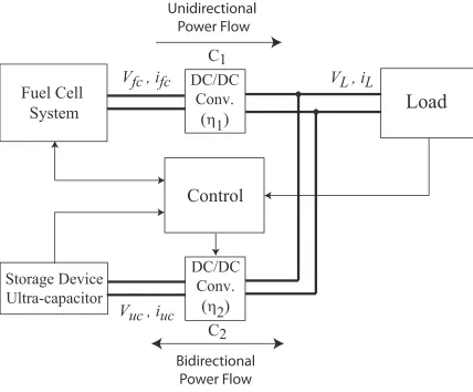
Hybrid System

Figure 2.10 depicts a schematic of the hybrid system. In it, the fuel cell and

ultra-capacitor are connected in parallel to the load via DC/DC converters, C1 and C2.

From this figure, it follows that the instantaneous power balance is

VLiL =η1Vf cif c+η2Vuciuc, (2.17)

whereη1 is the efficiency ofC1, andη2 is the efficiency ofC2. For control development

and analysis, the following are assumed:

• The load voltage, VL is held constant. This could be done by operating either

C1 orC2 in voltage control mode, and the other in current control mode. This

work uses C1 in voltage control mode andC2 in current control mode. Thus,C1

regulates the fuel cell voltage while C2 commands the ultra-capacitor current

DC/DC

Conv.

(

η

1

)

DC/DC

Conv.

(

η

2

)

Fuel Cell

System

Storage Device

Ultra-capacitor

Control

Load

V

fc

, i

fc

V

uc

, i

uc

V

L

, i

L

C

1

C

2

Unidirectional

Power Flow

Bidirectional

Power Flow

• The SOFC is operated in constant utilization mode, causing the fuel cell voltage

to vary with the power draw due to the voltage-current characteristics of the

fuel cell. This voltage is regulated by C1.

• The demanded fuel flow, ˙Nf,d, and the ultra-capacitor current,iuc, are treated as

the control inputs. It should be noted that iuc is commanded in both directions

as C2 is a bi-directional DC/DC converter.

• Measurements of Vf c,Vuc, iL, if c, and ˙Nf are available.

• The DC/DC converter efficiencies, η1 and η2 are unknown and time-varying,

but with known bounds

0≤η1,min≤η1(t)≤η1,max, 0≤η2,min ≤η2(t)≤η2,max.

Controller estimates for these efficiences are denoted ¯η1 ∈ [η1,min, η1,max] and

¯

Chapter 3

Control Design

3.1

Control Objectives

There are three primary control objectives for the hybrid system:

1. to minimize fluctuations in the fuel cell utilization

2. to maintain the SOC of the ultra-capacitor at a desired value, and

3. to meet load requirements while ensuring robustness to uncertainties in the

system.

3.2

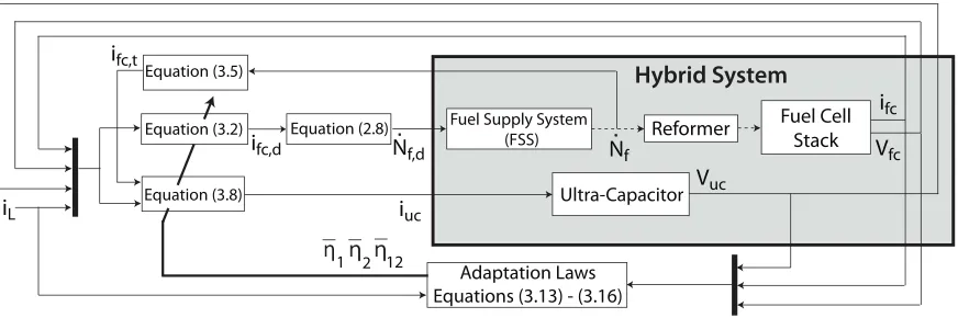
Adaptive Control

The schematic diagram shown in Figure 3.1 represents the adaptive controller for the

hybrid SOFC ultra-capacitor system. The fuel cell is the primary power source while

the ultra-capacitor acts as a secondary power source. The ultra-capacitor assists

dur-ing periods of power transience such that large fluctuations in the fuel cell utilization

are prevented. The efficiencies of the DC/DC converters that connect the power

sources to the load are unknown. The adaptive controller is designed to estimate

these values in suitable parametric form.

As shown in Equation (2.8), the demanded fuel flow, ˙Nf,d, is an algebraic function

Equation (3.5)

Equation (3.8)

Fuel Supply System (FSS)

Ultra-Capacitor

N_f,d

i_L

N_f

Hybrid System

i_fc

V_fc V_uc

i_fc,t

1 2 12

i_uc

Adaptation Laws Equations (3.13) - (3.16)

Reformer Fuel Cell Stack

Equation (3.2) Equation (2.8)

i_fc,d

Figure 3.1: Adaptive Control Approach

the demanded fuel cell current would ideally be calculated by Equation (3.1) in order

to meet the load requirements.

if c,d =

VLiL

η1Vf c

(3.1)

However, as the DC/DC converter efficiency is unknown, an estimate must be used

in place of the actual value. Also, during transience, the fuel cell will be incapable of

meeting the load demand due to the current shaping. The power deficit will be

com-pensated by the ultra-capacitor. This will result in a deviation of the ultra-capacitor

state of charge from the target value. The state of charge must be returned to its

target value based on the fuel cell current. Therefore, the demanded fuel cell current

can be practically calculated by Equation (3.2) in the presence of uncertainties.

if c,d =

VLiL

¯

η1Vf c

+g(Es) (3.2)

The function g(Es) is used to control the ultra-capacitor state of charge in order

to prevent overcharge or overdischarge. It is a function of Es, the error between

the measured state of charge, S, and the target state of charge, St, as expressed in

Equation (3.3).

Es =S−St (3.3)

as an energy buffer, as well as to allow it to absorb extra power during load

tran-sience. The state of charge is calculated by Equation (3.4), where the measured

ultra-capacitor voltage is Vuc, and the maximum ultra-capacitor voltage is Vmax.

S = Vuc

Vmax

(3.4)

Since ˙Nf is lagged by the FSS and the reformer, as discussed in Section 2.5, ˙Nf,d

(Equation (2.8)) is not realized. Instead, we assume the actual fuel flow is measured.

Based on the measured fuel flow, ˙Nf, the target fuel cell current,if c,tcan be expressed

as in Equation (3.5).

if c,t =

4nF UssN˙f Ncell

1

[1−(1−Uss)k]

(3.5)

However, we are not able to directly command if c,t due to the hardware setup.

Instead, we must calculate and command the ultra-capacitor current. Because of

delays in the fuel supply system, a discrepancy exists between the target fuel cell

current and the demanded fuel cell current, and consequently a power mismatch

occurs between the fuel cell and load. The difference between the target fuel cell

current and the demanded fuel cell current is known as Ef c,t, as shown in Equation

(3.6).

Ef c,t =if c,t−if c,d (3.6)

The ultra-capacitor must compensate for the power mismatch using Equation (3.7)

to control the ultra-capacitor current, iuc.

iuc= VLiL−η1Vf cif c,t

η2Vuc

(3.7)

Once again, the efficiencies of the power converters are unknown. Therefore,

esti-mates must be used in the actual implementation of Equation (3.7). Also, because

of uncertainties, the actual fuel cell current is not necessarily going to be match the

target current,if c 6=if c,t. Therefore, Equation (3.8) is used in place of Equation (3.7)

in the presence of uncertainties.

iuc=

VLiL−η¯1Vf cif c,t

¯

η2Vuc

The function h(Ef c) is used to account for the discrepancy between the actual,

mea-sured fuel cell current, if c, and the target fuel cell current, if c,t. It is based on the

error between these two values, as expressed in Equation (3.9).

Ef c=if c−if c,t (3.9)

Based on Equation (3.2) and Equation (3.8), the following parameters are

identi-fied

β1 = 1

η1

, β2 = 1

η2

, β12 =

η1

η2

, (3.10)

with parameter estimates given by

¯

β1 = 1 ¯

η1

, β¯2 = 1 ¯

η2

, β¯12 = ¯

η1 ¯

η2

, (3.11)

and parameter errors represented as

e1 =β1−β¯1, e2 =β2−β¯2, e12 =β12−β¯12. (3.12)

The following parameter adaptation law is proposed for the system:

˙¯

β1 = −

VLiLEs

CVmaxVuc

γ1+g1, γ1 >0

˙¯

β2 =

VLiLEf c

Vuc

γ2+g2, γ2 >0 (3.13)

˙¯

β12 = −

Vf cif cEf c

Vuc

γ12+g12, γ12 >0

whereγ1,γ2, andγ12are constant parameter adaptation gains. The termsg1,g2, and

g12 are designed to maintain the boundedness of the parameter estimates as follows:

g1 =         

−d1 if ¯β1 ≥β1,max and d1 >0

or ¯β1 ≤β1,min and d1 <0

0 otherwise

d1 = −γ1VLiLEs/(CVmaxVuc)

(3.14)

g2 =         

−d2 if ¯β2 ≥β2,max and d2 >0 or ¯β2 ≤β2,min and d2 <0

0 otherwise

d2 = γ2VLiLEf c/Vuc

g12 =     

   

−d12 if ¯β12 ≥β12,max and d12 >0 or ¯β12≤β12,min and d12<0

0 otherwise

d12 = −γ12Vf cif cEf c/Vuc.

(3.16)

Of the three objectives listed in Section 3.1, the first is handled by the current

shaping method presented in Section 2.4. The second and third can be summarized as

a need to stabilize the origin (Es, Ef c) = (0,0) in the presence of a time varying load,

iL, via the design ofif c,d and iuc, as expressed in Equation (3.2) and Equation (3.8),

respectively. Moreover, the dynamics of the fuel supply system result in a transient

error between if c,d and if c,t, as expressed in Equation (3.6); the dynamics of which

are characteristic of the fuel supply system and are considered to be unknown during

the controller design. Based on certain general stability properties of the fuel supply

system error variable, Ef l = ˙Nf −N˙f,d, stability of the overall hybrid system can be

ensured, as proved by the following theorems.

Theorem 2. If the origin of Efl is exponentially stable, then E¯= [EsEfc,t Efc]T = 0

is guaranteed to be an exponentially stable equilibrium by inputs ifc,d andiuc expressed

in Equation (3.2) and Equation (3.8), respectively, with g(Es) andh(Efc)as described

below in Equation (3.17) and Equation (3.18), respectively, and parameter adaptation

laws Equations (3.13,3.14,3.15,3.16).

g(Es) = −ksEs, ks >0 (3.17)

h(Ef c) =kpEf c+kdE˙f c, kp, kd>0 (3.18)

Proof. A Fuel Supply System with exponential tracking of the ˙Nf,d reference signal

implies that constantsγ,ζ,r0 >0 exist such that the inequality expressed in Equation

(3.19) holds true.

Based on Equation (2.8) and Equation (2.9), as well as the error definitions, Equation

(2.11) and Equation (3.6), Ef l can be described as an algebraic function of Ef c,t as

shown in Equation (3.20). Note that σ is a known constant.

Ef l =σEf c,t, σ =

Ncell[1−(1−Uss)k]

4nF Uss

(3.20)

From Equation (3.19) and Equation (3.20), it stands that exponential stability of the

origin of Ef c,t is true as well, as described in Equation (3.21).

|Ef c,t(t)| ≤ |Ef c,t(t0)|e−ζ(t−t0), ∀|Ef c,t(t0)|<

r0

σ (3.21)

Equation (3.21), in conjunction with Converse Lyapunov Theorems [41], guarantees

that there exists a positive definite and decrescent Lyapunov function, ¯VF SS, that

satisfies the inequalities of Equation (3.22), where α2 > α1 >0, andα3 >0.

α1Ef c,t2 ≤V¯F SS(Ef c,t)≤α2Ef c,t2 , V˙¯F SS ≤ −α3Ef c,t2 (3.22)

In order to analyze the overall hybrid system, a Lyapunov function candidate for the

system is proposed in Equation (3.23).

¯

V = 1 2

µ

η2

η1

E2

s +kdEf c2 +

e2 1

γ1 + e22

γ2 + e212

γ12 ¶

+ ¯VF SS (3.23)

As can be seen in Equation (3.24), this Lyapunov candidate is both positive definite

and decrescent.

min µ

α1, kd,

η2 η1 , 1 γ1 , 1 γ2 , 1 γ12 ¶_¡ ¯

E2_+e2

1+e22+e212 ¢

≤V¯(x, t) (3.24)

¯

V(x, t)≤max µ

α2, kd,

η2 η1 , 1 γ1 , 1 γ2 , 1 γ12 ¶_¡ ¯

E2_+e2

1+e22+e212 ¢

Differentiating the Lyapunov candidate along the state trajectories produces

Equa-tion (3.25). Note that η1 andη2 are not differentiated as they are treated as constant

parameters in the adaptive control. In actuality, they may be slowly varying.

˙¯

V = η2

η1

EsE˙s+kdEf cE˙f c+

e1e˙1

γ1

+ e2e˙2

γ2

+ e12e˙12

γ12

The ultra-capacitor dynamics can be simply modeled by Equation (3.26), where

C is the capacitance. This can be combined with Equation (3.3) to produce Equation

(3.27).

˙

Vuc = −iuc

C (3.26)

˙

Es = −iuc

CVmax

(3.27)

Solving Equation (3.1) for the ultra-capacitor current, Equation (3.27) can be

rewrit-ten as in Equation (3.28). ˙

Es=−

VLiL−η1Vf cif c

η2VucCVmax

(3.28)

Based on the definitions of Ef c and Ef c,t from Equation (3.9) and Equation (3.6),

respectively, the fuel cell current can be expressed as in Equation (3.29).

if c=Ef c+Ef c,t+if c,d (3.29)

Equation (3.30) contains the state of charge error dynamics in terms of the states,

derived from Equation (3.2), Equation (3.28), and Equation (3.29).

η2

η1 ˙

Es =

Vf c(Ef c+Ef c,t)

CVmaxVuc

− VLiLe1 CVmaxVuc

− ksEsVf c CVmaxVuc

(3.30)

The fuel cell current error dynamics can be described in terms of the states by

combining Equation (3.1) and Equation (3.8) with the designed function h(Ef c)

ex-pressed in Equation (3.18), as shown in Equation (3.31).

kdE˙f c =

VLiLe2−Vf cif ce12

Vuc

−αEf c, α=kp+

¯

η1Vf c

¯

η2Vuc

>0 (3.31)

Once again, it should be noted that the parameters are treated as constants within

the controller. Therefore, the parameter error derivatives are the opposite of the

derivative of the parameter estimates (see Equation (3.32)).

˙

e1 =−β˙¯1, e˙2 =−β˙¯2, ,e˙12 =−β˙¯12 (3.32)

Substituting Equation (3.30), Equation (3.31), and Equation (3.32) into the

(3.33), where ¯Qis defined in Equation (3.34).

˙¯

V ≤E¯T_{Q¯E −¯} e1g1

γ1

− e2g2 γ2

− e12g12 γ12 (3.33) ¯ Q=           

ksm −m₂ −m₂

−m

2 α 0

−m

2 0 α3

          

, m = Vf c

CVmaxVuc

>0 (3.34)

Here, it should be noted that ¯Q can be guaranteed to be positive definite by proper

selection of the design parameterskpandks. This is becauseCandVmaxare constants,

and Vf c, Vuc>0 are bounded based on the range of operating conditions. Also,eigi is

strictly non-negative, as defined in Equations (3.13,3.14,3.15,3.16). Therefore, using

the Rayleigh Ritz Inequality [41], ˙¯V can be shown to be negative semi-definite as seen

in Equation (3.35). From Theorem 8.4 of [41], Equation (3.36) follows.

˙¯

V ≤ −E¯TQ¯E ≤ −¯ inf(λ_Q¯)||E||¯ 2 (3.35)

¯

E →0 as t→ ∞ (3.36)

Next, we relax the conditions on the Ef l. This guarantees stability for a much

larger class of FSS. However, due to the limited knowledge of the fuel supply dynamics

in this case, the following theorem only guarantees boundedness for the state errors

and cannot guarantee convergence to zero.

Theorem 3. If ˙Nf meets the conditions of Equation (2.10), allowing the application

of Theorem 1, E = [Es Efc]T is uniformly ultimately bounded under the control given

in Figure 3.1 with ifc,d and iuc designed as in Equation (3.2) and Equation (3.8),

Proof. First we define a Lyapunov candidate function as

¯

V = 1 2

µ

η2

η1

E2

s +kdEf c2 +

e2 1

γ1 + e22

γ2 + e212

γ12 ¶

. (3.37)

Differentiating along the system trajectories, and substituting Equation (3.30) and

Equation (3.31), along with the parameter adaptation laws, Equations (3.13,3.14,3.15,3.16),

results in

˙¯

V ≤ −ET_{QE +mE}

sEf c,t−

e1g1

γ1

− e2g2 γ2

− e12g12 γ12

, (3.38)

where

Q= 

ksm −m₂ −m

2 α



_{, m=} Vf c

CVmaxVuc

>0. (3.39)

As stated previously, the product eigi is strictly non-negative. Therefore, applying

the Rayleigh Ritz Inequality and Equation (3.20), Equation (3.38) can be expressed

as follows:

˙¯

V ≤ −ET_{QE +mE} sEf c,t

≤ −inf(λmin,Q)||E||2+m||E|||Ef c,t|

≤ −inf(λmin,Q)(1−θ)||E||2+||E||(m|Ef c,t| −θinf(λmin,Q)||E||), 0< θ <1

≤ −inf(λmin,Q)(1−θ)||E||2 <0 ∀ ||E||>

m θinf(λmin,Q)

|Ef c,t|

≤ −inf(λmin,Q)(1−θ)||E||2 <0 ∀ ||E||>

mσ θinf(λmin,Q)

|Ef l| (3.40)

Now that we have proved the existence of a bound for the state vector, E, we attempt to determine a value for the bound. Let δmax be defined such that

˙¯

V ≤ −inf(λmin,Q)(1−θ)δmax2 <0 ∀ ||E||> δmax = sup

µ

mσ|Ef l|

θinf(λmin,Q)

¶

∀t≥t0 (3.41)

Next, noting that if c,t and if c,d are strictly non-negative, and using properties of

relationship between Ef c,t and Ef l in Equation (3.20) allows

|Ef c,t| ≤ σ[βe(|Ef c,t(t0)|,0) +γe(sup|if c,d|)]

≤ σ[βe(|if c,t(t0)|,0) +γe(sup|if c,d|)] (3.42)

≤ σ[βe(sup(if c,t),0) +γe(sup(if c,d))].

From Equation (3.5) and Equation (3.2),

sup(if c,t) =

4nF UssN˙f,max Ncell

1

[1−(1−Uss)k]

,

sup(if c,d) = ¯β1,max

VLiL,max

Vf c,min

+ksSt, (3.43)

where the limiting values can be determined from the practical range of operation of

various components in the system. Combining Equation (3.41) and Equation (3.43),

results in

δmax =

µ

σVf c,max

CVmaxVuc,minθinf(λmin,Q)

¶

[βe(sup(if c,t),0) +γe(sup(if c,d))], (3.44)

which along with Equation (3.43), shows the existence of a δmax for finite system

operating conditions. Now, it can be shown that the trajectories of E converge to the

region ||E||< δmax in finite time. Let