Computation of laminated composite plates using integrated radial basis function networks

Computation of Laminated Composite Plates using Integrated Radial Basis

Function Networks

N. Mai-Duy1 A. Khennane2 and T. Tran-Cong3

Abstract: This paper reports a meshless method, which is based on radial-basis-function networks (RBFNs), for the static analysis of moderately-thick lam-inated composite plates using the first-order shear defor-mation theory. Integrated RBFNs are employed to repre-sent the field variables, and the governing equations are discretized by means of point collocation. The use of in-tegration rather than conventional differentiation to con-struct the RBF approximations significantly stabilizes the solution and enhances the quality of approximation. The proposed method is verified through the solution of rec-tangular and non-recrec-tangular composite plates. Numeri-cal results obtained show that the method achieves a very high degree of accuracy and a fast convergence rate.

keyword: laminated composite plate, radial-basis-function network, meshless method.

1 Introduction

Principal discretization methods for solving partial dif-ferential equations (PDEs) include a finite-difference (FD), element (FE), boundary-element (BE), finite-volume (FV) and spectral method. Among them, the FEM is the most widely used method in computational engineering. To integrate a weak form and interpolate a solution variable, the FEM requires the division of the domain of interest into a number of small elements that are connected together by a fixed topology (i.e. mesh). This task is seen to be quite cumbersome especially for problems involving complex geometries, large degrees of deformation and free/moving surfaces. The idea of developing numerical methods without using a mesh for the solution of PDEs has received considerable attention from the scientific and engineering research

communi-1_{Computational Engineering and Science Research Centre, USQ,}

Toowoomba, QLD 4350 Australia,

2_{Computational Engineering and Science Research Centre, USQ,}

Toowoomba, QLD 4350 Australia,

3_{Computational Engineering and Science Research Centre, USQ,}

Toowoomba, QLD 4350 Australia.

ties in recent decades. As the name suggests, there will not be any connectivity requirements between interpola-tion points, leading to an easy process of numerical mod-elling. A comprehensive review of meshless methods can be found in, for example, [Atluri and Shen (2002);Liu (2003)].

102 Copyrightc 2004 Tech Science Press CMC, vol.1, no.1, pp.101-??, 2004

a smoothing operation and is more numerically stable.

In this paper, the meshless IRBFN-based method is fur-ther developed for the static analysis of moderately-thick laminated composite plates using the first-order shear de-formation theory. The obtained results are compared to existing results from different methods reported in the literature. Indeed, laminated fibre composite plates are extensively used in aeronautics and space indus-tries, and much research effort has been dedicated to im-prove the ability to predict the behaviour of these struc-tures. Closed form solutions based either on the first-or higher-first-order shear deffirst-ormation thefirst-ory (e.g. [Whit-ney and Pagano (1970);Bert and Chen (1978);Reddy and Chao (1981);Reddy (1984);Pandya and Kant (1988); Liu, Zhang, and Zhang (1994)]) as well as 3D elastic-ity solutions (e.g. [Srinivas and Rao (1970);Pagano and Hatfield (1972);Wang and Tarn (1994)]) are available to assess the accuracy of the numerical methods.

A brief review of the first-order shear deformation the-ory is given in Section 2. The governing equations in-volve a large number of derivative terms, some of which are mixed partial derivatives. The discretization of these equations using DRBFNs and IRBFNs is presented in section 3. In section 4, the IRBFN method is used to analyze composite plates with different geometries and boundary conditions. The obtained results show that the present method attains fast convergence rates and high degrees of accuracy. Section 5 gives some concluding remarks.

2 First-Order Shear Deformation Theory of Lami-nated Composite Plates

The first-order shear deformation theory (FSDT) of lam-inated composite plates is an extension of the Reissner-Mindlin theory for homogeneous isotropic thick plates. The governing differential equations are well known, and their derivation can be found in details in Reddy (2004). However, for the sake of consistency an outline of the main equations will be given below.

In FSDT, the displacement field is given as

u = u0+zψx, (1)

v = v0+zψy, (2)

w = w0, (3)

where (u0,v0,w0) are the displacements of a point

situ-ated in the middle plane, the xy plane, andψxandψyare

respectively the rotations of the transverse normal, i.e. in the z direction, with respect to the y and x axes.

In the present theory of thick plate without membrane action, u0 and v0 are discarded. As a result, the strain

displacement relationships are given as

εxx = −z∂ψx

∂x , (4)

εyy = −z∂ψy

∂y , (5)

γxy = z ∂ψx

∂y −

∂ψy ∂x

, (6)

γyz = ∂w

∂y −ψy, (7)

γxz = ∂w

∂x +ψx. (8)

The stresses in any given lamina k are expressed as

           σxx σyy τxy τyz τxz            =      

Q11 Q12 Q16 0 0

Q12 Q22 Q26 0 0

Q16 Q26 Q66 0 0

0 0 0 C44 C45

0 0 0 C45 C55

                 εxx εyy γxy γyz γxz            . (9) The previous expression can be rewritten as

   σxx σyy τxy    =  

Q11 Q12 Q16

Q21 Q22 Q26

Q16 Q26 Q66

     εxx εyy γxy    (10) and τyz τxz =

C44 C45

C45 C55

γyz γxz

, (11)

where the terms Qi j and Ci j represent the stiffness

given as

Q11 = Q11cos4θ+Q22sin4θ

+2(Q12+2Q66)sin2θcos2θ, (12)

Q12 = (Q11+Q22−4Q66)sin2θcos2θ

+Q12(cos4θ+sin4θ), (13) Q16 = (Q11−Q12−2Q66)sinθcos3θ

+(Q12−Q22+2Q66)sin3θcosθ, (14)

Q22 = Q11sin4θ+Q22cos4θ

+2(Q12+2Q66)sin2θcos2θ, (15)

Q26 = (Q11−Q12−2Q66)sin3θcosθ

+(Q12−Q22+2Q66)sinθcos3θ, (16)

Q66 = (Q11+Q12−2(Q12+Q66)sin2θcos2θ

+Q66(cos4θ+sin4θ), (17)

C44 = C44cos2θ+C55sin2θ, (18)

C45 = (C55−C44)cosθsinθ, (19)

C55 = C44sin2θ+C55cos2θ. (20)

The terms Qi j and Ci j represent the stiffness constants

of a unidirectional orthotropic ply in its principal axes. They are given as

Q11 =

E1

1−ν12ν21

, (21)

Q22 =

E2

1−ν12ν21

, (22)

Q12 =

ν12E2

1−ν12ν21,

(23)

Q66 = G12, (24)

C44 = G23, (25)

C55 = G13. (26)

The moments and shears are defined as acting per unit length. They are given as

Mxx =

Z h/2

−h/2

σxxzdz, (27)

Myy =

Z h/2

−h/2σyy

zdz, (28)

Mxy =

Z h/2

−h/2τxy

zdz, (29)

Qx =

Z h/2

−h/2τxzdz

, (30)

Qy =

Z h/2

−h/2τyz

dz, (31)

where h is the thickness of the laminate. Substituting for the stresses using equations (10) and (11), the moments and shear forces are rewritten as

   Mxx Myy Mxy    =  

D11 D12 D16

D12 D22 D26

D16 D26 D66

     εxx εyy γxy    (32) and Qy Qx =

A44 A45

A45 A55

γyz γxz

(33)

with

Di j =

1 3

n

∑

(h3_k−h3_k−1)(Qi j)(k) i,j=1,2,6, (34)

Ai j = κ

n

∑

(hk−hk−1)(Ci j)(k). (35)

whereκ=5/6 is a shear correction factor. Considering the equilibrium of an infinitesimal plate element leads to the following equations

∂Qx ∂x +

∂Qy

∂y +q(x,y) =0, (36)

∂Mxy ∂x +

∂Myy

∂y =Qy, (37)

∂Mxy ∂x +

∂Mxx

∂x =Qx. (38)

Substituting for Qx , Qy, Mxx, Myy and Mxy, the

equilib-rium equations become

A45 ∂2_w ∂x∂y−

∂ψy ∂x

+A55 ∂2_w ∂x2 +

∂ψx ∂x

+A44 ∂2_w ∂y2−

∂ψy ∂y

+A45 ∂2_w ∂x∂y+

∂ψx ∂y

+q(x,y) =0, (39)

D16 −

∂2ψx ∂x2

+D26 − ∂2_ψy ∂x∂y

+D66 ∂2ψx ∂x∂y−

∂2_ψy ∂x2

+

D12 −

∂2_ψx ∂x∂y

+D22 − ∂2_ψy

∂y2

+D26 ∂2_ψx

∂y2 − ∂2_ψy ∂x∂y

=A44 ∂w

∂y −ψy

+A45 ∂w

∂x +ψx

, (40)

D16 −

∂2ψx ∂x∂y

+D26 − ∂2_ψy

∂y2

+D66 ∂2ψx

∂y2 − ∂2_ψy ∂x∂y

+

D11 −

∂2_ψx ∂x2

+D12 − ∂2_ψy ∂y∂x

+D16 ∂2_ψx ∂y∂x−

∂2_ψy ∂x2

=A45 ∂w

∂y −ψy

+A55 ∂w

∂x +ψx

104 Copyrightc 2004 Tech Science Press CMC, vol.1, no.1, pp.101-??, 2004

For a cross-ply laminated composite plate (00,900), the equilibrium equations reduce to

A55 ∂2_w

∂x2 + ∂ψx

∂x

+A44 ∂2_w

∂y2 − ∂ψy

∂y

+q(x,y)

=0, (42)

D66 ∂2_ψx ∂x∂y−

∂2_ψy ∂x2

+D12 − ∂2_ψx ∂x∂y

+D22 − ∂2_ψy

∂y2

=A44 ∂w

∂y −ψy

, (43)

D66 ∂2ψx

∂y2 − ∂2_ψy ∂x∂y

+D11 − ∂2ψx

∂x2

+D12 − ∂2_ψy ∂y∂x

=A55 ∂w

∂x +ψx

. (44)

3 Radial Basis Function Networks

RBFNs allow a conversion of a function from low-dimensional space (e.g., 1D-3D) to high-low-dimensional space in which the function can be expressed as a linear combination of RBFs [Haykin (1999)]

fe(x)≈f(x) = m

∑

w(i)g(i)(x), (45)

where fe and f are the exact and approximate functions,

respectively; superscripts denote the elements of a set of neurons; x the input vector; m the number of RBFs;

{w(i)}m

i=1 the set of network weights to be found; and {g(i)(x)}m

i=1the set of RBFs.

3.1 Direct (DRBFN) approach

The RBFN (45) is utilized to represent the original func-tion fe; subsequently, its derivatives are computed by

dif-ferentiating (45), e.g. those with respect to x

∂fe(x) ∂x ≈

∂f(x)

∂x =

∂ ∑m

i=1w(i)g(i)(x)

∂x =

m

∑

w(i)h(i)(x), (46)

∂2_f e(x) ∂x2 ≈ ∂2_f(x)

∂x2 = ∂ ∑m

i=1w(i)h(i)(x)

∂x =

m

∑

w(i)h(i)(x), (47)

where h(i)(x) =∂g(i)(x)/∂x and h(i)(x) =∂h(i)(x)/∂x are new basis functions for the approximation of the first-and the second-order derivatives of the original function

fe, respectively.

3.2 Indirect (IRBFN) approach

RBFNs are used to represent the highest-order deriva-tives in the system under consideration, e.g., ∂2fe/∂x2 and∂2fe/∂y2. Lower-order derivatives and the function itself are then obtained by integrating those RBFNs, e.g. those with respect to x

∂2_f e(x) ∂x2 ≈

∂2_f(x) ∂x2 =

m

∑

w(i)_[x]g(i)(x), (48)

∂fe(x)

∂x ≈

∂f(x)

∂x =

m+q1

∑

w(i)_[x]H_[x](i)(x), (49)

fe(x) ≈ f[x](x) = m+q2

∑

w(i)_[x]H(i)_[x](x), (50)

where subscript[x]denotes the quantities resulting from the process of integration along the x direction; q1 the

number of new centres in a subnetwork that is employed to approximate a set of nodal integration “constants”, q2=2q1; and H_[x](i)=

R

g(i)dx and H(i)_[x] =R

H_[x](i)dx (i= 1,2,· · ·,m) new basis functions for the approximation of the first-order derivative and the original function fe,

re-spectively. For convenience of presentation, the new cen-tres and their associated known basis functions in subnet-works are also denoted by the notations w(i)and H(i)(x) (H(i)(x)), respectively, but with i>m.

There are two expressions, namely f[x](x)and f[y](x), to

represent the function f(x)(

w_[x] 6=

w_[y] ). At the col-location points, they are forced to be exactly the same, i.e., f[x](x) = f[y](x) = f(x)(these nodal function values

are unknowns to be found); at other points, the function f can be taken to be the average value of f[x](x)and f[y](x).

{x(k)}_k=p ₁={c(k)}m

k=1, with p=m, yields

f,xx = Gw[x], (51)

f,x = H[x]w[x], (52)

f = H[x]w[x], (53)

where G, H and H are the design matrices associated with the approximation of the second-order derivative, the first-order derivative and the function, respectively;

w_[x]is the set of network weights in the x direction to be found; f={f(x(k))}m

k=1; f,x ={∂f(x

(k)₎

∂x }mk=1; and f,xx=

{∂2f_∂x(x2(k))}m_k=1. For the purpose of computation, the two

matrices G and H are augmented using zero-submatrices so that they have the same size as the matrix H. By solv-ing (53) with the general linear least-squares technique, the set of network weights can be expressed in terms of the nodal function values, as

w[x]=H− 1

[x]f, (54)

where H−_[x]1is the Moore-Penrose pseudo-inverse; and the dimensions of w[x], H

−1

[x] and f are (m+q2)×1, (m+

q2)×m and m×1, respectively.

Substituting (54) into the system (51)-(53) yields

f,xx = GH

−1

[x]f, (55)

f,x = H[x]H− 1

[x]f, (56)

f = If, (57)

where I is the unit matrix. Cross derivatives∂f2(x)/∂x∂y can be straightforwardly computed using the design ma-trices associated with the first-order derivatives (56). Al-though the order of differentiation makes no difference theoretically, due to numerical error, it would be more accurate to take the average of the two equivalent repre-sentations,

∂2_f ∂x∂y =

1 2 ∂ ∂x ∂ f ∂y + ∂ ∂y ∂ f ∂x ,

f,xy= 1 2

H_[x]H−_[x]1

H_[y]H−_[y]1f

+

H_[y]H−_[y]1

H_[x]H−_[x]1f

. (58)

Expressions of f and its derivatives at an arbitrary point

x can be given by

f(x) =1 2

h

H(_[x]1)(x),· · ·,H_[x](m+1)(x),· · ·,H(m+q1+_[x] 1)(x), · · · ]H−_[x]1f

+1 2

h

H(_[y]1)(x),· · ·,H(m+_[y] 1)(x),· · ·,

H(m+q1+_[y] 1)(x),· · ·iH−_[y]1f

, (59)

∂f(x)

∂x =

h

H_[x](1)(x),· · ·,H_[x](m+1)(x),· · ·,0,· · ·iH−_[x]1f,

(60)

∂f(x)

∂y =

h

H_[y](1)(x),· · ·,H_[y](m+1)(x),· · ·,0,· · ·iH−_[y]1f,

(61)

∂2_f(x) ∂x2 =

h

g(1)(x),· · ·,0,· · ·,0,· · ·iH−_[x]1f, (62)

∂2_f(x) ∂y2 =

h

g(1)(x),· · ·,0,· · ·,0,· · ·iH−_[y]1f, (63)

∂2_f(x) ∂x∂y =

1 2

h

H_[x](1)(x),· · ·,H_[x](m+1)(x),· · ·,0,· · ·iH−_[x]1

H[y]H

−1 [y]f +1 2 h

H_[y](1)(x),· · ·,H_[y](m+1)(x),· · ·,0,· · ·i H−_[y]1

H[x]H

−1 [x]f

. (64)

The field variables w,ψx andψy in the governing equa-tions (42)–(44) are represented by RBFNs, using either (45)–(47) for the DRBFN approach or (60)–(64) for the IRBFN approach. The system of PDEs is then dis-cretized by means of point collocation. The RBFN so-lutions thus satisfy the governing equations pointwise, rather than in the average sense. Both approaches di-rectly lead to square equation systems. In the case of Dirichlet boundary conditions, i.e. w,ψx and ψy pre-scribed along the whole boundary, the dimensions of the system matrix are 3n×3n (n—the number of data points) for the DRBFN approach and 3nip×3nip(nip—the

num-ber of interior points) for the IRBFN approach. The IRBFN matrix is slightly smaller than the DRBFN ma-trix because the IRBFN formulation is written in terms of nodal variable values rather than network weights.

4 Numerical Results and Discussions

106 Copyrightc 2004 Tech Science Press CMC, vol.1, no.1, pp.101-??, 2004

study will employ these basis functions whose form is

g(i)(x) =

q

(x−c(i))T_(x−c(i)_{) +a}(i)2_{, (65)}

where c(i) and a(i) are the centre and width of the ith MQ basis function, respectively, and superscript T de-notes the transpose of a vector. In the present study, the width of the ith MQ-RBF, a(i), is simply chosen to be the minimum distance from the ith centre to its neighbours.

For all problems, the shear correction factor is taken to be 5/6, and the interlaminar shear stresses are computed through 3D elasticity equilibrium equations. Let n and t denote the normal and tangent to an arbitrary edge of the plate, respectively. Simply-supported and clamped edge conditions, which are considered herein, can be ex-pressed as follows

Simply supported:

w=0,ψt=0,Mn=0, (66)

Clamped:

w=0,ψt=0,ψn=0, (67)

where

Mn=n2xMx+2nxnyMxy+n2yMy, (68)

ψn=nxψx+nyψy, (69)

ψt=nxψy−nyψx, (70)

in which nxand nyare the direction cosines at a boundary

point.

4.1 Problem 1

Consider a simply-supported cross-ply laminate a×a (Figure 1) with four layers 0o/90o/90o/0ounder a sinu-soidally distributed transverse load

q=q0sin

πx

a

sin

πy

a

.

The material properties are chosen to be [Reddy (2004)] E1=25E2,ν12=0.25,

G12=G13=0.5E2,G23=0.2E2

A number of uniform densities, namely

{11×11,17×17,21×21,· · ·,41×41}, are em-ployed to study the convergence behaviour of the present method. The IRBFN results are compared with those obtained by the DRBFN method, the close form FSDT solutions [Reddy (2004)] and the 3D-elasticity

solutions [Reddy (1984)]. All results are presented in dimensionless forms according to the following relations

w→ 100E2h

3

q0a4

w, (71)

{σxx,σyy,τxy} → h 2

q0a2

{σxx,σyy,τxy}, (72)

{τyz,τxz} → h

q0a

{τyz,τxz}. (73)

Table 1 presents the results obtained by the DRBFN and IRBFN methods. When compared to the close form solu-tions using FSDT [Reddy (2004)], it can be clearly seen that the IRBFN method is far superior to the DRBFN method with respect to both accuracy and convergence. For the IRBFN method, the percentage errors are very small and they are consistently reduced with increasing density. It is remarkable that a high degree of accuracy is achieved even with a small number of collocation points. For example, at a density of only 21×21, the error of the maximum displacement is about 0.02%. For the DRBFN method, it can be noticed that although the computed val-ues of the field variables (i.e. w,ψx andψy) are in good agreement with the close form solutions, large errors ap-pear in the calculation of their derivatives (e.g.σxx). The DRBFN method is thus very sensitive to noise, and one needs to pay special attention to the process of chosing network parameters in order to achieve good accuracy. On the other hand, the use of integration to construct the RBF approximations significantly stabilizes the solution and enhances the quality of approximation.

4.2 Problem 2

The present method is further verified through the so-lution of a composite plate with a curved geometry. A clamped circular plate with radius R under a uniform load q is considered here. The set of material properties is chosen as follows

E1=5.6×106,E2=1.2×106,ν12=0.26,

G12=G13=G23=0.6×106

The laminate is unidirectional with fibers oriented at

θ = 0o with respect to the global coordinates. A wide range of the radius-to-thickness ratio, R/h =

{10,16.67,25,50,100}, is investigated.

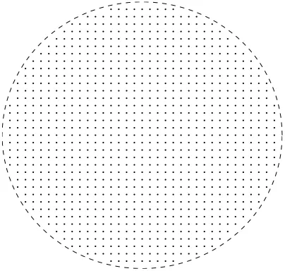
The present method does not require any underly-ing mesh. Nodes can thus be located in a flexible way. If one uses Cartesian-grid nodes to represent non-rectangular/irregular domains, the computational cost of generating data points can be significantly reduced. This discretization approach is generally recommended for use. For the present problem, the circular plate is first embedded in a square domain and the extended domain is then discretized using a Cartesian grid, i.e. an array of straight lines that run parallel to the x−and y−axes. The interior points are defined as grid points inside the analy-sis domain, while the boundary points are generated by the intersection of the grid lines with boundaries. Grid nodes outside the analysis domain are removed from the computations (Figure 3).

Convergence studies are conducted using 9 Cartesian grids, namely 11×11,17×17,· · ·,51×51. The cen-tral displacement of the plate is non-dimensionalized by a factor of D/qR4with D=3(D11+D22) +2(D12+2D66).

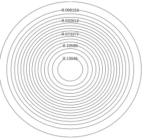
Table 4 lists the central displacement of the plate. The corresponding results obtained by FEM and the exact solution corresponding to the special case of thin plate [Wilt, Saleeb, and Chang (1990)] are also included for comparison. It is clearly indicated that the present method yields a very high order of accuracy. For ex-ample, at R/h=16.67, at least 4 decimal digits remain unchanged when densities are greater than 21×21. How-ever, when the thickness is reduced, higher densities are required to obtain a converged solution. This is proba-bly due to the fact that the thick-plate theories are used here. The results obtained are in good agreement with the FEM results, and they approach the thin-plate exact solution with decreasing thickness. The typical distribu-tion of the displacement obtained by the present method is displayed in Figure 4.

4.3 Problem 3

The results obtained in exampples 1 and 2 have clearly demonstrated the excellent accuracy achieved by the present method. It is believed therefore that the IRBFN method can now be confidently used to analyse non-trivial problems. Thus in this example, a plate similar in lamina lay-out to the one in Problem 1 with a cut-out square hole a/2×a/2 is analyzed under a uniform pres-sure q0. Good convergence is achieved, as shown in

Ta-ble 5, with a shear correction factor of 5/6 which is most suitable for isotropic plates.

Since close form or 3D elasticity solutions are not avail-able for this problem, the obtained results are compared to a FEM solution obtained with Abaqus [Hibbitt, Karls-son, and Sorenson (2006)]. Figure 5 shows discretiza-tions by the IRBFN and FEM. In the FEM solution, an eight-node conventional shell element with reduced in-tegration and six degrees of freedom per node is used. However, the commercial software ABAQUS does not reveal the value of the shear correction factor for com-posite plates, if any. Therefore it is not possible to make a quantitative comparison between the IRBFN and the ABAQUS results. Nonetheless, the similarity between the results is noticeable on the contour plots obtained with both methods as shown on Figures 6 and 7.

5 Concluding Remarks

108 Copyrightc 2004 Tech Science Press CMC, vol.1, no.1, pp.101-??, 2004

Acknowledgement: This research was supported by the Australian Research Council

References

Atluri, S. N.; Shen, S. P. (2002): The meshless local Petrov-Galerkin (MLPG) method. Tech. Science Press.

Bert, C.; Chen, T. (1978): Effect of shear deforma-tion on vibradeforma-tion of antisymmetric angle-ply laminated rectangular plates. International Journal of Solids and Structures 1978; 14:, vol. 14, pp. 465–473.

Haykin, S. (1999): Neural Networks: A Comprehen-sive Foundation. Prentice-Hall.

Hibbitt; Karlsson; Sorenson (2006): Abaqus (version 6.6-1). Hibbitt, Karlsson & Sorenson Inc., Pawtucket, RI, USA.

Kansa, E. (1990): Multiquadrics- A scattered data ap-proximation scheme with applications to computational fluid-dynamics-II. Solutions to parabolic, hyperbolic and elliptic partial differential equations. Computers and Mathematics with Applications, vol. 19, pp. 147–161.

Liu, G. (2003): Mesh Free Methods: Moving beyond the Finite Element Method. CRC Press.

Liu, P.; Zhang, Y.; Zhang, K. (1994): Bending So-lution of high order refined shear deformation theory for rectangular composite plates. International Journal of Solids and Structures, vol. 31, pp. 2491–2507.

Madych, W.; Nelson, S. (1988): Multivariate interpo-lation and conditionally positive definite functions. Ap-proximation Theory and its Applications, vol. 4, pp. 77– 89.

Madych, W.; Nelson, S. (1990): Multivariate inter-polation and conditionally positive definite functions, II. Mathematics of Computation, vol. 54, pp. 211–230.

Mai-Duy, N.; Tanner, R. (2005): Computing non-Newtonian fluid flow with radial basis function networks. International Journal for Numerical Methods in Fluids, vol. 48, pp. 1309–1336.

Mai-Duy, N.; Tran-Cong, T. (2001): Numerical so-lution of differential equations using multiquadric radial basis function networks. Neural Networks, vol. 14, pp. 185–199.

Mai-Duy, N.; Tran-Cong, T. (2003): Approximation of function and its derivatives using radial basis function networks. Applied Mathematical Modelling, vol. 27, pp. 197–220.

Mai-Duy, N.; Tran-Cong, T. (2005): An efficient indirect RBFN-based method for numerical solution of PDEs. Numerical Methods for Partial Differential Equa-tions, vol. 21, pp. 770–790.

Mai-Duy, N.; Tran-Cong, T. (2006): Solving bihar-monic problems with scattered-point discretisation us-ing indirect radial-basis-function networks. Engineerus-ing Analysis with Boundary Elements, vol. 30, pp. 77–87.

Pagano, N.; Hatfield, S. (1972): Elastic behaviour of multilayered bidirectional composites. AIAA Journal, vol. 10, pp. 931–933.

Pandya, B.; Kant, T. (1988): Flexural analysis of laminated composites using refined higher-order C0plate bending elements. Computer Methods in Applied Me-chanics and Engineering, vol. 66, pp. 173–198.

Park, J.; Sandberg, I. (1991): Universal approximation

using radial basis function networks. Neural Computa-tion, vol. 3, pp. 246–257.

Park, J.; Sandberg, I. (1993): Approximation and radial basis function networks. Neural Computation, vol. 5, pp. 305–316.

Reddy, J. (1984): A simple higher order theory of

lam-inated composite plates. Journal of Applied Mechanics, vol. 51, pp. 745–752.

Reddy, J. (2004): Mechanics of laminated composite plates and shells. Theory and analysis. CRC Press.

Reddy, J.; Chao, W. (1981): A comparison of closed-form and finite-element solutions of thick lami-nated anisotropic rectangular plates. Nuclear Engineer-ing and Design, vol. 64, pp. 153–167.

Srinivas, S.; Rao, A. (1970): Bending, vibration and buckling of simply supported thick orthotropic rectangu-lar plates and laminates. International Journal of Solids and Structures, vol. 6, pp. 1463–1481.

Wang, Y.; Tarn, J. (1994): A three-dimensional

Whitney, J.; Pagano, N. (1970): Shear deformation in heterogeneous anisotropic plates. Journal of Applied Mechanics 1970; 37:, vol. 37, pp. 1031–1036.

1

1

0

C

o

p

y

ri

g

h

t

c

2

0

0

4

T

ec

h

S

ci

en

ce

P

re

ss

C

M

C

,

v

o

l.

1

,

n

o

.1

,

p

p

.1

0

1

-?

?

,

2

0

0

4

Table 1 : Problem 1, a/h=10: Comparison of the accuracy of the DRBFN and IRBFN methods. It is noted that a(−b)means a×10−b.

Density DRBFN IRBFN

w(a/2,a/2) Error(%) σxx(a/2,a/2,h/2) Error(%) w(a/2,a/2) Error(%) σxx(a/2,a/2,h/2) Error(%)

11×11 6.8515(-1) 3.38 5.6738(-1) 13.72 6.6163(-1) 0.16 4.9759(-1) 0.26

17×17 6.8499(-1) 3.36 5.5818(-1) 11.88 6.6240(-1) 0.04 4.9852(-1) 0.07

21×21 6.8821(-1) 3.84 5.9050(-1) 18.36 6.6254(-1) 0.02 4.9868(-1) 0.04

27×27 6.8109(-1) 2.77 4.9086(-1) 1.61 6.6263(-1) 0.01 4.9878(-1) 0.02

31×31 6.7962(-1) 2.55 5.0164(-1) 0.54 6.6265(-1) 0.00 4.9881(-1) 0.01

37×37 6.7715(-1) 2.18 5.0036(-1) 0.29 6.6267(-1) 0.00 4.9884(-1) 0.01

41×41 6.7871(-1) 2.41 5.0226(-1) 0.67 6.6268(-1) 0.00 4.9885(-1) 0.01

Close form 6.627(-1) 4.989(-1) 6.627(-1) 4.989(-1)

u

ta

tio

n

o

f

L

am

in

at

ed

C

o

m

p

o

si

te

P

la

te

s

1

1

1

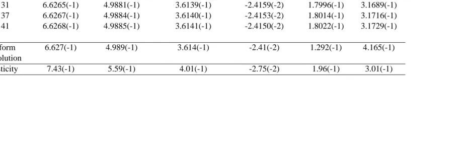
Table 2 : Problem 1: Displacement and stresses for a/h=10. It is noted that a(−b)means a×10−b.

Density w(a/2,a/2) σxx(a/2,a/2,h/2) σyy(a/2,a/2,h/4) τxy(a/2,a/2,h/2) τyz(a/2,0,0) τxz(0,a/2,0)

11×11 6.6163(-1) 4.9759(-1) 3.6084(-1) -2.4209(-2) 1.7678(-1) 3.1275(-1) 17×17 6.6240(-1) 4.9852(-1) 3.6125(-1) -2.4190(-2) 1.7877(-1) 3.1525(-1) 21×21 6.6254(-1) 4.9868(-1) 3.6133(-1) -2.4178(-2) 1.7933(-1) 3.1599(-1) 27×27 6.6263(-1) 4.9878(-1) 3.6137(-1) -2.4165(-2) 1.7978(-1) 3.1663(-1) 31×31 6.6265(-1) 4.9881(-1) 3.6139(-1) -2.4159(-2) 1.7996(-1) 3.1689(-1) 37×37 6.6267(-1) 4.9884(-1) 3.6140(-1) -2.4153(-2) 1.8014(-1) 3.1716(-1) 41×41 6.6268(-1) 4.9885(-1) 3.6141(-1) -2.4150(-2) 1.8022(-1) 3.1729(-1)

Close form 6.627(-1) 4.989(-1) 3.614(-1) -2.41(-2) 1.292(-1) 4.165(-1) FSDT solution

1

1

2

C

o

p

y

ri

g

h

t

c

2

0

0

4

T

ec

h

S

ci

en

ce

P

re

ss

C

M

C

,

v

o

l.

1

,

n

o

.1

,

p

p

.1

0

1

-?

?

,

2

0

0

4

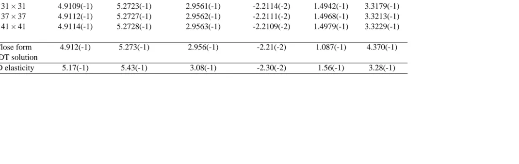
Table 3 : Problem 1: Displacement and stresses for a/h=20. It is noted that a(−b)means a×10−b.

Density w(a/2,a/2) σxx(a/2,a/2,h/2) σyy(a/2,a/2,h/4) τxy(a/2,a/2,h/2) τyz(a/2,0,0) τxz(0,a/2,0)

11×11 4.8911(-1) 5.2504(-1) 2.9481(-1) -2.2070(-2) 1.4400(-1) 3.2535(-1)

17×17 4.9066(-1) 5.2676(-1) 2.9542(-1) -2.2121(-2) 1.4750(-1) 3.2947(-1)

21×21 4.9091(-1) 5.2703(-1) 2.9553(-1) -2.2121(-2) 1.4844(-1) 3.3057(-1)

27×27 4.9105(-1) 5.2719(-1) 2.9559(-1) -2.2117(-2) 1.4915(-1) 3.3144(-1)

31×31 4.9109(-1) 5.2723(-1) 2.9561(-1) -2.2114(-2) 1.4942(-1) 3.3179(-1)

37×37 4.9112(-1) 5.2727(-1) 2.9562(-1) -2.2111(-2) 1.4968(-1) 3.3213(-1)

41×41 4.9114(-1) 5.2728(-1) 2.9563(-1) -2.2109(-2) 1.4979(-1) 3.3229(-1)

Close form 4.912(-1) 5.273(-1) 2.956(-1) -2.21(-2) 1.087(-1) 4.370(-1)

FSDT solution

u

ta

tio

n

o

f

L

am

in

at

ed

C

o

m

p

o

si

te

P

la

te

s

1

1

3

Table 4 : Problem 2: The central displacement of the plate. The grid densities are displayed in the case of the IRBFN method while the numbers of

elements are quoted in the case of FEM (Wilt, Saleeb, and Chang (1990) discretised a quarter of the circular plate with 12 and 48 elements which correspond to 48 and 192 elements displayed here for the full plate). It is noted that a(−b)and TPES mean a×10−band Thin Plate Exact Solution, respectively.

IRBFN FEM

R/h 11×11 17×17 21×21 27×27 31×31 37×37 41×41 47×47 51×51 48 192

10 1.3805(-1) 1.3851(-1) 1.3857(-1) 1.3859(-1) 1.3860(-1) 1.3860(-1) 1.3860(-1) 1.3860(-1) 1.3861(-1) 1.355(-1) 1.378(-1) 16.67 1.2879(-1) 1.2975(-1) 1.2988(-1) 1.2993(-1) 1.2995(-1) 1.2995(-1) 1.2996(-1) 1.2996(-1) 1.2996(-1) 1.266(-1) 1.291(-1) 25 1.2517(-1) 1.2683(-1) 1.2707(-1) 1.2716(-1) 1.2718(-1) 1.2720(-1) 1.2721(-1) 1.2721(-1) 1.2721(-1) 1.237(-1) 1.264(-1) 50 1.2044(-1) 1.2455(-1) 1.2514(-1) 1.2537(-1) 1.2545(-1) 1.2550(-1) 1.2552(-1) 1.2553(-1) 1.2554(-1) 1.211(-1) 1.247(-1) 100 1.1105(-1) 1.2251(-1) 1.2400(-1) 1.2463(-1) 1.2484(-1) 1.2498(-1) 1.2503(-1) 1.2507(-1) 1.2508(-1) 1.193(-1) 1.242(-1)

1

1

4

C

o

p

y

ri

g

h

t

c

2

0

0

4

T

ec

h

S

ci

en

ce

P

re

ss

C

M

C

,

v

o

l.

1

,

n

o

.1

,

p

p

.1

0

1

-?

?

,

2

0

0

4

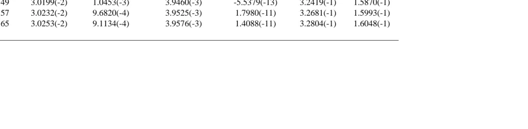
Table 5 : Problem 3: Displacement and stresses. It is noted that a(−b)means a×10−b.

Density w(a/2,a/8) σxx(a/2,a/8,h/2) σyy(a/2,a/8,h/2) τxy(a/2,a/8,h/2) τyz(a/2,0,0) τxz(0,a/2,0)

17×17 2.9590(-2) 8.0824(-4) 3.7160(-3) 1.6625(-8) -4.3448(-2) -4.0660(-2)

25×25 2.9900(-2) 1.3515(-3) 3.7761(-3) 1.5205(-9) 2.1391(-1) 1.0193(-1)

116 Copyrightc 2004 Tech Science Press CMC, vol.1, no.1, pp.101-??, 2004

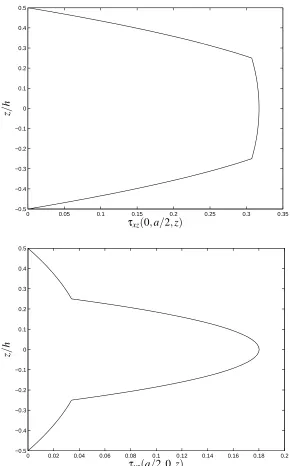
0 0.05 0.1 0.15 0.2 0.25 0.3 0.35

−0.5 −0.4 −0.3 −0.2 −0.1 0 0.1 0.2 0.3 0.4 0.5

τxz(0,a/2,z)

z

/

h

0 0.02 0.04 0.06 0.08 0.1 0.12 0.14 0.16 0.18 0.2

−0.5 −0.4 −0.3 −0.2 −0.1 0 0.1 0.2 0.3 0.4 0.5

τyz(a/2,0,z)

z

/

h

118 Copyrightc 2004 Tech Science Press CMC, vol.1, no.1, pp.101-??, 2004

0.13045 0.10599 0.073377 0.032612 0.008153

Figure 5 : Problem 3: Discretizations by IRBFN (left) and FEM (S8R elements) (right).

w

120 Copyrightc 2004 Tech Science Press CMC, vol.1, no.1, pp.101-??, 2004

a)σxx

b)σyy

c)τxy