A systems biology approach to explore the dynamics and interactions of the NF-κB signalling pathway

i

A Systems Biology Approach to Explore

the Dynamics and Interactions of the

NF-κB Signalling Pathway

Thesis submitted in accordance with the requirements of the University of Liverpool for the degree of Doctor in Philosophy by

James Boyd

ii Declaration

This thesis is the result of my own work, unless otherwise stated, and it is based upon the results from experimental and theoretical work performed as a PhD student between October 2009 and September 2012 in the department of Biological Sciences within the University of Liverpool.

Neither this thesis nor any part of it has been submitted in support of an application for another degree or qualification at this or any other university or institute of learning.

James Boyd

iii Abstract

The family of nuclear factor kappa B (NF-κB) transcription factors controls diverse mammalian signalling responses that mediate cell survival, inflammation, and immune response. Complex spatial and temporal dynamics observed in the NF-κB pathway are believed to determine gene expression profiles, which confer different physiological responses. The intricate and non-linear nature of the NF-κB system has benefited from the application of mathematical modelling methods which provide non-intuitive insights into the mechanism of cellular regulation.

It has become apparent that responses in signalling networks are influenced by complex spatial and temporal dynamics, which arise from a diverse range of competitive and combinatorial interactions. The systematic collection of quantitative data allows the application of a systems biology approaches to investigate and model complex biological systems. Through reiterative cycles of experimental and mathematical analysis it is possible to make predictions which generate testable hypotheses and guide future research.

iv Acknowledgements

I have had the pleasure of working with, or at least being in the rough proximity of people who have been working, so many fantastic people over the last three years that one page can hardly contain my gratitude. Firstly thank you to all my supervisors Prof Chris Sanderson, Dr Rachel Bearon (who first suggested this PhD to me, thank you!), Dr Violaine Sée, and, of course, Prof Mike White. I know I caused you all much worry over the last three years but thanks to your fantastic support I have now turned into a 'proper' scientist. I want to highlight the direct scientific contribution made by Dr John Ankers and Dr Antony Adamson whose work simply made this thesis possible. I also want to extend a special thanks to Dr Dave Spiller ('THE experimentalist') and Dr Pawel Paszek ('THE theoretician') who both mentored me throughout my PhD. It's probably not unfair to describe Dave as having been the carrot and Pawel the stick.

There are many other people in Liverpool and Manchester who have helped me over the years, both as friends and as scientists, that I wish to thank. I have to start with my fellow SABR students Karen and Simon who both made my PhD go way beyond the usual experience (ask anyone who knows us) and will no doubt appear in my nightmares for years to come. Then there is my long suffering fellow student Nick who helped keep me sane on those long summer nights together. I'd like to thank my fellow old man Baggers for helping me to put the world to rights, and for always being willing to let me show him how he's going wrong (in life as well as science). Thanks also go to Mark and Joe and all my other pub buddies for helping me to relax, to all the people at Warwick including Dan and Sascha the Dancing Queen, and to the many other members and ex-members of the White group Anne, Claire, Connie, David, Denise, Kate G, Kate S, Louise, Nisha, Raheela, Sheila, Steph, From the Liverpool office I want to thank Anne, Carol (who tried and failed to make me healthy), Cath, Damon (technically a traitorous Manchester student), Haleh (who made me hate white people), Marco, Sarah, and Stefan. It was a great environment to work in, with a seemingly never ending supply of tasty treats! There are also many other people whom I've had the pleasure of knowing throughout the last three years. You all know who you are and a big thank you to you all.

v Table of Contents

List of figures ... ix

List of Tables ... xi

List of Abbreviations ... xii

Chapter 1:

Introduction ... 1

1.1 Systems biology - a framework for modelling biological systems ... 2

1.2 Building a mathematical model of a biological system ... 3

1.3 Fluorescence microscopy – a tool for systems biology ... 6

1.3.1 Observing dynamic interactions beyond the diffraction limit ... 7

1.3.2 Fluorescence correlation spectroscopy ... 7

1.3.3 Raster image correlation spectroscopy ... 8

1.3.4 Förster resonance energy transfer and fluorescence lifetime imaging microscopy ... 10

1.4 The NF-κB signalling pathway – an exemplar to the systems biology approach ... 13

1.4.1 Overview ... 13

1.4.2 NF-κB as a biological oscillator ... 16

1.4.3 Mathematical modelling of NF-κB ... 18

1.4.3.1 Deterministic models of NF-κB ... 18

1.4.3.2 Population vs. single-cell approaches ... 19

1.4.3.3 Limitations of current models of NF-κB ... 20

1.5 Project aims ... 21

Chapter 2:

Materials and methods ... 22

2.1 Materials ... 23

2.1.1 Reagents ... 23

2.1.2 Expression vectors ... 23

2.2 Methods ... 23

2.2.1 Computational modelling and statistics ... 23

2.2.2 Sub-culturing cells ... 24

2.2.3 Transient transfection and imaging ... 24

vi

2.3.1 Live cell imaging ... 25

2.3.2 Dronpa Illumination Strategy ... 25

2.3.3 FCS and FCCS ... 25

2.3.4 RICS ... 26

Chapter 3:

Fitting a model of the NF-κB system using a

genetic algorithm approach ... 28

3.1 Introduction ... 29

3.1.1 Genetic algorithms ... 31

3.1.2 Sensitivity Analysis ... 33

3.2 Results ... 35

3.2.1 Improving the Ashall et al. model ... 35

3.2.2 Reconsideration of Ashall et al. data ...37

3.2.2.1 Peak detection ... 39

3.2.2.2 NF-κB single-cell pulsatile stimulation data ... 41

3.2.2.3 NF-κB under continuous TNFα treatment ... 43

3.2.3 Parameter search space and genetic algorithm development ... 46

3.2.3.1 Objective function and parameter scoring ... 46

3.2.3.2 Model conversion to number of molecules ... 48

3.2.3.3 Model scaling ... 54

3.2.3.4 Parameter search space ... 56

3.2.3.5 Exploring different genetic algorithm approaches ... 59

3.2.4 Model refit ... 63

3.2.4.1 Algorithm output parameter values ... 63

3.2.4.2 Introducing a delay in A20 activity ... 70

3.2.5 Global sensitivity using a genetic algorithm approach ...73

3.2.5.1 Parameter ordering outcome ...73

3.3 Discussion ... 76

Chapter 4:

Fluorescence

correlation

spectroscopy

optimisation and initial results ... 79

4.1 Introduction ... 80

4.2 Results ... 81

4.2.1 Initial setup ... 81

vii

4.2.2.1 Theoretical background... 86

4.2.2.2 Measuring Rhodamine 6G concentration ... 89

4.2.2.3 Single fluorophore detection ... 90

4.2.3 Measuring molecule diffusion and molecular mass ... 92

4.2.3.1 General experiment considerations and diffusion contribution . 92 4.2.3.2 EGFP monomer mobility in live-cells ... 96

4.2.3.3 Measuring molecular mass of fluorescently labelled p65 and IκBα in live cells ... 99

4.2.4 Measuring degree of binding between p65 and IκBα ... 103

4.2.5 General considerations ... 106

4.2.5.1 Photobleaching effects ... 106

4.2.5.2 Noise in data ... 107

4.2.5.3 Selection of number of components for diffusion model ... 108

4.3 Discussion ...111

Chapter 5:

Correlation spectroscopy studies applied to

the NF-κB signalling system ... 114

5.1 Introduction ... 115

5.2 Results ... 116

5.2.1 Observing the interaction of p65 with the cell-cycle related proteins E2F1 and E2F4 ... 116

5.2.2 Detecting intra-molecular p105 using FRET-FCS ... 121

5.2.3 Exploring the nuclear dynamics of p65 and IκBα ... 124

5.2.3.1 Detecting nuclear p65 and IκBα in non-stimulated cells ... 124

5.2.4 A RICS approach to map nuclear p65 and IκBα binding ... 127

5.2.4.1 RICS data analysis ... 127

5.2.4.2 Optimisation and imaging ... 128

5.2.5 Towards a diffusion based model of NF-κB ... 131

5.3 Discussion ... 144

Chapter 6:

General discussion... 147

6.1 General comment ... 148

6.1.1 Overall reflections ...148

6.1.2 Reflection on thesis aims ...148

viii

6.2.1 Summary of deterministic modelling of NF-κB ... 150

6.2.2 Comparing refitted and original parameter values ... 150

6.2.3 The collective effect of small parameter changes ... 152

6.2.4 Parameter sensitivities – the effect of A20 transcription ... 152

6.2.5 Delay in A20 activity ... 154

6.2.6 A specific prediction on the bindings rates of p65 and IκBα ... 155

6.2.7 Towards a diffusion based model of NF-kB. ... 156

6.3 Experimental work on NF-κB ... 157

6.3.1 The interaction between p65 and IκBα ... 157

6.3.2 Basal activity of p65 ... 158

6.3.3 Tethering of p65 ... 159

6.3.4 The interaction of p65 with cell cycle proteins E2F1 and E2F4 ... 160

6.4 Fluorescence fluctuation microscopy ... 161

6.4.1 As a tool for systems biology ... 161

6.5 Final comment ... 163

ix List of figures

Figure 1-1 Example of a protein interaction schematic. ... 4

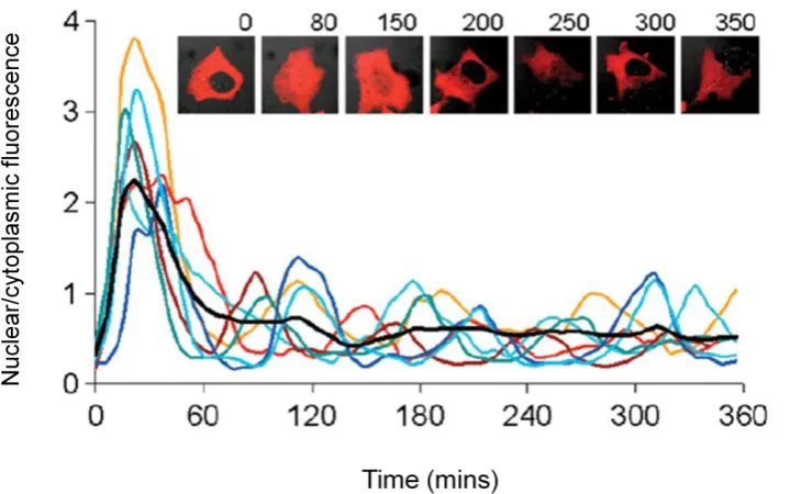
Figure 1-2 Complex protein dynamics observed using confocal microscopy. . 6

Figure 1-3 Schematic of FCCS experiment. ... 9

Figure 1-4 Principles of FRET. ... 12

Figure 1-5 The core NF-κB signalling system. ... 15

Figure 3-1 Schematic of a simple genetic algorithm. ... 32

Figure 3-2 Comparing molecule number and concentration of N:C ratio of NF-κB output by Ashall et al. model simulation. ... 36

Figure 3-3 Comparing NF-κB peak amplitudes using different normalisation methods. ... 38

Figure 3-4 Change in whole-cell p65-dsRedXP average fluorescence intensity per pixel. ... 39

Figure 3-5 Example of cell trace peak detection. ... 41

Figure 3-6 Analysis of P65-dsRedXP translocations in SK-N-AS cells pulsed with TNFα. ... 42

Figure 3-7 p65 oscillations following TNFα treatment. ... 45

Figure 3-8 Convergence of two types of genetic algorithm. ... 62

Figure 3-9 Simulated time course of parameter sets showing different characteristics. ... 65

Figure 3-10 Simulated time course of all conditions for new fit. ... 67

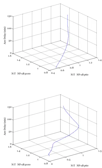
Figure 3-11 The effect of delay in A20 activity on pulse simulations. ... 71

Figure 3-12 Simulated time course of NF-κB with 100 min A20 activity delay. ... 72

Figure 4-1 Free diffusion of Rhodamine 6G in solution. ... 83

Figure 4-2 Measuring Rhodamine 6G concentration in solution. ...90

Figure 4-3 Single fluorophore detection in an Nrf2 expressing cell line. ... 91

Figure 4-4 Diffusion of EGFP monomer in live-cells. ... 98

Figure 4-5 Diffusion of p65 and IκBα in live-cells. ... 101

Figure 4-6 Estimated molecular mass of p65 and IκBα. ... 102

Figure 4-7 Detecting the interaction of p65 with IκBα. ... 104

Figure 4-8 Molecule number in confocal volume of p65 and IκBα. ... 105

x

Figure 4-10 Comparison of detector sensitivities at fast timescales between

GaAsp and APD detectors. ... 108

Figure 4-11 Comparing a three-component and one-component diffusion model fits. ... 110

Figure 5-1 FCCS study of p65 with E2F1 and E2F4. ... 118

Figure 5-2 Analysis of correlation curves for p65 and E2F1. ... 119

Figure 5-3 Analysis of correlation curves for p65 and E2F4. ... 120

Figure 5-4 Assessing the degree of bleed-through for the AmCyan fluorescent protein. ... 121

Figure 5-5 Confirmation of Dronpa photo-switching as observed using FCS. ... 122

Figure 5-6 Attempt to observe intra-molecular FRET-FCS using Dronpa photo-switching. ... 123

Figure 5-7 FCS and FCCS analysis of p65 and IκBα in BAC-BAC cells. ... 125

Figure 5-8 Comparing cytoplasmic and nuclear p65 and IκBα. ... 126

Figure 5-9 RICS background subtraction. ... 129

Figure 5-10 Mapping nuclear diffusion of p65 and IκBα . ... 130

xi List of Tables

xii List of Abbreviations

A20 Tumor necrosis factor, alpha-induced protein 3 BAC Bacterial Artifical Chromsome

cDNA Complementary deoxyribonucleic acid

CMV Cytomegalovirus

CPM Counts per molecule

DNA Deoxyribonucleic acid

DsRedXP DsRed-express, red fluorescent protein ECFP Enhanced green fluorescent protein EGFP Enhanced green fluorescent protein EMSA Electrophoretic mobility shift assay EYFP Enhanced yellow fluorescent protein

FBS Fetal Bovine Serum

FCS Fluorescence correlation spectroscopy FCCS Fluorescence cross-correlation spectroscopy FRAP Fluorescence recovery after photobleaching FRET Förster resonance energy transfer

GIGA Gene invariant genetic algorithm HeLa Human cervical carcinoma

IL-1 Interleukin-1

IκB Inhibitor of kappa B

IKK IκB Kinase

Kd Disassociation constant LHS Latin hypercube sampling

LMB Leptomycin B

LPS Lipopolysaccharide

LSM Laser scanning microscopy MEF Mouse embryonic fibroblast mRNA Messenger ribonucleic acid

NA Numerical aperture

xiii

Nrf2 Nuclear factor-E2-related factor 2

N:C Nuclear:Cytoplasmic cellular fluorescence ratio N:T Nuclear:Total cellular fluorescence ratio

ODE Ordinary differential equation PDE Partial differential equation

RHD Rel Homology Domain

RICS Raster image correlation spectroscopy ROI Region of interest

RRE Reaction rate equation

SD Standard deviation

1

2

1.1Systems biology - a framework for modelling biological systems

The application of a systematic approach to the study of scientific and social phenomena is an idea that has existed for many decades (Bertalanffy, 1972). A system can be defined as being an ensemble of interacting parts, the sum of which exhibits behaviour not localised in its constituent parts (Chen, 1993). The complex nature of biological phenomena have presented themselves as a natural case for the application of a systems biology approach, with the result that systems biology has been growing in popularity for the last 20 years (Chuang et al., 2010). Although it is also noted that there have historically been many studies that serve as what would now be called the systems biology approach (Hodgkin and Huxley, 1952; Noble, 2011; Turing, 1952).

The systems biology methodology of considering large interacting systems and the resulting complexity stands against the classical reductionist approach. This philosophy extends not only to the subject matter, but also to the whole approach of systems biology (Ideker et al., 2001). Systems biology relies on the systematic collection of data, and its systematic analysis. The cyclic and informative feedback between model analysis and experiment design, biological insight and new data, is crucial to the increased understanding of the complex systems studied.

3

system may be known, the nature of the interaction between components is often not, and modelling approaches provide a method of gaining a deeper understanding of the system. Moreover, a well-fitted mathematical model is able to produce specific, quantitative and testable hypotheses.

1.2 Building a mathematical model of a biological system

When building a mathematical model, the first focus should be towards what questions that are hoped to be addressed by the model. There is a hierarchy of spatial scales (“levels of biological organisation”) in biological systems, which ranges from genes, to proteins, to individual biological cells, to tissues, organs, and up to the individual organism that interacts with its environment (Southern et al., 2008). Consideration also needs to be given towards the temporal scale of biological processes, which ranges from microsecond for molecular interactions up to phenomena that occur over periods of years (Dada and Mendes, 2011).

4

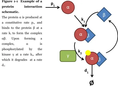
Figure 1-1 Example of a

protein interaction

schematic.

The protein α is produced at a constitutive rate p1, and

binds to the protein β at a rate k1 to form the complex

αβ. Upon forming a complex, α is phosphorylated by the kinase γ at a rate k2, after

which it degrades at a rate d1.

A tool often employed to represent biochemical reactions is the Law of Mass Action. This states the rate of the reaction is proportional to the concentration of the substrates (Murray, 2002). The law of mass action can be used in conjunction with the description framework to produce a system of reaction rate equations (RREs) (Bhalla, 2003). Figure 1-1 is an example of a protein-protein interaction schematic between two proteins. If the law of mass action is assumed true then the evolution of this system over time can be represented as a set of coupled ordinary differential equations (ODEs):

β

α

β

α

β

α

γ

Ø

p

k

d

5

(1-1)

(1-2)

- (1-3)

(1-4)

Here, the protein α is produced at a constitutive rate , and binds the protein at a rate to form the complex . Upon forming a complex, is phosphorylated by the kinase at a rate , after which it degrades at a rate

.

6

1.3 Fluorescence microscopy – a tool for systems biology

In 1994, it was discovered that green fluorescent protein (GFP) from the jellyfish Aequorea victoria could be fused with other proteins in many cell types to form fluorescent fusion proteins (Chalfie et al., 1994b). The subsequent onset of fluorescent fusion protein technology and development in time-lapse fluorescence microscopy has provided the ability to perform non-invasive measurement of protein spatiotemporal dynamics (Ankers et al., 2008; Spiller et al., 2010). An example of complex protein dynamics that can be observed using confocal microscopy is shown below.

7

1.3.1Observing dynamic interactions beyond the diffraction limit

Fluorescence microscopy represents a paradigm shift away from considering bulk cell behaviours, to considering the intracellular dynamics of proteins. It provides an excellent source for highly temporal data that can be ideal for informing mathematical models of biological systems. However, whilst population of protein behaviours can be observed using standard confocal microscopy, it does not have the power to resolve individual protein interactions. The well known Rayleigh limit for peak emission is given by (Born and Wolf, 1980),

(1-5)

where is the emission wavelength of the light emitted from the specimen being observed, and is the numerical aperture of the objective lens. For green light (wavelength 540 nm) with a numerical aperture of 1.4, this criterion imposes a resolving limit of 240 nm, far too large for the detection of molecular interactions. A higher resolution can be achieved by means of a nonuniform excitation pattern that contains high spatial frequency components (Frohn et al., 2000). In scanning confocal fluorescence microscopy, this pattern is a small light spot that is scanned over the specimen. However, this only yields an approximate 1.4-fold improvement on lateral resolution, with no improvement on axial resolution (Bailey et al., 1993; Freimann et al., 1997; Gustafsson et al., 1999).

1.3.2Fluorescence correlation spectroscopy

8

time and then statistically analysed by autocorrelation analysis. This can reveal information on molecule concentration as well as molecular size (Haustein and Schwille, 2007).

In its dual-colour variant, fluorescence cross-correlation spectroscopy (FCCS), two spectrally distinct fluorophores (such as red and green coloured fluorescent proteins) are used and the cross-correlation amplitude in conjunction with the auto-correlation amplitudes provides information on molecular binding as well as dynamic co-localization (Bacia et al., 2006). If molecules diffuse as a complex then they will exhibit the same pattern of fluorescence fluctuation signal in both emission channels (see Figure 1-3) (Medina and Schwille, 2002). However, when molecules do not interact they will diffuse independently of each other and thus the cross-correlation curve will not indicate similarity between their fluorescence fluctuations signals (Rarbach et al., 2001).

A great advantage of an FCS/FCCS approach is that it can be performed in live-cells through the use of fluorescently labelled proteins (Bacia and Schwille, 2003; Baudendistel et al., 2005). This not only allows for the detection of ligand binding, but also allows the mapping of protein-protein interactions at the sub-cellular level (Figure 1-3), including highly dynamic and transient interactions. Data generated is recorded in sub-microsecond time intervals, and repeat measurements of the same cells are possible.

1.3.3Raster image correlation spectroscopy

9

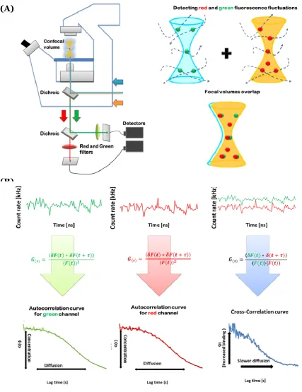
Figure 1-3 Schematic of FCCS experiment.

(A) Confocal Microscope setup with illustration of measurement volume, and (B)

Outline of fluorescence signal analysis. Red and green fluorescent molecules diffuse through the measurement volume generating two fluorescent signals which undergo autocorrelation analysis. Similarity between the fluorescent signals is then determined by cross-correlation analysis. Figure adapted from (Bacia and Schwille, 2003; Barken et al., 2005; Kim et al., 2007; Rarbach et al., 2001).

(A)

10

one position, the RICS approach involves measuring the change in pixel intensity across a fluorescence image acquired by raster scanning. Note that as each pixel intensity is recorded at a different time, temporal information is included in each image. The major advantage of the ICS/RICS approaches is that that they are able to map interactions in the spatial domain. No other method has the capability to measure overall molecular flow in living cells (Hinde et al., 2010).

1.3.4Förster resonance energy transfer and fluorescence lifetime imaging microscopy

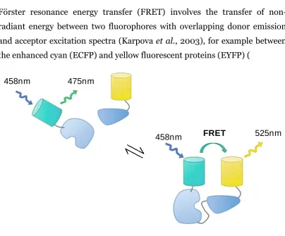
Förster resonance energy transfer (FRET) involves the transfer of non-radiant energy between two fluorophores with overlapping donor emission and acceptor excitation spectra (Karpova et al., 2003), for example between the enhanced cyan (ECFP) and yellow fluorescent proteins (EYFP) (

Figure 1-4). The donor and acceptor are required to be in close proximity (1-10nm) and have a favourable dipole-dipole interaction (Gu et al., 2004; Spiller et al., 2010). This energy transfer allows for the observation of interactions by determining its efficiency, through measuring changes in the intensity of acceptor fluorescence emission or through an associated reduction in donor fluorescence (donor quenching). A key advantage is the

458nm 475nm

525nm

11

ability to observe intra-molecular FRET on dual labelled proteins. This can be extremely informative for studies looking at protein conformation changes (Kajihara et al., 2006).

The interpretation of intensity-based FRET measurements is limited by experimental artefacts such as the relative concentration of the two fluorophores, variations in excitation intensity, and signal spillover. These limitations can be ameliorated by combining FRET with fluorescence lifetime imaging microscopy (FLIM). This method measures the exponential decay rate of the donor emission, which decreases with increased energy transfer from donor to acceptor (FRET) (Suhling et al., 2005). This rate of decay is unaffected by many of the factors that negatively affect intensity-based FRET measurements (Spiller et al., 2010).

(A)

12

Figure 1-4 Principles of FRET.

(A) Fluorescence excitation (broken lines) and emission (solid lines) spectra of ECFP (blue line) and EYFP (blue line). Purple shaded shows efficient overlap facilitating FRET, and orange shaded area shows signal spillover. (B)

Intermolecular FRET between two interacting proteins. Non-interacting proteins are too far away for energy transfer to occur between donor and acceptor fluorophores and therefore no FRET occurs (distance > 10nm), where as interacting proteins might be close enough. Figure adapted from (Hou et al., 2011; Lam et al., 2012).

458nm 475nm

525nm

13

1.4The NF-κB signalling pathway – an exemplar to the systems biology approach

1.4.1Overview

The family of nuclear factor kappa B (NF-κB) transcription factors controls diverse mammalian signalling responses that mediate cell survival, inflammation, and immune response (Gerondakis et al., 1999; Hoffmann et al., 2006; Li and Verma, 2002). The NF-κB network is responsive to a variety of stimuli, including cytokines (Derudder et al., 2003), bacteria-derived products (Covert et al., 2005) and U.V. light (Wu et al., 2004). It has become apparent that the responses of this signalling system to different signals are influenced by complex spatial and temporal dynamics (Ashall et al., 2009; Hoffmann et al., 2002; Nelson et al., 2004). Deciphering the regulatory mechanisms underlying these dynamics is important in order to explain how activation of NF-κB by a variety of signals can lead to stimulus-specific cellular responses.

NF-κB transcription factors exist as dimers of Rel homology domain (RHD) containing proteins (p65/RelA, RelB, c-Rel, and p50/p105 and p52/p100). NF-κB/Rel proteins generate more than 12 dimers recognizing 9–11 nucleotide κB sites. It is most commonly found as a p65:p50 heterodimer (Hoffmann et al., 2002). Both p65 and p50 can also form homodimers, except whilst p65 homodimers are transcriptionally active, p50 homodimers serve to inhibit transcription (Ganchi et al., 1993; Ryseck et al., 1992). Most NF-κB family members can form homo- and heterodimers (in vitro). The exception is RelB, which only forms dimers with p52 and p50 (Dobrzanski et al., 1994; Dobrzanski et al., 1993; Verma et al., 1995).

14

NF-κB’s use the RHD to recognize κB sites in the DNA, only p65, c-Rel, and RelB have transcription activation domains.

The NF-κB dimers are retained in the cytoplasm by the inhibitor κB proteins (IκBα, β, and ε) and NF-κB precursor proteins (p105 and p100) (Gilmore and Herscovitch, 2006; Hoffmann and Baltimore, 2006). Following receptor activation, a signalling cascade is initiated that ultimately converges on the inhibitor kappa B kinase (IKK) complex composed of two highly homologous kinases (IKKα and IKKβ) and a regulatory subunit IKKγ (NEMO) (Perkins, 2007). Following activation, IKK phosphorylates a number of substrates including the IκB’s (Denk et al., 2001; DiDonato et al., 1997) and NF-κB proteinss. The phosphorylation of the IκB’s leads to their subsequent ubiquitination and consequent degradation, allowing for free NF-κB to translocate into the nucleus and potentially activate transcription through specific binding to κB sites. The core network motif of NF-κB is shown in Figure 1-5.

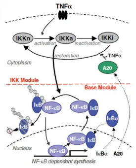
15

Figure 1-5 The core NF-κB signalling system.

16 1.4.2NF-κB as a biological oscillator

The NF-κB system is regulated by negative feedback loops including, but not limited to, IκBα and IκBε (Kearns et al., 2006), and A20 (Lee et al., 2000; Lipniacki et al., 2004). NF-κB activation increases the expression of these genes that are able to remove Rel proteins from the nucleus in the case of the IκB’s, or inhibit the activation of the IKK complex in the case of A20. This two-feedback system has been shown to be able to produce characteristic oscillations in the translocation of NF-κB from the cytoplasm to the nucleus in the case of continuous TNFα stimulation for a variety of cell types (Friedrichsen et al., 2006; Hoffmann et al., 2002; Kearns et al., 2006; Nelson et al., 2004). The ~100 minute period of these oscillations was further found to be robust to a 1000-fold change in the concentration of TNFα (Cheong et al., 2006; Turner et al., 2010).

Cellular rhythms are known to be involved in every aspect of cell physiology, from signalling, motility and development to growth, division and death (Novak and Tyson, 2008). Oscillatory behaviour has been observed across a wide range of frequencies, including from the sub-second range for calcium signalling (Dolmetsch et al., 1997; Dolmetsch et al., 1998), up to 24h for cell cycle and circadian rhythms (Goldbeter, 1995; Tyson and Novak, 2001) Oscillatory dynamics have been quantitatively measured in single cells, cell populations, tissues and whole animals (Paszek et al., 2010a). Cellular rhythms are generated by complex interactions among genes, proteins and metabolites, as well as through the interaction with other oscillators. As a biochemical oscillator, it is likely that some of the functions of NF-κB signalling are synchronised with other oscillatory pathways, and NF-κB is known to interact with components of the cell cycle and p53 for example (Perkins, 2007). Studies have suggested that E2-Factor-1 (E2F-1) might physically associate with p65, and/or its usual dimer partner p50 (Monk, 2003;

Wu et al., 2008). The E2F family of transcription factors are key in cell-cycle

17

from a feedback loop, similar in concept to that of NF-κB, involving the relationship between p53 and its inhibitor MDM2 (Lahav et al., 2004).

18 1.4.3Mathematical modelling of NF-κB 1.4.3.1 Deterministic models of NF-κB

NF-κB is involved in many intra- and inter-cellular signalling processes, with the complex temporal dynamics observed in the NF-κB pathway being believed to determine its role as a regulatory module. In this way, the non-linear NF-κB system has benefited from the application of mathematical modelling, with a variety of stochastic and deterministic models having been produced (Lipniacki and Kimmel, 2007). These models are generally at or below the level of the IKK complex, and involve two-compartment (nucleus and cytoplasm) kinetics of IKK, NF-κB, the IκB’s, their complexes, and mRNA transcripts of A20 and the IκB’s. Fitting parameters proceeds through a mixture of experimental observation and computational inference.

The first model of the pathway to be produced (Hoffmann et al., 2002) was a deterministic model incorporating the three IκB proteins, but not including the A20 negative feedback. The next model produced, by Lipniacki et al. (Lipniacki et al., 2004) provided refinements of the Hoffmann et al. model. Firstly, they better considered the two-compartment kinetics by providing an estimate of the ratio between the nuclear and cytoplasmic volumes. Secondly, IκBα transcription and translation rates were refit to capture the suggestion that the free IκBα constitutes only 15% of total IκBα levels (Rice and Ernst, 1993). The Lipniacki et al. model also gave different consideration towards the NF-κB feedbacks. It did not include IκBβ and IκBε, but instead a single protein labelled ‘IκBα’ models the collective effect of the IκB subtypes. The most fundamental change however was the introduction of the A20 feedback loop. Interestingly, the Lipniacki et al. model makes a prediction on the existence of NF-κB oscillations at the single-cell level.

19

In particular, the use of single-cells presented an opportunity to observe NF-κB translocations under pulsed oscillations of differing periods. Lower frequency pulse stimulations were shown to give repeated full-amplitude translocations, and higher frequency pulses to give reduced-amplitude translocations. A theoretical analysis argued that the structure of the IKK dynamics as implemented in previous models were unable to capture this behaviour and a new model structure proposed. In particular, the production and degradation of active IKK was reconsidered, along with the interaction of A20 with IKK. It is from the Ashall et al. model that most of the modelling work in this thesis begins (Chapter 3).

1.4.3.2 Population vs. single-cell approaches

At the population-level, TNFα induced oscillations of NF-κB are observed to be damped and it is against such data that the Hoffman et al. model was fitted (Hoffmann et al., 2002). The assumption subsequently made was that damped oscillations at the population-level are the result of damped oscillations at the single-cell level. Further to this, the Hoffmann et al. study found that knocking out IκBε results in non-damped oscillations at the population-level, and the subsequent assumption was made that IκBϵ is the cause of the dampening of the oscillations at both the single-cell and population-level.

Damped oscillations were, however, not observed when looking at the single-cell-level in both SK-N-AS cells (Nelson et al., 2004) or MEF cells (Ashall et al., 2009), the cell line used by the Hoffmann et al. study. Instead, asynchronous but robust oscillations were seen. The suggestion made by Ashall et al. is that a deterministic model capturing the limit-cycle behaviour is appropriate for modelling individual cells, but that a model capturing the heterogeneity observed between cells is needed to reproduce data at the population level.

20

are only two copies of the IκBα and A20 feedback genes (Lipniacki et al., 2006). Further to this, although IκBε is known to have a consistent transcriptional delay of 45-min following stimulation (Ashall et al., 2009; Kearns et al., 2006), a gradual population-level increase in IκBε mRNA is also observed (between 30 and 60 min), suggesting a stochastic transcriptional delay. From these suggestions, the Ashall et al. study developed a hybrid, stochastic, three-feedback model on the basis of the their deterministic model structure, which considered delayed stochastic transcription from the IκBϵ gene and stochastic transcription of the IκBα and A20 genes. This model was able to capture the damped oscillations observed at the population level. A further analysis of this model even found that an average delay of 45 min appears to be optimal for inter-cellular heterogeneity, suggesting that population robustness is in fact an essential feature of the NF-κB pathway, providing a mechanism to control the inflammatory response (Paszek et al., 2010b).

1.4.3.3 Limitations of current models of NF-κB

21 1.5Project aims

The primary aim of this thesis is to consider ways in which understanding of the core NF-κB system can be expanded to include a wider array of dynamic interactions. A systems biology approach will be taken, with both theoretical and experimental techniques being explored.

From a modelling perspective, the goal is to consider methods of how the network presented by Ashall et al. can be adapted to incorporate new data on the interactions of NF-κB with other signalling pathways. Simultaneously, methods of expanding the internal dynamics of the Ashall et al. model shall be considered. For both approaches, the main technique will be to explore different network topologies and parameter set spaces in order to elucidate key features of the system structure, and potentially guide experimental work.

22

23 2.1Materials

2.1.1Reagents

Tissue culture medium and non essential amino acids were purchased from Gibco Life Technologies (UK) and Foetal Bovine Serum (FBS) from Harlan Seralab (UK). Human TNFα was supplied by Calbiochem (UK). All other chemicals were supplied by Sigma-Aldrich (UK).

2.1.2Expression vectors

The expression of all mammalian fluorescent protein fusions was under the control of a cytomegalovirus (CMV) immediate-early promoter unless otherwise stated. Neuroblastoma Type-S (SK-N-AS) cells co-expressing p65-DsRedXP and IκBα from stably integrated bacterial artificial chromosomes (BAC) stable cell lines were provided by Dr. A Adamson and Dr. R Awais. SK-N-AS cells expressing Nrf2-VFP from stably integrated bacterial artificial chromosome (BAC) stable cell line was provided by K. Dunn. The characterised transiently expressed expression vectors for E2F1, E2F4, EGFP, and dsRedXp were provided by Dr J. Ankers. The transiently expressed expression vectors for p65 and IκBα have been previously described (Nelson et al., 2004).

2.2Methods

2.2.1Computational modelling and statistics

24 2.2.2Sub-culturing cells

SK-N-AS (ECACC No. 94092302) cells were selected as a well characterised model system for transient and stable fusion protein expression. Cultured as a monolayer and grown in Minimal Essential Medium (MEM) with Earle’s salts, cells were supplemented with 1% non-essential amino acids and 10% FBS and maintained with 5% CO2 at 37ºC. Cells were passaged when the monolayer reached 80% confluency in a 75 cm3 _{tissue culture flask in a final} volume of 20 ml and seeded at ~0.5 x 106_.

Cells were washed with Phosphate Buffered Saline (PBS) then incubated with 1 ml of 0.05% (w/v) trypsin in 0.53 mM EDTA detaching the monolayer from the flask. Cells were resuspended in 9 ml of medium and centrifuged at 200xG for 5 min to remove the trypsin and cell debris. The supernatant was discarded and the cell pellet resuspended in 5 ml of medium. Cells were counted using aTC20 cell counter (BioRad, UK), diluted in medium and seeded at a confluence suitable for transfection and imaging.

2.2.3Transient transfection and imaging

25 2.3Imaging techniques

2.3.1Live cell imaging

Confocal fluorescence microscopy was carried out on transfected cells in glass-bottomed 35mm Greiner dishes in a Ziess XL incubator (37°C, 5% CO2). Two separate imaging systems were used for experiments. The first was a Zeiss LSM710 with Confocor 3 mounted on an Axio observer Z1 microscope with a 63x C-apochromat, 1.2 NA water-immersion objective was typically used for RICS and FCCS data collection. An Argon ion laser and 561nm diode laser were used for imaging with standard wavelengths. The second system was a LSM780 with GaAsp detectors mounted on an Axio observer Z1 microscope with a 63x C-apochromat 1.2 NA water-immersion objective. This system was used for enhanced detection of low expressing constructs such as BAC NRF2 expressing cells. MaiTai Multiphoton laser was used for both multiphoton excitation as well FCS.

2.3.2Dronpa Illumination Strategy

Switching of the photoswitchable fluorophore Dronpa was a manual protocol due to the combination with FCS. Switching Dronpa into the off state was achieved through using the 488nm line from an Argon Ion to simultaneously image and switch Dronpa into the off state. Dronpa was switched on using a 405nm diode laser.

2.3.3FCS and FCCS

26

The lateral beam dimension was estimated to be approximately 229 ± 6.3 nm using Rhodamine 6G as a known calibration standard. A structural parameter value of 5, which is the ratio of the axial to lateral beam dimensions, was assumed. Free EGFP in cells was measured to have a diffusion rate of 48.7 ± 1.8 μm2_s-1_{, agreeing with previous measurements} (Baudendistel et al., 2005; Dross et al., 2009).

The protocols as outlined in Kim et al. (Kim et al., 2007) were followed, with 10 x 10 s runs used for each measurement. The intensity fluctuations recorded and their auto and cross-correlation function calculated in ZEN 2010. Measurements (10x10s) were carried out in cytoplasm or nucleus, with a binning time of 200ns. The data was fitted into a mathematical model describing one, two or three component diffusion; the appropriate model was selected based on the Chi2 _{value describing each fit. The cross-correlation} function included correction for triplet state transitions of fluorophores and assumes Brownian diffusion of molecules. Laser power was typically 1%, but was adjusted as necessary to avoid photobleaching and also to give a suitable count rate with a minimum 0.5kHz counts per molecule (CPM).

2.3.4RICS

RICS was carried out on a Ziess 710 with confocor 3 mounted on an Axio observer Z1 microscope with a 63x C-apochromat, 1.2 NA water-immersion objective. Zen 2010B was used for data collection and analysis. EGFP fluorescence was excited with 488 nm laser light and emission collected between 500 and 530nm dsRedXP was excited with 561 nm laser light and emission collected between 580 and 630nm. Laser power was typically 1%, but was adjusted as necessary to avoid photobleaching to give a high enough fluorescence signal.

27

28

Chapter 3:

Fitting a model of the NF-κB

29 3.1 Introduction

This chapter aims to refit the ordinary differential equation model of NF-κB as presented in the study by Ashall et al. (Ashall et al., 2009), hereafter referred to as the Ashall et al. model. This was motivated by two main aims. The first was the realisation that the Ashall et al. model might be improved by a better representation of the nuclear to cytoplasmic ratio of NF-κB so as to better match imaging data. Following this, there was also the realisation that an improvement could be made in the analysis of the data presented in the Ashall et al. study.

A second motivation came from a study by Lee et al. that found that A20 deficient MEF cells fail to terminate TNFα induced response (Lee et al., 2000). Stimulation by TNFα resulted in a nuclear accumulation of NF-κB, with NF-κB failing to be exported out of the nucleus. An electrophoretic mobility shift assay (EMSA) suggested that nuclear levels of NF-κB in the A20 KO MEFs were comparable to peak nuclear NF-κB levels for wtMEFS. Although the Ashall et al. models include a consideration of the A20 feedback mechanism, it made no attempt to capture the A20 knockout behaviour observed by Lee et al. Given the importance of A20 in determining the oscillatory behaviour of the NF-κB pathway, consideration is here given towards capturing the behaviour observed in A20 deficient cells.

30

31 3.1.1Genetic algorithms

The genetic algorithm approach is a global optimization technique that has gained popularity for the fitting of noisy data. They are global optimization heuristics developed by Holland (Holland, 1975) that are based on an evolutionary paradigm (“survival of the fittest”). A major advantage of genetic algorithms is that they do not require a smooth objective function in contrast to other optimization methods. This is especially useful for fitting biological data. They are also able to escape getting caught in local minima, and so can be successful where other, particularly gradient climbing methods, can fail.

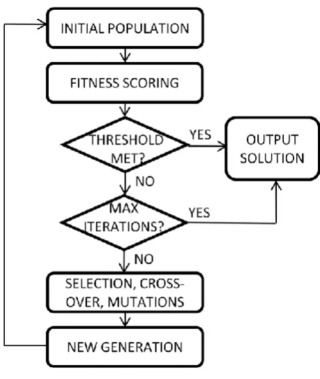
Genetic algorithms are designed to search irregular and poorly understood spaces (Nix and Vose, 1992). Rather than generating a sequence of candidate solutions one at a time (by changing values driving towards an optimum solution) a population of candidate solutions (individuals) is maintained and evolved towards better solutions. Each candidate solution has a set of properties (genotype) which can be mutated and altered. The algorithm begins by first generating a random population of individuals and determining their fitness. The iterative stage is then entered into. To generate a new individual (child), two parents are selected at random, with the selection of an individual as a parent usually being proportional to that individual’s fitness score (“roulette method”). That is, fitter individuals are more likely to be selected for as parents. Then through recombination (crossover) and mutation events, a new individual is generated and its fitness determined. Here selection criteria may or may not be introduced such that, for example, the offspring survives only if it is fitter than at least one other individual. This process repeats until a either convergence criteria or score thresholds are met, or if a maximum number of iterations is reached (Figure 3-1).

32

would begin by randomly selecting a value for each parameter from a defined range. The fitness of each individual would then be calculated using the fitness function, a particular type of objective function that determines how close a simulated curve is to characteristics being fit against. Two individuals are then selected as parents. Various crossover options can be described. In one point crossover, a number the parameters are taken from the first parent and the parameters taken from the second parent, with being chosen at random. In uniform crossover, the choice between two values is made independently on a parameter by parameter basis with some fixed probability, equal to 0.5 for unbiased crossover. A mutation event would be the random assignment of a parameter to a new value (within the defined range of interest), with a parameter value reassignment being dependent on the mutation rate.

Figure 3-1 Schematic of a simple genetic algorithm.

33 3.1.2Sensitivity Analysis

One of the key advantages of building a mathematical description of a biological system is in order to explore parameter sensitivities. A sensitivity score can be defined by (Rand, 2008; Wu et al., 2008),

(3-1)

where represents the parameter that may be varied, the response of the overall system denotes the incremental change in due to the incremental change in . Hence, the sensitivity score of a parameter informs as to how sensitive the response of the system is to a change in a particular parameter. Sensitivity analysis allows the identification of the most significant kinetic reactions which control the dynamic patterns of a biological system (Joo et al., 2007).

There are two broad approaches to sensitivity analysis. Local sensitivity analyses in which single parameters are varied, and global approach in which combinations of parameters are varied. Even with a relatively low number of kinetic variables, a full global sensitivity analysis remains impractical due to the sheer number of parameter combinations available. Yet whilst local sensitivity analyses can be informative in exploring the effect of single point perturbations (e.g. increasing the transcription rate of a gene), they can fail to capture wider aspects of the system. For example, a local sensitivity analysis might identify sensitivity to mRNA production of a feedback gene. However, the ability of that feedback gene to affect the system is likely to be a convolution of mRNA production (and degradation), translation kinetics, transport kinetics, and interaction kinetics. The effect of increased transcription could be compensated for elsewhere in the system.

34

approach. Suppose that a model has kinetic rate variables and we want samples. LHS selects different values from each of kinetic rate variables such that the range of each variable is divided into , non-overlapping intervals on the basis of equal probability. One value from each interval is selected at random with respect to the assumed probability density in the interval. The values thus obtained for the first kinetic rate variable are paired in a random manner (equally likely combinations) with the values of the second kinetic rate variable. These pairs are combined in a random manner with the values of the third kinetic rate variable to form triplets, and so on, until -tuplets are formed.

35 3.2Results

3.2.1Improving the Ashall et al. model

The Ashall et al. model spatially segregates molecular species between nuclear and cytoplasmic cellular compartments. It is formulated in terms of concentration (μM), with molecular concentrations and transport rates being appropriately scaled by , the ratio of the cytoplasmic to nuclear volume in the cell. For example, the following equations describe the fold change in cytoplasmic and nuclear NF-κB protein concentrations with respect to time:

(3-2)

(3-3)

Here the prefixes and correspond to nuclear and phosphorylated species respectively, and constants are as described in Table 3-4. It can be seen in the above equations that scales nuclear import and export in Eq. (3-3) only. As the nucleus has a smaller volume than the cytoplasm, for a given number of molecule numbers, molarity will be greater in the nucleus compared to the cytoplasm. Note that it is assumed that IκBα is not degraded in the nucleus, and so terms involving kt2a and c5a do not appear in Eq. (3-3).

36

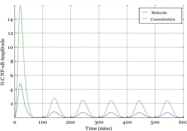
against single-live-cell fluorescent imaging data. These data consist of tracking fluorescently labelled p65 molecules as they translocate into and out of the nucleus, with the change in mean nuclear concentration of NF-κB (i.e. p65) normalised to mean cytoplasmic concentration recorded (N:C). The Ashall et al. model by contrast compares total number of nuclear NF-κB molecules normalised by total cytoplasmic NF-κB molecules, a different measure. This results in the N:C ratio as produced by the model differing from the corresponding experimental N:C ratio by a factor of kv. This difference is illustrated in Figure 3-2 .

Figure 3-2 Comparing molecule number and concentration of N:C ratio of NF-κB output by Ashall et al. model simulation.

‘Molecule’ output corresponds to plot of total nuclear NF-κB molecules divided by total cytoplasmic NF-κB molecules and is the original model output. ‘Concentration’ output corresponds to nuclear NF-κB concentration divided by cytoplasmic NF-κB concentration. Model taken (for continuous TNFα stimulation) from Ashall et al.

0 100 200 300 400 500 600

37

3.2.2Reconsideration of Ashall et al. data

Single-live-cell fluorescent imaging has demonstrated NF-κB oscillations in various cell types (Ashall et al., 2009; Friedrichsen et al., 2006; Nelson et al., 2004). In these studies, translocation dynamics were assessed by dividing the average nuclear fluorescence intensity per pixel for a cell, by its average cytoplasmic fluorescence intensity per pixel (N:C). This was to correct for different levels of expressed fluorescent protein as well as any changes in fluorescence intensity within a time lapse image series due to slight changes in focus, illumination intensity or detector sensitivity. Given the nature of the oscillations observed, between nucleus and cytoplasm, this may seem like a logical choice. Normalisation by mean cytoplasmic signal has, however, the lowest signal-to-noise ratio (Figure 3-3), especially for the first peak. The noise in the normalised signal can be considered by,

(3-4)

38

Figure 3-3 Comparing NF-κB peak amplitudes using different normalisation methods.

Average amplitudes of first three peaks from 25 cells stably transfected with p65-DsRedXP under continuous TNFα stimulation (10 ng/ml). Mean NF-κB nuclear fluorescence signal was normalised(as measured in each cell by the average fluorescent intensity per pixel of P65-dsRedXP) to either the mean total cellular fluorescence (N:T) , mean cytoplasmic fluorescence (N:C), or mean total cell fluorescence at peak 1 (N:T*) (n=25 for each condition). Errors bars represent SD. (Original data taken from Ashall et al.).

A potential problem with the use of the N:T ratio is the necessity of tracking a cell as it migrates and changes shape throughout an entire time course. This can be a computationally intensive process, and may not be possible for certain data sets. Normalisation of data to mean total cell fluorescence taken for a single-frame represents an alternative to tracking total-cell-fluorescence for an entire time course. This requires that the cell remains precisely in focus throughout the course of an experiment, and that there are no photo-bleaching effects, changes in illumination intensity or detector sensitivity. An analysis of 25 cells used in the Ashall et al. study that underwent continuous TNFα treatment, all 25 exhibited no photo-bleaching and 17 were found to exhibit a reasonable drift in total fluorescence intensity (an

0 2 4 6 8 10 12 14 16 18

Peak 1 Peak 2 Peak 3

39

indicator of focal drift). For these cells, mean nuclear fluorescence was normalised to total cell fluorescence at the first peak (N:T*) and a comparison made to the N:T and N:C normalisation methods (Figure 3-3).

Figure 3-4 Change in whole-cell p65-dsRedXP average fluorescence intensity per pixel.

Mean change (across cells) in fluorescence signal over time. Cells (n=6) were from the same field of view imaged every 180 sec over 300 min using automated microscope focus. Errors bars represent SD.

3.2.2.1 Peak detection

In the Ashall et al., the determination of peak timing was by looking for the maximum signal in as a spreadsheet where the fluorescence intensity for each cell in an image series was displayed against the time the image was captured. Here, in order to aid the analysis, a more automated peak detection was utilised. First, the trace of a single cell was smoothed using a 3rd _order moving average such that for the -th data point , obtain

0 0.2 0.4 0.6 0.8 1 1.2 1.4 1.6 1.8 2

0 50 100 150 200 250 300

Fol

d

Fl

u

ores

cen

ce

Int

en

si

ty

40

(3-5)

where is the smoothed data point. At the boundaries, data was smoothed across two points only. In the data range to , peak and trough points were defined to exist if there were data points such that,

.

(3-6)

41

Figure 3-5 Example of cell trace peak detection.

Data taken from a cell stably expressing p65-dsRedXP under continuous TNFα treatment. A 3rd _{order moving average was used to smooth the raw data and this was utilised to detect}

peaks and troughs.

3.2.2.2 NF-κB single-cell pulsatile stimulation data

The protocol for imaging the effects of pulsatile stimulation of TNFα was carried out using cells transiently transfected with a plasmid vector that expressed p65-dsRedXP from a CMV promoter. These experiments were analysed using small region-of-interest (ROI) that were placed in the nucleus or cytoplasm of cells. The ROIs were small circles, from which average intensity per pixel inside the circle was reported by CellTracker software or Zeiss AIM 3.4 software. As such, no excel files containing values for the entire cellular fluorescence levels were available for analysis. The data considered here was collected from time-series images as originally analysed by ex-lab member Dr. Caroline Horton. Note that continuous stimulation data (Figure 3-3) was analysed using whole cell analysis.

0 0.5 1 1.5 2 2.5 3 3.5 4 4.5

0.00 100.00 200.00 300.00 400.00

N:T

R

at

io

of

Re

lA

Time (mins)

42

Figure 3-6 Analysis of P65-dsRedXP translocations in SK-N-AS cells pulsed with TNFα.

SK-N-AS cells transiently transfected with P65dsRedXP were stimulated with TNFα for 5 minutes at either 60- (n=10), 100- (n=34), or 200-(n=21) minute intervals. Mean ROI nuclear fluorescence was normalised by mean ROI cytoplasmic fluorescence at t=0 (N:C0). Values shown are means and error bars represent SD.

An unexpected result was observed upon the reanalysis of the pulsatile stimulation data. In all three conditions, cells appeared to exhibit damped oscillations. A Kruskal-Wallis test was conducted to evaluate the differences in amplitudes between peaks for each of three pulse conditions. A Kruskal-Wallis test is a non-parametric method for testing if samples originate from the same distribution (McDonald, 2009). A significant difference was observed for both the 60-min ( 7.55, 10, 0.023) and 100-min ( 40.29, 25, 0.001) pulse conditions. No significant difference was observed for the 200-min pulse condition, however the calculated -value was close to significant ( 5.96, 21, 0.051). Subsequently, it is assumed for fitting purposes that for all three conditions, a damped response was observed. Note for comparison, a Kruskal-Wallis test applied to

0 0.5 1 1.5 2 2.5 3

Peak 1 Peak 2 Peak 3

N:C

0

NF

-κ

B

Pe

ak

Amp

li

tu

d

e

43

peaks three, four, and five of the continuous TNFα stimulation data found no significant difference in peak amplitudes.

In the original analysis, the nuclear fluorescence was normalised to cytoplasmic fluorescence at each time point. Here, the nuclear signal was normalised by the cytoplasmic signal at time zero, when cytoplasmic signal is maximal. In the original analysis, it was stated that: for the 200-min repeat pulse condition, a complete reset in the system dynamics was observed with all three peak amplitudes being equal; for the 100-min condition, the second and third peaks were equal in amplitude but less than that of the first peak; for the 60-min condition, a dampening of peak amplitudes was observed between peaks. These statements imply that the refractory period of the NF-κB system is approximately 100 min in length, and certainly less than 200 min in length.

The analysis here, by contrast, illustrates that the NF-κB system fails to reset even with 200 min intervals. In fact, the 100-min repeat pulse condition demonstrates the most damping. Comparing the amplitudes of the secondary peak across pulsing conditions, a Kruskal-Wallis test did not show a significant difference ( 5.87, 54, 0.051). However, the value obtained was close to significant and so a post-hoc comparison of means was still carried out using a Tukey test (McDonald, 2009). This found a significant difference only between the 60-min and 100-min secondary peaks. This would suggest that there is a delay in the activity of one of the NF-κB negative feedbacks that is greater than 60 min in length, but less than 100 min in length. The possibility of a delay in A20 activity was thus explored in the refitting of the NF-κB model.

3.2.2.3 NF-κB under continuous TNFα treatment

44

data set was originally generated by Dr Claire Harper, and comes from cells that were stably transfected with a CMV vector expressing labelled p65.

Most strikingly, the first peak amplitude is seen to be only ~3x that of the subsequent oscillation amplitude, contrary to ~5.5x value suggested under the previous analysis. It is apparent in the Ashall et al. model that there is a rapid first dynamic response, with total IκBα degradation occurring in <5 min.

45 (A)

(B)

Figure 3-7 p65 oscillations following TNFα treatment.

(A) Example time courses of ratio of nuclear to total localisation (N:T) of P65-dsRedXP stably transfected into SK-N-AS cells. Single-cell dynamics are shown by different colour lines. (B) Mean and SD of translocation peak amplitudes and peak-to-peak timings. Data is taken from 25 cells (0 failed to respond) imaged for at least 250 min . Data originally generated by Dr. Claire Harper.

0 0.5 1 1.5 2 2.5 3 3.5 4 4.5 5

0 100 200 300 400

N:T R at io of Re lA Time (mins) 0 40 80 120 160 0 1 2 3 4

Peak 1 Peak 2 Peak 3 Peak 4 Peak 5

46

3.2.3Parameter search space and genetic algorithm development 3.2.3.1 Objective function and parameter scoring

Table 3-1 outlines the desired characteristics and values fitted against. For the fitness function (see Section 3.1.1), a score for the -th desired characteristic was defined as,

(3-7)

where is the simulation output, is the characteristic value observed experimentally, and is given by the standard deviation of the experimental data. Note that scores were normalised. Desired characteristics are listed in Table 3-1.

47

Table 3-1– NF-κB time-series features for each TNFα condition

Amplitude refers to nuclear NF-κB normalised by mean total cell fluorescence. Assumed standard deviations are marked with an asterisk (*).

Condition Feature Desired Value

(taken from data)

Continuous

Peak 1 amplitude 2.9 ± 0.83 Limit cycle period 103 ± 29 min Peak 5 / Peak 4 1 ± 0.1* Peak 4 amplitude 1.01 ± 0.53

1.00 ± 0.1*

60-min repeat 5 min pulse

Peak 2 / Peak 1 0.61 ± 0.37 Peak 3 / Peak 1 0.45 ± 0.31

1.00 ± 0.1*

100-min repeat 5 min pulse

Peak 2 / Peak 1 0.48 ± 0.35 Peak 3 / Peak 1 0.24 ± 0.19

1.00 ± 0.1*

200-min repeat 5 min pulse

Peak 2 / Peak 1 0.85± 0.50 Peak 3 / Peak 1 0.60 ± 0.39

1.00 ± 0.1*

48

3.2.3.2Model conversion to number of molecules

Before commencing with parameter refitting, the Ashall et al. model was converted so that species are given in terms of molecule number rather than concentration. In cytoplasmic volume, for a molarity (M), the number of molecules, , is given by,

(3-8)

where is Avogadro’s constant, is the total cell volume (μm3_{), is the} cytoplasmic to nuclear ratio and,

=

. (3-9)

Subsequently, for number of nuclear molecules, , have

49

Converting parameters and initial conditions from units of concentration (units µM or µM−1 _{) to molecule number , have}

(3-11)

where prime notation indicates molecule number. Then converting from concentration ( ) to molecule number ( ) for example, have

50 Which gives,

(3-13)

For equations describing transcription, for example of IκBα, we have

(3-14)

51

Table 3-2– List of model variable names and short description

Variable Description

Active IKK

Inactive IKK

Neutral IKK

Cytoplasmic NF-κB

Nuclear NF-κB

Cytoplasmic IκBα

Nuclear IκBα

Phosphorylated IκBα (cytoplasmic)

A20 protein (cytoplasmic)

IκBα mRNA

A20 mRNA

52

Table 3-3– List of model equations in terms of molecule number

(3-15)

(3-16)

(3-17)

(3-18)

(3-19)

(3-20)

(3-21)

53

(3-23)

(3-24)

(3-25)

(3-26)

(3-27)

54 3.2.3.3 Model scaling

We can now identify which parameters do not need to be fitted by applying appropriate scaling. To remove define,

(3-29)

(3-30)

To remove , define

(3-31)

(3-32)

(3-33)

Similarly, can remove by defining,

(3-34)

(3-35)

(3-36)

55

(3-37)

(3-38)

(3-39) It can also be seen in Eq. (3-26) that can be removed setting,

(3-40)

(3-41)

Finally, it is noted that is a redundant parameter (Eq. (3-22). It is also worth noting that it is possible to define

(3-42)

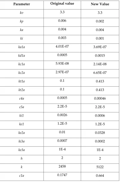
56 3.2.3.4Parameter search space

In total, there are 30 parameters in the Ashall et al. model. Six can be ignored due to appropriate scaling. Six have been determined experimentally or based on reasonable biological assumptions. Seven parameters are constrained experimentally, and 11 remain unconstrained. Hence, there are 18 parameters that are required to be fitted. A symmetric search space is considered by taking the midpoint,

, (3-43)

and calculating the fold change around the midpoint by

, (3-44)