A note on the partially truncated Euler–Maruyama method

A Note on the Partially Truncated

Euler–Maruyama Method

Qian Guo

, Wei Liu

, Xuerong Mao

1

_{Department of Mathematics,}

Shanghai Normal University, Shanghai, China.

2

_{Department of Mathematics and Statistics,}

University of Strathclyde, Glasgow G1 1XH, U.K.

Abstract

The partially truncated Euler–Maruyama (EM) method was recently proposed in our

earlier paper (Guo, Liu, Mao and Yue, 2017) for highly nonlinear stochastic differential

equations (SDEs), where the finite-time strongLr_{-convergence theory was established.}

In this note, we will point out that one condition imposed there is restrictive in the sense

that this condition might force the stepsize to be so small that the partially truncated

EM method would be inapplicable. In this note, we will remove this restrictive condition

but still be able to establish the finite-time strongLr_{-convergence rate. The advantages}

of our new results will be highlighted by the comparisons with our earlier results in (Guo,

Liu, Mao and Yue, 2017).

Key words: Stochastic differential equation, local Lipschitz condition,

Khasminskii-type condition, partially truncated Euler-Maruyama method, convergence rate.

1

Introduction

Influenced by Mao’s papers [8, 9], we recently in [3] developed a new explicit numerical scheme,

called the partially truncated EM method, for nonlinear SDEs under the local Lipschitz

condi-∗_{E-mail:[email protected]}

tion plus the Khasminskii-type condition. The real benefits of this new method lie in that the

method can well preserve the asymptotic stability and boundedness of the underlying SDEs.

However, we will point out in Section 2 that one condition imposed in [3] is restrictive in the

sense that this condition might force the stepsize to be so small that the partially truncated

EM method would be inapplicable. In this note, we will remove this restrictive condition but

still be able to establish the finite-time strong Lr_{-convergence rate.}

As this is the continuation of our earlier paper [3], we will use the same notation as used

there. We will only list and cite some necessary references here but the reader can find more

in [3].

2

Motivation

In this section, we will point out that one condition imposed in [3] is restrictive in the sense

that this condition might force the stepsize to be so small that the partially truncated EM

method would be inapplicable. For this purpose, we need to make a quick review on the

partially truncated EM method. Consider a d-dimensional SDE

dx(t) =f(x(t))dt+g(x(t))dB(t) (2.1)

on t ≥ 0 with the initial value x(0) = x0 ∈ Rd, where B(t) is an m-dimensional Brownian

motion,f :_Rd→_Rd _{and g :}

Rd→Rd×m.We assume that f and g can be decomposed as

f(x) = F1(x) +F(x) and g(x) =G1(x) +G(x), (2.2)

where F1, F : Rd → Rd and G1, G : Rd → Rd×m are all Borel measurable. The assumptions

imposed in [3] are listed below.

Assumption 2.1 Assume that there are constants L1 >0 and γ ≥0 such that

|F1(x)−F1(y)| ∨ |G1(x)−G1(y)| ≤L1|x−y| (2.3)

and

|F(x)−F(y)| ∨ |G(x)−G(y)| ≤L1(1 +|x|γ+|y|γ)|x−y| (2.4)

Assumption 2.2 Assume that there is a pair of constants r >¯ 2 and L2 such that

(x−y)T(F(x)−F(y)) + ¯r−1

2 |G(x)−G(y)|

2 _≤L

2|x−y|2 (2.5)

for all x, y ∈_Rd_.

Assumption 2.3 Assume that there are constants p >¯ r¯and K2 >0 such that

xTF(x) + p¯−1 2 |G(x)|

2 _≤K

2(1 +|x|2) (2.6)

for all x∈_Rd_.

As pointed out in [3], (2.6) cannot be deduced from (2.5) as we need ¯p >r¯. Moreover, we

observe from (2.3) that the coefficients F1 andG1 satisfy the linear growth condition, namely

there exists a constant K1 >0 such that

|F1(x)| ∨ |G1(x)| ≤K1(1 +|x|) (2.7)

for all x∈_Rd_.

To define the partially truncated EM numerical solutions, we first choose a strictly

in-creasing continuous function µ:_R+ →R+ such that µ(u)→ ∞ asu→ ∞ and

sup

|x|≤u

|F(x)| ∨ |G(x)|

≤µ(u), ∀u≥1. (2.8)

Denote byµ−1 the inverse function ofµand we see thatµ−1 is a strictly increasing continuous function from [µ(0),∞) to_R+. We also choose a strictly decreasing functionh: (0,1]→(0,∞)

and a constant ¯h≥1 such that

lim

∆→0h(∆) =∞ and ∆ 1/4

h(∆)≤¯h, ∀∆∈(0,1]. (2.9)

Before we proceed, let us make an useful remark.

Remark 2.4 In [3] where the partially truncated EM was originally developed, it was required

to choose a number ∆∗ ∈ (0,1] and a strictly decreasing function h : (0,∆∗] → (0,∞) such that

h(∆∗)≥µ(1), lim

∆→0h(∆) =∞ and ∆ 1/4

h(∆) ≤1, ∀∆∈(0,1).

do not make any effect on the results in [3]. In fact, the condition h(∆∗)≥µ(1) was only used to show [3, Lemma 2.5] (followed from [8]). Instead of [3, Lemma 2.5], we will have our new

Lemma 3.2. Comparing these two lemmas, we observe that the constant 2K2 in [3, Lemma

2.5] is now replaced by K4 in our our new Lemma 3.2. But this change does not have any

effect on the results in [3]. We can also check that replacing ∆1/4h(∆) ≤1 by ∆1/4h(∆)≤ ¯h

does not make any effect on the proof of [3, Lemma 3.2],which we will cite as Lemma 3.3 in

this paper (in fact, such a change does not make any effect on any result in [3]).

For a given stepsize ∆ ∈(0,1], let us define the mappingπ∆ :Rd →Rd by

π∆(x) = (|x| ∧µ−1(h(∆)))

x

|x|,

where we set x/|x|= 0 when x= 0. We then define the truncated functions

F∆(x) =F(π∆(x)) and G∆(x) =G(π∆(x)) (2.10)

for x∈_Rd_{. It is easy to see that}

|F∆(x)| ∨ |G∆(x)| ≤µ(µ−1(h(∆))) =h(∆) ∀x∈Rd. (2.11)

From now on we will define

f∆(x) = F1(x) +F∆(x) and g∆(x) =G1(x) +G∆(x). (2.12)

The discrete-time partially truncated EM numerical solutionsX∆(tk)≈x(tk) fortk =k∆

are formed by setting X∆(0) =x0 and computing

X∆(tk+1) =X∆(tk) +f∆(X∆(tk))∆ +g∆(X∆(tk))∆Bk, (2.13)

fork = 0,1,· · ·, where ∆Bk =B(tk+1)−B(tk). There are two versions of the continuous-time

truncated EM solutions. The first one is defined by

¯

x∆(t) =

∞

X

k=0

X∆(tk)I[tk,tk+1)(t), t ≥0, (2.14)

where throughout this paper ID denotes the indicator function of set D. This is a simple step

process so its sample paths are not continuous. We will refer to this as the continuous-time

step-process partially truncated EM solution. The other one is defined by

x∆(t) =x0+

Z t

0

f∆(¯x∆(s))ds+

Z t

0

for t ≥0. We will refer to this as the continuous-time continuous-sample partially truncated

EM solution. We observe thatx∆(tk) = ¯x∆(tk) = X∆(tk) for all k ≥0. Moreover, x∆(t) is an

Itˆo process with its Itˆo differential

dx∆(t) = f∆(¯x∆(t))dt+g∆(¯x∆(t))dB(t). (2.16)

The following theorem is one of the main results in [3].

Theorem 2.5 ([3, Theorem 3.1]) Let Assumptions 2.1, 2.2 and 2.3 hold and let T > 0 be

arbitrary. If p∈(¯r,p¯), 2p >rγ¯ and for r∈[2,r¯)

h(∆)≥µ((∆r/2(h(∆))r)−1/(p−r)), (2.17)

then there is a ∆¯ ∈(0,∆∗] such that for all ∆∈(0,∆]¯

E|x∆(T)−x(T)|r≤C∆r/2(h(∆))r (2.18) and

E|x¯∆(T)−x(T)|r ≤C∆r/2(h(∆))r, (2.19) where throughout this paper C stands for generic positive real constants.

Let us now explain, via an example, that condition (2.17) is somehow restrictive as it

might force the stepsize to be so small that the partially truncated EM method would be

inapplicable. Consider the scalar power logistic model in a population system (see, e.g., [1])

dx(t) = x(t)[(5−10x2(t))dt+x(t)dB(t)], (2.20)

whereB(t) is a scalar Brownian motion. Naturally, we can decompose the coefficientsf(x) =

5x−10x3 _{and g(x) = x}2 _{in the form of (2.2) with}

F1(x) = 5x, F(x) =−10x3, G1(x) = 0, G(x) = x2.

Obviously, (2.3) is satisfied byF1 and G1, while it is easy to verify

|F(x)−F(y)| ∨ |G(x)−G(y)| ≤15|x−y|(1 +x2+y2), ∀x, y ∈_R.

Thus, Assumption 2.1 is satisfied with γ = 2. It is also not difficult to show that for ¯r= 3,

(x−y)(F(x)−F(y)) + r¯−1

2 |G(x)−G(y)|

2 _≤

whence Assumption 2.2 is satisfied with ¯r = 3. Moreover, for ¯p= 21,

xF(x) + p¯−1 2 |G(x)|

2 _{= 0, ∀x,∈}

R,

so Assumption 2.3 is satisfied with ¯p= 21. Furthermore, we have

sup

|x|≤u

|F(x)| ∨ |G(x)|

≤10u3, ∀u≥1,

whence we can choose µ(u) = 10u3. Finally choose h(∆) = ∆−1/6 which meets condition (2.9). Then, for r = 2 andp= 20, condition (2.17) becomes

∆−1/6 ≥10∆−1/9, namely ∆≤10−18. (2.21)

This means we have to use an extremely small stepsize in order to apply Theorem 2.5 but this

is not realistic. It is therefore very useful to remove this restrictive condition (2.17) and this

is the main driven force for us to write this note.

3

Main Results

3.1

Convergence rate

It was shown in [3] that under Assumptions 2.1 and 2.3, for anyp∈(2,p¯),

xTf(x) + p−1 2 |g(x)|

2 _≤

K3(1 +|x|2) (3.1)

for all x∈_Rd_{, where}

K3 = 2K1+K2 +

K2

1(p−1)(¯p−1)

¯

p−p .

It was also shown in [3] that under Assumptions 2.1 and 2.2, for any q∈(2,¯r)

(x−y)T(f(x)−f(y)) + q−1

2 |g(x)−g(y)|

2 _≤L

3|x−y|2, (3.2)

where

L3 = 2L1+L2+

L2

1(q−1)(¯r−1)

¯

r−q .

The following lemma is therefore well known (see, e.g., [5, 7, 11]).

Lemma 3.1 Under Assumptions 2.1 and 2.3, the SDE (2.1) has a unique global solution x(t)

and, moreover, for any p∈(2,p¯),

sup

0≤t≤T E

The following lemma shows that the truncated functionsF∆andG∆preserve Assumption

2.3 very well.

Lemma 3.2 Let Assumption 2.3 hold. Then, for all ∆∈(0,1], we have

xTF∆(x) +

¯

p−1

2 |G∆(x)|

2 _≤K

4(1 +|x|2), ∀x∈Rd, (3.4) where K4 = 2K2 1∨[1/µ−1(h(1))]

.

Proof. This lemma was essentially proved in [3, 8] but we here do not need conditionh(∆∗)≥

µ(1) as we pointed out in Remark 2.4.

Fix any ∆ ∈ (0,1]. For x ∈ _Rd _{with |x| ≤ µ}−1_{(h(∆)), the required assertion (3.4) holds}

clearly. For x∈_Rd _{with |x|> µ}−1_{(h(∆)), the proof of [8, Lemma 2.4] shows that}

xTF∆(x) +

¯

p−1

2 |G∆(x)|

2 _≤ |x|

µ−1_(h(∆))K2(1 + [µ

−1_(h(∆))]2_).

Noting that µ−1_{(h(∆))≥µ}−1_{(h(1)), we then derive}

xTF∆(x) +

¯

p−1

2 |G∆(x)|

2 _≤K

2|x|

1

µ−1_(h(1)) +|x|

≤ K2 1∨[1/µ−1(h(1))]

(|x|+|x|2_)≤0.5K

4(1 + 2|x|2)≤K4(1 +|x|2)

as required. 2

As we explained in Remark 2.4, this lemma plays the same role as [3, Lemma 2.5] did and

all the results in [3] work although our new condition (2.9) on the function h(·) is simpler. In

particular, we can then cite a lemma from [3] for the use of this paper.

Lemma 3.3 Let Assumptions 2.1 and 2.3 hold. Let p∈(2,p¯) and T > 0 be arbitrary. Then

sup

0<∆≤1

sup

0≤t≤TE

|x∆(t)|p ≤C. (3.5)

(We emphasise once again that C stands for generic positive real constants dependent on

T,p, p, x¯ 0,K1, K2,¯hetc. but independent of∆and its values may change between occurrences.)

The following lemma was essentially proved in [3].

Lemma 3.4 Let Assumptions 2.1 and 2.3 hold. Let p∈(0,p¯) andT > 0be arbitrary. Then,

for every ∆∈(0,1],

Proof. This lemma was proved in [3] for p∈(2,p¯) in the sense that there is a ¯∆∈(0,1] such

that assertion (3.6) holds for all ∆∈(0,∆]. Our new version here is therefore an improvement¯

of that in [3]. It is sufficient to show our lemma for p ∈ (2,p¯) as the assertion for p ∈ (0,2]

follows then from the H¨older inequality. We hence fix p ∈ (2,p¯) arbitrarily. It follows from

Lemma 3.3 that

sup

0<∆≤1

sup

0≤t≤TE

|x∆(t)|p ≤C(h(1))p. (3.7)

Now, fix any ∆ ∈ (0,1]. For any t ∈ [0, T], there is a unique k ≥ 0 such that tk ≤ t ≤ tk+1.

By (2.7) and (2.11), it is easy to show from (2.15) that

E|x∆(t)−x¯∆(t)|p ≤C∆p/2

1 +_E|x¯∆(t)|p+ (h(∆))p

. (3.8)

But, by (3.7) and the decreasing property of h,

E|x¯∆(t)|p ≤C(h(1))p ≤C(h(∆))p.

We hence get assertion (3.6) from (3.8). 2

Let us now present one more lemma which will be used in the proof of our main theorem

later.

Lemma 3.5 Let Assumption 2.1 hold. Then

|f(x)−f(y)| ∨ |g(x)−g(y)| ≤2L1(1 +|x|γ+|y|γ)|x−y| (3.9)

for all x, y ∈_Rd_{. Moreover, for any ∆∈(0,1],}

|f∆(x)−f∆(y)| ∨ |g∆(x)−g∆(y)| ≤2L1(1 +|x|γ+|y|γ)|x−y| (3.10)

for all x, y ∈_Rd_.

Proof. Assertion (3.9) follows easily from Assumption 2.1. To show assertion (3.10), we first

show that the truncated functions F∆ and G∆ preserve condition (2.4) perfectly. In fact, by

condition (2.4) , we have

|F∆(x)−F∆(y)| ∨ |G∆(x)−G∆(y)|

= |F(π∆(x))−F(π∆(y))| ∨ |G(π∆(x))−G(π∆(y))|

for all x, y ∈_Rd_{. Noting}

|π∆(x)| ≤ |x|, |π∆(y)| ≤ |y|, |π∆(x)−π∆(y)| ≤ |x−y|,

we get

|F∆(x)−F∆(y)| ∨ |G∆(x)−G∆(y)| ≤L1(1 +|x|γ+|y|γ)|x−y|. (3.11)

This, together with condition (2.3), implies the other assertion (3.10). 2

Moreover, we also observe from Assumption 2.1 that

|F(x)| ∨ |G(x)| ≤L4|x|(1+γ), ∀|x| ≥1, (3.12)

where L4 = 2L1+|F(0)|+|G(0)|.

The following theorem is our main result in this paper which shows the rate of Lr

-convergence. From now on, we will fix T >0 arbitrarily.

Theorem 3.6 Let Assumptions 2.1, 2.2, 2.3 hold and assume that there is a numberp∈(2,p¯)

such that

p > (1 +γ)¯r. (3.13)

Let r ∈[2,r¯) be arbitrary. Then for any ∆∈(0,1],

E|x(T)−x∆(T)|r ≤C

(µ−1(h(∆)))−(p−(1+γ)r)+ ∆r/2(h(∆))r

(3.14)

and

E|x(T)−x¯∆(T)|r ≤C

(µ−1(h(∆)))−(p−(1+γ)r)+ ∆r/2(h(∆))r. (3.15)

In particular, recalling (3.12), we may define

µ(u) =L4u(1+γ), u≥0, (3.16)

and let

h(∆) = ¯h∆−ε for some ε∈(0,1/4] (3.17)

to get

E|x(T)−x∆(T)|r ≤C ∆[ε(p−(1+γ)r)/(1+γ)]∧[r(1−2ε)/2] (3.18) and

Proof. First of all, fix a number q∈(r,r¯). By (3.13), we have

p > (1 +γ)q. (3.20)

We also fix ∆∈(0,1] arbitrarily. Letζ∆(t) = x(t)−x∆(t) fort≥0. For each integer n >|x0|,

define the stopping time

ρn = inf{t ≥0 :|x(t)| ∨ |x∆(t)| ≥n},

where we set inf∅=∞ (as usual ∅ denotes the empty set). By the Itˆo formula, we have that

for 0≤t≤T,

E|ζ∆(t∧ρn)|r ≤ E

Z t∧ρn

0

r|ζ∆(s)|r−2

ζ_∆T(s)[f(x(s))−f∆(¯x∆(s))]

+r−1

2 |g(x(s))−g∆(¯x∆(s))|

2

ds. (3.21)

Noting

r−1

2 |g(x(s))−g∆(¯x∆(s))|

2

≤ r−1

2

h

1 + q−r

r−1

|g(x(s))−g(x∆(s))|2+

1 + r−1

q−r

|g(x∆(s))−g∆(¯x∆(s))|2 i

= q−1

2 |g(x(s))−g(x∆(s))|

2₊(r−1)(q−1)

2(q−r) |g(x∆(s))−g(¯x∆(s))|

2_,

we get from (3.21) that

E|ζ∆(t∧ρn)|r ≤H1+H2, (3.22)

where

H1 =E

Z t∧ρn

0

r|ζ∆(s)|r−2

ζ_∆T(s)[f(x(s))−f(x∆(s))]

+ q−1

2 |g(x(s))−g(x∆(s))|

2_{ds (3.23)}

and

H2 =E

Z t∧ρn

0

r|ζ∆(s)|r−2

ζ_∆T(s)[f(x∆(s))−f∆(¯x∆(s))]

+ (r−1)(q−1)

2(q−r) |g(x∆(s))−g∆(¯x∆(s))|

2_{ds. (3.24)}

By (3.2), we have

H1 ≤rL3E

Z t∧ρn

0

It is also easy to see that

H2 ≤H3+H4, (3.26)

where

H3 =E

Z t∧ρn

0

r|ζ∆(s)|r−2

ζ_∆T(s)[f(x∆(s))−f∆(x∆(s))]

+(r−1)(q−1)

(q−r) |g(x∆(s))−g∆(x∆(s))|

2_ds

and

H4 =E

Z t∧ρn

0

r|ζ∆(s)|r−2

ζ_∆T(s)[f∆(x∆(s))−f∆(¯x∆(s))]

+(r−1)(q−1)

(q−r) |g∆(x∆(s))−g∆(¯x∆(s))|

2_ds.

Let us estimate H4 first. By (3.10), we have

H4 ≤E

Z t∧ρn

0

r|ζ∆(s)|r−2

0.5|ζ∆(s)|2+ 0.5|f∆(x∆(s))−f∆(¯x∆(s))|2

+ (r−1)(q−1)

(q−r) |g∆(x∆(s))−g∆(¯x∆(s))|

2_ds

≤0.5r_E

Z t∧ρn

0

|ζ∆(s)|rds

+C_E

Z t∧ρn

0

|ζ∆(s)|r−2(1 +|x∆(s)|2γ+|x¯∆(s)|2γ)|x∆(s)−x¯∆(s)|2ds. (3.27)

But, by the well-known Young inequality (see, e.g., [10, p.52]),

|ζ∆(s)|r−2(1 +|x∆(s)|2γ+|x¯∆(s)|2γ)|x∆(s)−x¯∆(s)|2

≤r−2

r |ζ∆(s)|

r

+ 2

r(1 +|x∆(s)|

2γ

+|x¯∆(s)|2γ)r/2|x∆(s)−x¯∆(s)|r

≤|ζ∆(s)|r+C(1 +|x∆(s)|γr+|x¯∆(s)|γr)|x∆(s)−x¯∆(s)|r.

Substituting this into (3.27) yields

H4 ≤CE

Z t∧ρn

0

|ζ∆(s)|rds

+C

Z T

0

E

(1 +|x∆(s)|γr+|x¯∆(s)|γr)|x∆(s)−x¯∆(s)|r

ds. (3.28)

By the H¨older inequality,

E

(1 +|x∆(s)|γr+|x¯∆(s)|γr)|x∆(s)−x¯∆(s)|r

≤3γr(p−1)/p _E(1 +|x∆(s)|p+|x¯∆(s)|p)

γr/p

E|x∆(s)−x¯∆(s)|pr/(p−γr)

(p−γr)/p

But, by (3.20), we have p > (1 +γ)r and hence pr/(p−γr) < p. So we can apply Lemmas

3.3 and 3.4 to get

E

(1 +|x∆(s)|γr+|x¯∆(s)|γr)|x∆(s)−x¯∆(s)|r

≤C∆r/2(h(∆))r.

Substituting this into (3.28) gives

H4 ≤E

Z t∧ρn

0

|ζ∆(s)|rds+C∆r/2(h(∆))r. (3.29)

Let us now estimate H3. It is easy to show that

H3 ≤CE

Z t∧ρn

0

|ζ∆(s)|rds+H5, (3.30)

where

H5 =C

Z T

0

E|f(x∆(s))−f∆(x∆(s))|r+E|g(x∆(s))−g∆(x∆(s))|r

ds. (3.31)

Recalling (2.2), (2.12) and (2.10), we see

E|f(x∆(s))−f∆(x∆(s))|r =E|F(x∆(s))−F∆(x∆(s))|r=E|F(x∆(s))−F(π∆(x∆(s)))|r.

By (2.4), the H¨older inequality and Lemma 3.3, we then derive

E|f(x∆(s))−f∆(x∆(s))|r

≤C _E(1 +|x∆(s)|γr+|π∆(x∆(s))|γr)|x∆(s)−π∆(x∆(s))|r

≤C_E(1 +|x∆(s)|p+|π∆(x∆(s))|p)

γr/p

E|x∆(s)−π∆(x∆(s))|pr/(p−γr)

(p−γr)/p

≤C_EhI{|x∆(s)|>µ−1(h(∆))}|x∆(s)|

pr/(p−γr)i(p−γr)/p

≤Ch_P{|x∆(s)|> µ−1(h(∆))}

i(p−(1+γ)r)/(p−γr)h

E|x∆(s)|p

ir/(p−γr)(p−γr)/p

≤C

_E|x_∆(s)|p

(µ−1_(h(∆)))p

(p−(1+γ)r)/p

≤C(µ−1(h(∆)))−(p−(1+γ)r).

Similarly, we can show

E|g(x∆(s))−g∆(x∆(s))|r ≤C(µ−1(h(∆)))−(p−(1+γ)r).

Substituting the two inequalities into (3.31) and then putting the resulting inequality into

(3.30), we obtain

H3 ≤CE

Z t∧ρn

0

Combining (3.22), (3.25), (3.26, (3.29) and (3.32) together we get

E|ζ∆(t∧ρn)|r ≤ C_E

Z t∧ρn

0

|ζ∆(s)|rds+ (µ−1(h(∆)))−(p−(1+γ)r)+ ∆r/2(h(∆))r

≤ C

Z t

0

E|ζ∆(s∧ρn)|rds+ (µ−1(h(∆)))−(p−(1+γ)r)+ ∆r/2(h(∆))r

. (3.33)

An application of the Gronwall inequality yields that

E|ζ∆(T ∧ρn)|r ≤C

(µ−1(h(∆)))−(p−(1+γ)r)+ ∆r/2(h(∆))r.

This implies the desired assertion (3.14) by letting n → ∞. The another assertion (3.15)

follows from (3.14) and Lemma 3.4.

Finally, when µ is defined by (3.16), then µ−1_{(u) = (u/L}

4)1/(1+γ). Substituting this and

(3.17) into (3.14) we get

E|x(T)−x∆(T)|r ≤C

∆ε(p−(1+γ)r)/(1+γ)+ ∆r(1−2ε)/2,

which is the required assertion (3.18). Similarly, we can show (3.19). The proof is therefore

complete. 2

The following corollary shows that the order of Lr_{-convergence is close to 1/2. This is}

almost optimal if we recall that the classical EM method has order 1/2 of Lr-convergence under the global Lipschitz condition.

Corollary 3.7 Let Assumptions 2.1, 2.2 hold and let Assumption 2.3 hold for any p >¯ r¯. Let

µ(·) and h(·) be defined by (3.16) and (3.17). Then, for any r∈[2,r¯) and any ε∈(0,1/4),

E|x(T)−x∆(T)|r ≤C∆r(1−2ε)/2 (3.34) and

E|x(T)−x¯∆(T)|r ≤C∆r(1−2ε)/2. (3.35) Proof. Choosing p sufficiently large for

ε(p−(1 +γ)r)/(1 +γ)> r(1−2ε)/2,

we get the assertions from (3.18) and (3.19). 2

Let us discuss an example to illustrate this corollary before we make a comparison between

Example 3.8 Consider the scalar stochastic Ginzburgh–Landau equation (see, e.g., [2, 6])

dx(t) = (ax(t)−bx3(t))dt+cx(t)dB(t), (3.36)

where B(t) is a scalar Brownian motion and a, b, c are three positive numbers. We naturally

decompose the coefficientsf(x) =ax−bx3 _{and g(x) =cx in the form of (2.2) with}

F1(x) = ax, F(x) = bx3, G1(x) = cx, G(x) = 0

for x ∈ _R. Both F1(x) and G1(x) are linear functions of x so they satisfy condition (2.3) of

course. Also, for x, y ∈_R,

|F(x)−F(y)|=b(x2+xy+y2)|x−y| ≤2b(x2+y2)|x−y|.

Thus, Assumption 2.1 is satisfied with γ = 2 as G(x) = 0. Moreover, for any ¯r >2

(x−y)(F(x)−F(y)) + r¯−1

2 |G(x)−G(y)|

2 _=−b(x2_+xy+y2_)(x−y)2 _≤0.

This means that Assumption 2.2 holds for any ¯r >2. Furthermore, for any ¯p > 2,

xF(x) + p¯−1 2 |G(x)|

2 _=−bx4 _≤0.

Hence, Assumption 2.3 is also satisfied for any ¯p >2. To apply Corollary 3.7, we still need to

design functionsµ and h. Noting that

sup

|x|≤u

(|F(x)| ∨ |G(x)|)≤(b∨c)u3, ∀u≥1,

we can have µ(u) = (b∨v)u3 and its inverse function µ−1(u) = (u/(b∨c))1/3 for u≥ 0. For

ε ∈ (0,1/4], we define h(∆) = ¯h∆−ε _{for ∆ > 0. Obviously, (2.9) holds. We can therefore}

conclude by Corollary 3.7 that for anyr ≥2, the partially truncated EM solutions of the SDE

(3.36) satisfy

E|x(T)−x∆(T)|r ≤C∆r(1−2ε)/2 and E|x(T)−x¯∆(T)|r ≤C(∆r(1−2ε)/2).

That is, the order of Lr_{-convergence can be arbitrarily close to 1/2.}

3.2

Comparison

It is time to compare our new Theorem 3.6 with our earlier result, namely Theorem 2.5.

Although both theorems are formed under the same set of assumptions (i.e., Assumptions 2.1,

• Theorem 3.6 does not need condition (2.17) in Theorem 2.5.

• The assertions of Theorem 3.6 hold for any ∆∈ (0,1] while the assertions of Theorem

2.5 holds only for sufficiently small ∆ which satisfies condition (2.17).

• Condition p >(1 +γ)¯r in Theorem 3.6 is stronger than 2p > γr¯in Theorem 2.5.

• The convergence order showed by Theorem 3.6 is worse than that by Theorem 2.5,

although could be the same when p is sufficiently large as Corollary 3.7 has shown.

The key advantage of our new Theorem 3.6 lies in that it does not need condition (2.17).

We have already seen in Section 2 that condition (2.17) could sometimes make Theorem 2.5

inapplicable.

Example 3.9 Let us return to the SDE (2.20) and show that our new Theorem 3.6 is indeed

applicable. We have already verified that Assumptions 2.1, 2.2 and 2.3 hold withγ = 2, ¯r= 3

and ¯p= 21. We also have µ(u) = 3u3.

Let us first let h(∆) = ∆−1/5. For r = 2 andp= 20, condition (2.17) becomes

∆−1/5 ≥10−1/10, namely ∆≤10−10,

and Theorem 2.5 shows that the partially truncated EM method applied to the SDE (2.20)

has the property that

E|x(T)−x∆(T)|2∨E|x(T)−x¯∆(T)|2 ≤C∆3/5. (3.37)

On the other hand, all the conditions of our new Theorem 3.6 are satisfied and hence we can

conclude that

E|x(T)−x∆(T)|2∨E|x(T)−x¯∆(T)|2 ≤C(∆14/15+ ∆3/5)≤C∆3/5 (3.38)

for any stepsize ∆ ∈ (0,1]. This shows the same convergence rate as (3.37) did but we have

no longer required ∆≤10−10_.

To improve the convergence rate, let us choose h(∆) = ∆−1/6_{. Again, let r = 2 and}

p = 20. We already showed in Section 2 that condition (2.17) forces ∆ ≤ 10−18_{. In this}

situation, Theorem 2.5 shows

But, applying Theorem 3.6 we get

E|x(T)−x∆(T)|2∨E|x(T)−x¯∆(T)|2 ≤C(∆7/9+ ∆2/3)≤C∆2/3. (3.40)

for any stepsize ∆∈(0,1]. In other words, our new Theorem 3.6 shows the same convergence

rate as Theorem 2.5 did without the unrealistic condition ∆≤10−18_.

Let us discuss one 2-dimensional example to illustrate our theory further.

Example 3.10 Consider a 2-dimensional stochastic Lotka-Volterra system described by

dx(t) = diag(x1(t), x2(t))[b+Ax2(t)]dt+σx(t)dB(t), (3.41)

where xs(t) = (xs₁(t), xs₂(t))T for any s ≥1,b = (b1, b2)T,σ ∈R2×2,

A=





−1 −1

−1 −1



.

We naturally decompose the coefficients into f(x) =F1(x) +F(x) and g(x) = G1(x) +G(x)

with

F1(x) = (b1x1, b2x2)T, F(x) = (ϕ1(x), ϕ2(x))T, G1(x) =σx, G(x) = 0,

where

ϕi(x) =

2 X

j=1

aijxix2j, 1≤i≤2.

As both F1(x) andG1(x) are linear functions of x, they of course satisfy condition (2.3). For

x, y ∈_R2_{, noting}

ϕi(x)−ϕi(y) =

2 X

j=1

aij(xix2j −yiyj2) =

2 X

j=1

aij[xi(x2j −y

2

j) + (xi−yi)y2j],

we see that there is a positive constant L1 such that

|F(x)−F(y)| ≤L1(1 +|x|2+|y|2)|x−y|.

derive that

(x−y)T(F(x)−F(y)) =−(x−y)T(x|x|2_−y|y|2₎

=−(x−y)T((x−y)|x|2_+y|x|2_−x|y|2_{+ (x−y)|y|}2₎

=−(|x−y|2_−xT_y)(|x|2_+|y|2_{) + 2|x|}2_|y|2

=− 1

2|x−y|

2

(|x|2+|y|2)− 1

2(|x|

2

+|y|2)2+ 2|x|2|y|2

=− 1

2|x−y|

2

(|x|2+|y|2)− 1

2(|x|

2_{− |}

y|2)2

≤0.

This means that Assumption 2.2 holds for any ¯r >2. Meanwhile, for any ¯p >2,

xF(x) + p¯−1 2 |G(x)|

2 _{= (x}2₎T_Ax2 _≤0.

Thus, Assumption 2.3 is satisfied. Noting that

sup

|x|≤u

(|F(x)| ∨ |G(x)|)≤(|A|F ∨σ)u3, ∀u≥1,

which leads µ(u) = (3∨σ)u3_{. By using the same method in Example 3.8, we conclude that}

the order of Lr-convergence can be arbitrarily close to 1/2 for any r≥2.

4

Numerical Example

The convergence rate of the partially truncated EM method was illustrated in [3] by the

following example.

Example 4.1 Consider a nonlinear SDE described by

dx(t) = (x(t)−x5(t))dt+x2(t)dB(t), t≥0, (4.1)

with the initial value x(0) = 1.

To our best knowledge, the fully tamed EM method (see [4]) defined by

Xi+1 =Xi+

f(Xi)∆ +g(Xi)∆Bi

max{1,∆|f(Xi)∆ +g(Xi)∆Bi|}

,

is also developed for SDEs with both drift and diffusion coefficients growing super-linearly.

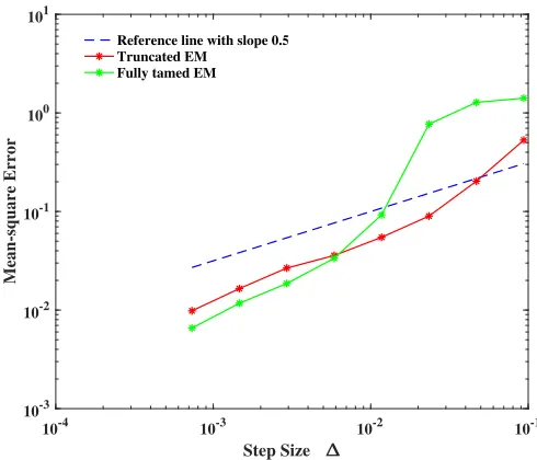
10-4 10-3 10-2 10-1

Step Size

10-3 10-2 10-1 100 101

Mean-square Error

Reference line with slope 0.5 Truncated EM

Fully tamed EM

Figure 1: The strong convergence rate at the terminal timeT = 3.

simulate 10,000 sample paths to test the mean-square error. We regard the numerical solutions

generated by the partially truncated EM method and the fully tamed EM method in interval

[0,3] with the very small step size ∆ = 2−12 as the ‘exact solutions’, respectively. Figure 1 displays the L2 _{errors of the fully tamed EM method and the partially truncated EM method}

at the terminal time T = 3. It is shown from the figure that both the two methods have the

convergence rate of approximately a half for the sufficiently small stepsizes.

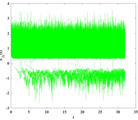
Furthermore, we explore possibility of preserving positivity of the two methods using the

simulation results. The true solution of the SDE (4.1) starting from a positive initial value

will never cross the origin, see Appendix for the proof. It can be seen from the 3000 simulated

paths with the stepsize ∆ = 2−7 _{in Figures 2 and 3 that the partially truncated EM method}

has higher chance to preserve the positivity than the fully tamed method. It should be noted

that the structure of either the partially truncated EM or the fully tamed method would not

guarantee non-negative numerical solutions. Therefore, it would be interesting to conduct

some rigorous analyses on the probability of non-negative solutions of both the two methods.

We have been working on this topic and will report it in the future work.

5

Conclusion

The main contribution of this paper is that we removed a restrictive condition imposed in [3]

Figure 2: The 3000 sample paths generated by the partially truncated EM method.

A couple of examples were used to highlight the advantages of our new results compared with

the earlier ones in [3]. New techniques were developed in this paper to obtain the results.

Appendix

Now we prove almost all the sample path of dx(t) = (x(t)−x5(t))dt+x2(t)dB(t) starting

from a non-zero state, given x(0)>0, will never reach the origin.

Define the stopping time,

τk = inf{t >0 :x(t)∈/[

1

k, k]}.

Clearly, τk is increasing as k → ∞. Set τ∞ = lim

n→∞τk, if we can prove τk

a.s.

−→ ∞ as k → ∞,

then x(t) > 0 a.s. for all t > 0. That is to say, to complete the proof, we need to show

that τ∞ = ∞. To prove this, for any constant T, if P{τk ≤ T} → 0 as k → ∞, then we

have P{τ∞ =∞}= 1, which is the required assertion. For θ ∈ (0,1), define a C2_{− function}

V : (0,∞)→(0,∞) by

V(x) = xθ−1−θlog(x).

It is clear that V(·)≥ 0 and V(x) → ∞ as x→ ∞ or x →0. Applying the Itˆo formula

yields

dV(x(t)) =

(θxθ−1(t)− θ

x(t))(x(t)−x

5_{(t)) +} 1

2(θ(θ−1)x

θ−2_{(t) +} θ

x2_(t))x 4_(t)

dt

+(θxθ−1(t)− θ

x(t))x

2_(t)dB(t)

By boundedness of polynomial, for θ ∈(0,1), there exists a constant K1 such that

θxθ−θxθ+4−θ+θx4+ 1

2θ(θ−1)x

θ+2₊ 1

2θx

2 _≤K

1.

Therefore, for any t∈[0, T],

EV(x(t∧τk))≤V(x(0)) +K1T.

So

P{τk ≤T}

V(1

k)∧V(k)

≤_EV(x(T ∧τk))≤V(x(0)) +K1T.

Then we have P{τk ≤T} →0 since V(_R1)∧V(k)→ ∞ ask → ∞.

That is

Acknowledgements

The authors would like to thank the Natural Science Foundation of Shanghai (14ZR1431300),

Shanghai Pujiang Program (16PJ1408000), the National Natural Science Foundation of China

(11701378), “Chenguang Program” supported by Shanghai Education Development

Founda-tion and Shanghai Municipal EducaFounda-tion Commission (16CG50), the Natural Science Fund of

Shanghai Normal University (SK201603), the EPSRC (EP/K503174/1), the Leverhulme Trust

(RF-2015-385), the Royal Society (Wolfson Research Merit Award WM160014), the Royal

So-ciety and the Newton Fund (NA160317, Royal SoSo-ciety-Newton Advanced Fellowship) and the

Ministry of Education (MOE) of China (MS2014DHDX020), for their financial support.

References

[1] Bahar, A. and Mao, X., Stochastic delay population dynamics, J. Int. Appl. Math.

11(4)(2004), 377–400.

[2] Ginzburg, V. L. and Landau, L. D.,On the theory of superconductivity, Zh. Eksperim. i

teor. Fiz. 20(1950), 1064–1082.

[3] Guo, Q., Liu, W., Mao, X. and Yue, R.,The partially truncated Euler–Maruyama method

and its stability and boundedness, Appl. Numer. Math. 115 (2017), 235–251.

[4] Hutzenthaler, M., Jentzen, A.,Numerical approximations of stochastic differential

equa-tions with non-globally Lipschitz continuous coefficients, Mem. Amer. Math. Soc. 236(2)

(2015) 99 pages.

[5] Khasminskii R.Z. , Stochastic Stability of Differential Equations, Alphen: Sijtjoff and

Noordhoff, 1980. (Translation of the Russian edition, Moscow, Nauka 1969).

[6] Kloeden, P. E. and Platen, E., Numerical Solution of Stochastic Differential Equations,

Springer-Verlog, Berlin, 1992.

[7] Mao, X., Stochastic Differential Equations and Applications, 2nd Edition, Horwood,

Chichester, UK, 2007.

[8] Mao, X.,The truncated Euler–Maruyama method for stochastic differential equations, J.

[9] Mao, X.,Convergence rates of the truncated Euler–Maruyama method for stochastic

dif-ferential equations, J. Comput. Appl. Math. 296 (2016), 362–375.

[10] Mao, X. and Yuan, C., Stochastic Differential Equations with Markovian Switching,

Im-perial College Press, 2006.

[11] Song, M., Hu, L., Mao, X. and Zhang, L., Khasminskii-Type theorems for stochastic

functional differential equations, Discrete Contin. Dyn. Syst. Ser. B 18(6) (2013), 1697–