Effect of time interval variations on RTK derived distances

(1)

Effect of Time Interval Variations on RTK Derived Distances Page 1 of 151

University of Southern Queensland

Faculty of Engineering and Surveying

EFFECT OF TIME INTERVAL VARIATIONS ON RTK

DERIVED DISTANCES

A dissertation submitted by

Mr. Vincent Stanley Bein

In fulfilment of the requirements of

Course ENG4111 & ENG4412 –Research Project

Bachelor of Spatial Science (Hons)

(2)

ABSTRACT

The research problem statement was to determine if the time elapsed between observing

the first and second point when using Real-Time Kinematic (RTK) Global Navigation

Satellite System (GNSS) affected the accuracy and precision of a derived distance

between the two points. In particular, this paper focussed on the Queensland cadastral

system and RTK derived distances which are to be used on cadastral survey plans.

Several days of RTK GNSS (GPS and GLONASS only) data was collected under

laboratory type conditions. Several processing strategies and mathematical models

were developed to work in conjunction with the zero-distance baseline method to

determine distances and produce the results.

The results revealed the one minute data for the latitude distance error at 95% C.I.

achieved ± 4.6mm at the 3 minute window and gradually decreased to ± 7.2mm at the

720 minute window and the longitude distance error achieved ± 4.7mm to ± 8.8mm

respectively. The five second data ranged from ± 6.9mm to ± 8.6mm for latitude at the

95% C.I. from the 3 minute window to the 720 minute window and the longitude

achieved ± 6.4mm to ± 9.0mm respectively.

The five second and one minute data results revealed that there are improvements to

accuracy if points can be observed in quick succession. Waiting a pre-determined time

between observing the same two points does not improve the accuracy of a derived

distance when using a single-base RTK system and the GPS and GLONASS

(3)

Effect of Time Interval Variations on RTK Derived Distances Page 3 of 151 In conclusion, the results achieved in this paper is the first step in determining what

effects time has on RTK results that the practitioner would realise in their real-life field

environment. This first step is vital in not only understanding, the time component of

RTK at the field level but to aid in ensuring all economic benefits are realised in an

ever-demanding environment and to provide the practitioner with necessary confidence

to know the survey being undertaken complies with the survey standards. Further

research using different satellite constellations is required for the profession to realise

some economic benefit. If the practitioner can re-observe the same point while still

(4)

DISCLAIMER

University of Southern Queensland

Faculty of Engineering and Surveying

Limitations of Use

The Council of the University of Southern Queensland, its Faculty of Engineering and Surveying, and the staff of the University of Southern Queensland, do not accept any responsibility for the material associated with or contained in this dissertation.

Persons using all or any part of this dissertation do so at their own risk, and not at the risk of the Council of the University of Southern Queensland, its faculty of Engineering and Surveying or the staff of the University of Southern Queensland. The sole purpose of the unit entitled “Project” is to contribute to the overall education process designed to assist the graduate enter the workforce at a level appropriate to the award.

The project dissertation is the report at of an educational exercise and the document, associated hardware, drawings, and other appendices or parts of the project should not be used for any other purpose. If they are so used, it is entirely at the risk of the user.

(5)

CERTIFICATION

I certify that the ideas, designs and exp

e

_{rimental work, results, analysis and}

conclusions set out in this dissertation are entirely my own efforts, except where otherwise indicated and acknowledged.

I further certify that the work is original and has not been previously submitted for assessment in any other course or institution, except where specifically stated.

Vincent Stanley Bein

Student Number: 0031010799

……….

(Signature)

(6)

ACKNOWLEDGEMENTS

This research was carried out under the principal supervision of Associate Professor Peter Gibbings. I would like to express my sincere gratitude to Professor Gibbings who has provided me with guidance, encouragement and has always kept my spirits up all through my candidature at the University of Southern Queensland.

Appreciation and thanks is also due to Mr Garry Cislowski – Department of Natural resources and Mines for all his support, patience and ongoing encouragement.

(7)

TABLE OF CONTENTS

ABSTRACT ... 2

DISCLAIMER ... 4

CERTIFICATION ... 5

ACKNOWLEDGEMENTS ... 6

TABLE OF CONTENTS ... 7

TABLE OF FIGURES ... 10

LIST OF TABLES ... 13

NOMENCLATURE AND ACRONYMS ... 14

CHAPTER ONE - INTRODUCTION ... 15

1.1PROBLEM STATEMENT ... 21

1.1.1 RTK Accuracy and Precision ... 23

1.1.2 Point Positioning ... 25

1.1.3 Precise Point Positioning ... 26

1.1.4 Temporal and Spatial Error Sources ... 27

1.1.5 Sky view, Obstructions and their Effects ... 28

1.1.6 Queensland Survey Standards ... 30

1.1.7 The Problem ... 31

1.2RESEARCH AIM... 32

1.3JUSTIFICATION ... 32

1.3.1 Motivation ... 34

1.4RESEARCH METHOD ... 35

1.4.1 The Solution ... 35

1.5SCOPE AND LIMITATIONS OF THE RESEARCH PROJECT ... 36

1.6SUMMARY ... 37

CHAPTER 2 – LITERATURE REVIEW ... 38

2.1INTRODUCTION. ... 38

2.2RTKGPS/GNSS... 39

2.3QUEENSLAND SURVEY STANDARDS AND GUIDELINES ... 41

2.4CALIBRATION OF GPS/GNSS... 44

2.5ZERO-BASELINES AND ZERO-DISTANCE BASELINES ... 46

2.5.1 Previous Zero-baseline Method Research ... 46

2.5.2 Zero Baseline... 48

2.5.3 Zero-Distance Baseline... 50

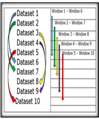
2.6AVERAGING AND TIME INTERVAL (VARIATIONS)WINDOWS ... 54

2.6.1 Averaging ... 56

2.6.2 Windowing ... 57

2.5CONCLUSIONS ... 60

CHAPTER 3 ... 62

METHODOLOGY ... 62

3.1INTRODUCTION ... 62

3.2SITE SELECTION ... 63

3.3BASE STATION,RTKGNSSRECEIVER AND RADIO DETAILS ... 64

3.3.1 Testing Site ... 65

3.3.2 Base Receiver Information Details: ... 65

3.3.3 Trimble RTK GNSS Receiver Details: ... 66

3.4SITE SPECIFICS ... 68

3.4.1 Equipment Validation ... 71

3.4.2 Ancillary Equipment ... 72

3.5USING ZERO-DISTANCE BASELINE TESTING METHOD ... 73

3.6DATA COLLECTION VERIFICATION PROCESS ... 73

(8)

3.6.2 Data Evaluation/Integrity ... 76

3.6.3 Data Processing ... 76

3.6.4 Processing Strategy ... 77

3.6.4.1 Single Epoch Processing Strategy ... 77

3.6.5.2 Five Second Averaged Single Epochs of Collected Data ... 78

3.6.5.3 One Minute Averaged Single Epochs of Collected Data ... 78

3.6.5.4 Tiers of Processing Strategy ... 79

3.6.6 Validation Method of Computations ... 81

3.7CONCLUSION OF CHAPTER 3 ... 84

CHAPTER 4 ... 86

4.1INTRODUCTION ... 86

4.1.1 Data Validation ... 87

4.1.2 Single Epoch Data Analysis ... 93

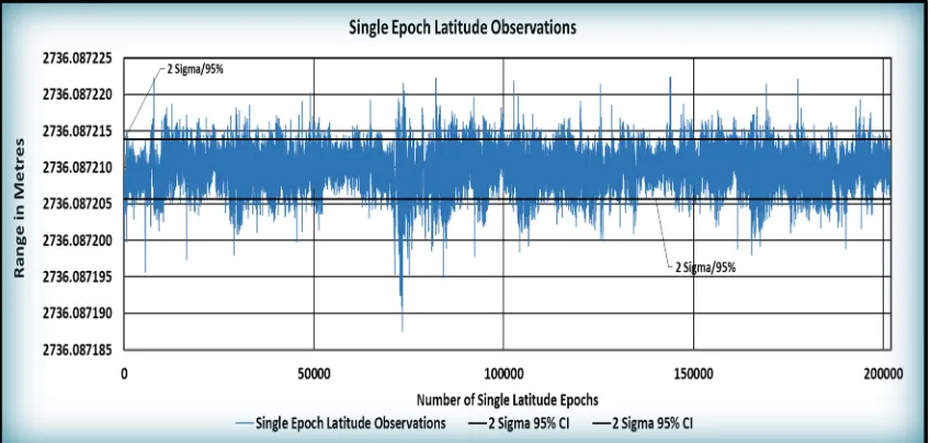
4.1.3 Single Latitude Epochs Defined ... 97

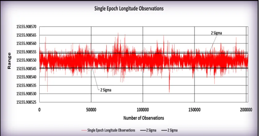
4.1.4 Single Longitude Epoch Defined ... 99

4.1.5 Notes ... 100

4.2FIVE SECOND/THREE MINUTE WINDOW DATASET AT 95%CONFIDENCE INTERVAL ... 100

4.3FIVE SECOND OBSERVATION TIME WITH INCREASING WINDOWS AT 95%CONFIDENCE INTERVAL ... 105

4.4FIVE SECOND OBSERVATION TIME AT THE THIRTY MINUTE WINDOW ... 108

4.5FIVE SECOND/NINETY-FIFTH PERCENTILES ... 111

4.5.1 Five Second/Ninety-fifth (95th_{) Percentile Distances ... 111}

4.5.2 Region at which 95th_{Percentile of Five Second Data Falls ... 112}

4.6ONE MINUTE OBSERVATION TIME DATASET ... 113

4.6.1 One Minute – with Thirty Minute Window Point Positions at 95% C.I. ... 114

4.6.2 One Minute Dataset – Maximum and the 95th_{Percentile Distances ... 115}

4.6.3 Region at which the Ninety-fifth Percentile of One Minute Data Falls ... 117

4.7ONE MINUTE OBSERVATION TIME WITH INCREASING WINDOWS AT 95%CONFIDENCE INTERVAL... 118

4.8FIVE SECOND AND ONE MINUTE OBSERVATION OVER INCREASING WINDOWS AT 95%CONFIDENCE INTERVAL .... 120

4.9SUMMARY ... 121

CHAPTER 5 ... 122

RESULTS AND DISCUSSION ... 122

5.2DISCUSSION ... 122

5.3RESULTS ... 124

5.3.1 Single Epoch Data Analysis ... 124

5.3.2 Single Latitude Epochs Defined ... 124

5.3.3 Single Longitude Epochs Defined ... 124

5.3.4 Five Second/Three Minute Window Point Positions at 95% Confidence Interval... 125

5.3.5 Five Second Observation Time with Increasing Windows at the 95% Confidence Intervals ... 126

5.3.6 Five Second Observation Time at the Thirty Minute Window ... 127

5.3.7 Five Second/95th_{Percentiles ... 128}

5.4ONE MINUTE OBSERVATION TIME DATASET ... 128

5.4.1 One Minute Dataset Point Positions with increasing Windows at the 95% Confidence Interval ... 128

5.4.2 One Minute – with Thirty Minute Window Point Positions at 95% C.I. ... 129

5.4.3 One Minute Dataset – Maximum and the 95th_{Percentile Distances ... 130}

5.4.4 One Minute Observation Time with Increasing Windows at 95% Confidence Interval ... 134

5.5FIVE SECOND AND ONE MINUTE OBSERVATIONS OVER INCREASING WINDOWS AT THE 95%CONFIDENCE INTERVAL ... 135

5.6SUMMARY ... 136

5.7IMPLICATIONS ... 137

CHAPTER 6 ... 138

CONCLUSION ... 138

6.2MEETING THE AIMS AND OBJECTIVES ... 138

6.3FINDINGS AND RECOMMENDATIONS... 139

6.4COMPLIANCE TO STANDARDS ... 139

6.5OBSERVATION TIMES ... 140

6.6TIME WINDOWS ... 140

(9)

6.8RECOMMENDATIONS ... 144

6.9CONCLUSION AND PROJECT CLOSURE ... 145

REFERENCES ... 146

(10)

TABLE OF FIGURES

FIGURE 1: RADIAL SURVEY TECHNIQUE ... 23

FIGURE 2: RTK OBSERVATION TECHNIQUE ... 24

FIGURE 3: ERRORS ... 28

FIGURE 4: SIGNAL OBSCURATION ... 29

FIGURE 5: RTK DERIVED DISTANCE ... 31

FIGURE 6: RTK RADIAL SURVEY ... 34

FIGURE 7: SPLITTER FOR ZERO-BASELINE SETUP ... 48

FIGURE 8: SPLITTER AND GEODETIC ANTENNA SETUP ... 49

FIGURE 9: SIMULTANEOUS TRIGGERING OF BOTH VRS & RTK ... 49

FIGURE 10: USQ TRIMBLE ZEPHYR MODEL 2 ANTENNAE ... 50

FIGURE 11: ZERO-DISTANCE ERROR WITH BEARING ERROR INCLUDED ... 51

FIGURE 12: TRUE ZERO-DISTANCE BASELINE... 52

FIGURE 13: AVERAGING FIGURE 14: WINDOWING ... 57

FIGURE 15: ACCURACY DEFINITIONS ... 59

FIGURE 16: RINGS OF ACCURACY FOR GPS ... 59

FIGURE 17: POSITION ACCURACY MEASURES ... 59

FIGURE 18: USQ CORS BASE STATION 'ANANGA' ... 63

FIGURE 19: 'ANANGA' CORS PSM ... 64

FIGURE 20: SKY VIEW & STAY WIRES ... 65

FIGURE 21: LIGHTNING RODS ... 66

FIGURE 22: TRIMBLE R8-3 RTK GNSS RECEIVER ... 67

FIGURE 23: USQ RTK GNSS GEODETIC ANTENNA ... 67

(11)

FIGURE 25: RE-BROADCASTER USQ Z-BLOCK Z120 ... 69

FIGURE 26: ANTENNA PHASE CENTRE ... 70

FIGURE 27: TRIMBLE ZEPHYR GEODETIC MODEL 2 ANTENNA ... 71

FIGURE 28: ANTENNA MEASUREMENT ... 71

FIGURE 29: USQ 450 TDL RADIO ... 72

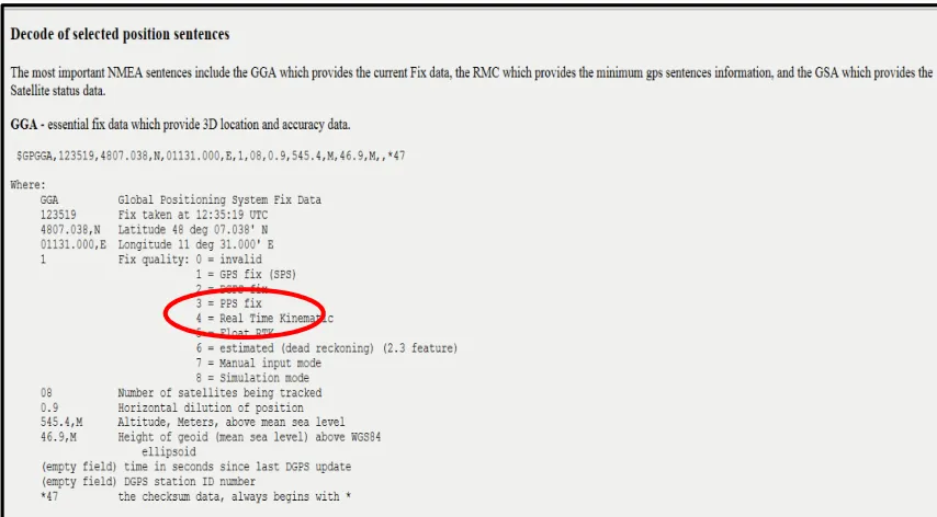
FIGURE 30: NMEA-0183, GGA FIELD CODE ... 75

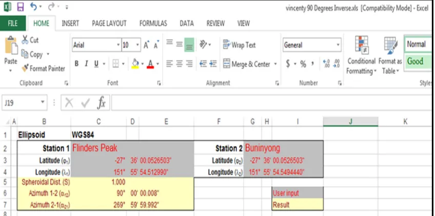
FIGURE 31: 90 DEGREES/1.0M INVERSE SOLUTION... 82

FIGURE 32: 90 DEGREES/1.0M DIRECT SOLUTION ... 82

FIGURE 33: 90 DEGREES/1.0M EXCEL LONGITUDE CHECK ... 82

FIGURE 34: ZERO DEGREES/1.0M DIRECT SOLUTION ... 83

FIGURE 35: ZERO DEGREES/1.0M INVERSE SOLUTION ... 83

FIGURE 36: EXCEL FORMULAE LATITUDE CHECK ... 83

FIGURE 37: 6KM TO 22KM AT 68% ... 88

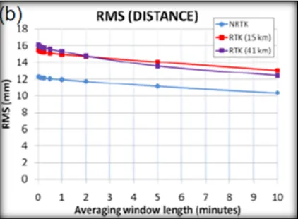
FIGURE 38: 15KM TO 41KM AT 68% ... 90

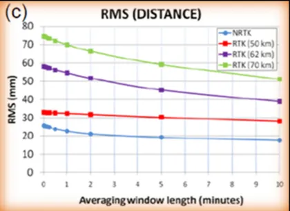
FIGURE 39: 50KM TO 70 AT 68% ... 91

FIGURE 40: LATITUDE POINT POSITION RANGE WITH 95% C.I. OF DATASET INCLUDED. ... 96

FIGURE 41: LONGITUDE POINT POSITION RANGE WITH 95% C.I. OF THE DATASET ... 97

FIGURE 42: SINGLE EPOCH LATITUDE POINT POSITION HISTOGRAM ... 97

FIGURE 43: SINGLE EPOCH LATITUDE POINT POSITION DESCRIPTIVE STATISTICS ... 98

FIGURE 44: SINGLE EPOCH LONGITUDE POINT POSITION HISTOGRAM ... 99

FIGURE 45: SINGLE EPOCH LONGITUDE POINT POSITION DESCRIPTIVE STATISTICS ... 99

FIGURE 46: WINDOWING EFFECT ... 101

FIGURE 47: 5 SECOND/3 MINUTE LONGITUDE DISTANCE ERRORS WITH 95% C.I. ... 102

FIGURE 48: 5 SECOND/3 MINUTE LATITUDE DISTANCE ERRORS WITH 95% C.I. ... 103

(12)

FIGURE 50 : 5 SECOND/3 MINUTE LONGITUDE DISTANCE HISTOGRAM ... 104

FIGURE 51: PICTORIAL OF THE 5 SECOND AVERAGED EPOCH PRECISIONS OVER INCREASING TIME WINDOWS AT 95% C.I. ... 105

FIGURE 52: RE-GRAPHED 5 SECOND DATASET OVER INCREASING WINDOWS AT 95% C.I. ... 106

FIGURE 53: 5 SECOND/30 MINUTE WINDOW DISTRIBUTION HISTOGRAM ... 108

FIGURE 54: LONGITUDE - 5 SECOND/30 MINUTE WINDOW DISTRIBUTION HISTOGRAM ... 108

FIGURE 55: LATITUDE 5 SECOND/30 MINUTE WINDOW DISTANCES ... 109

FIGURE 56: LONGITUDE 5 SECOND/30 MINUTE WINDOW DISTANCES ... 109

FIGURE 57: 95TH PERCENTILE - ABSOLUTE MEASURED DISTANCE AT INCREASING WINDOWS ... 111

FIGURE 58: 95TH PERCENTILES – THE VALUE AT WHICH 95% OF DATA FALLS BELOW ... 112

FIGURE 59: RE-GRAPHED FIGURE 58 - 3 MINUTE TO 90 MINUTE WINDOWS ... 112

FIGURE 60: 1 MINUTE DATASET POINT POSITIONS AT INCREASING WINDOWS AT 95% C.I. ... 113

FIGURE 61: 1 MINUTE/30 MINUTE WINDOW LATITUDE AND LONGITUDE POINT POSITIONS WITH THE 95% CONFIDENCE INTERVALS ... 115

FIGURE 62: 95TH PERCENTILES - DISTANCES AND MAXIMUM DISTANCES ... 116

FIGURE 63: 1 MINUTE/95TH PERCENTILE LATITUDE & LONGITUDE - 3M TO 720M WINDOWS ... 117

FIGURE 64: 1 MINUTE DATASET - PRECISION AT 95% C.I. AS A FUNCTION OF TIME ... 118

FIGURE 65: DISTANCE ERROR AS A FUNCTION OF TIME ... 128

FIGURE 66: 1 MINUTE/30 MINUTE POINT POSITIONS ... 130

FIGURE 67: 1 MINUTE 95TH PERCENTILE DISTANCES OVERLAID WITH THE 95% C.I. ... 131

FIGURE 68: 1 MINUTE - 95TH PERCENTILE & MAXIMUM DISTANCES WITH THE 95% C.I. ... 132

FIGURE 69: NRTK VS RTK: DISTANCE DEVIATIONS FROM THE MEAN ... 133

FIGURE 70: 1 MINUTE/INCREASING WINDOWS - LATITUDE AND LONGITUDE 95% C.I. DISTANCE ERROR OVERLAIN WITH CSR VECTOR ACCURACY ... 134

(13)

LIST OF TABLES

TABLE 1: 95% CONFIDENCE INTERVAL OF 201848 SINGLE EPOCHS OF COLLECTED DATA ... 92

TABLE 2: RANGE OF SINGLE EPOCH LATITUDE AND LONGITUDE POINT POSITIONS ... 94

TABLE 3: LATITUDE AND LONGITUDE SINGLE-EPOCH 95% CONFIDENCE INTERVAL OF THE POINT POSITIONS. ... 95

TABLE 4: RHO & NU CORRECTED FOR HEIGHT AT THAT POINT ... 95

TABLE 5: SINGLE EPOCH POINT POSITION COLLECTED DATA MEAN/MEDIAN/MODE DIFFERENCES. ... 100

TABLE 6: DESCRIPTIVE STATISTICS FOR 5 SECOND/3 MINUTE WINDOW DATASET ... 102

TABLE 7: TABULAR DESCRIPTION OF THE 5 SECOND DATASET OVER INCREASING TIME WINDOWS AT 95% C.I. ... 106

TABLE 8: RANGE OF 5 SECOND DATASET AT INCREASING WINDOWS ... 107

TABLE 9: 5 SECOND/30 MINUTE WINDOW STATISTICS ... 110

TABLE 10: 5 SECOND/95TH PERCENTILE AND MAXIMUM DISTANCES ... 111

TABLE 11: 5 SECOND - 95TH PERCENTILES AT INCREASING WINDOWS ... 113

TABLE 12: 1 MINUTE DATASET POINT POSITIONS AT INCREASING WINDOWS AT 95% C.I. ... 114

TABLE 13: 1 MINUTE/30 MINUTE LATITUDE AND LONGITUDE POINT POSITIONS WITH THE 95% C.I. 115 TABLE 14: 1 MINUTE DATASET WITH INCREASING WINDOWS - 95TH PERCENTILE DISTANCES... 116

TABLE 15: 1 MINUTE - 95TH PERCENTILE LATITUDE & LONGITUDE - 3M TO 720M WINDOWS ... 117

TABLE 16: 1 MINUTE DATASET AT INCREASING WINDOWS AT 95% C.I. ... 119

TABLE 17: 1 MINUTE & 5 SECOND DATASETS AT INCREASING WINDOWS AT 95% C.I. ... 120

TABLE 18: 1 MINUTE DATASET AT INCREASING WINDOWS AT 95% C.I. ... 129

TABLE 19: 1 MINUTE/30 MINUTE POINT POSITIONS ... 130

(14)

NOMENCLATURE AND ACRONYMS

The following abbreviations have been used throughout the text and references:-

APC Antenna Phase Centre

CI Confidence Interval

CQ Coordinate Quality

CORS Continuously Operating Reference Station

CSR Cadastral Survey requirements

DOP Dilution of Precision

DoD Department of Defence in America

EDM Electronic Distance Measurement

GNSS Global Navigation Satellite System

GPS Global Positioning System

ICSM Intergovernmental Committee on Surveying and Mapping

MGA Map Grid of Australia

PPP Precise Point Positioning

ppm parts per million

PSM Permanent Survey Mark

RTK Real-time Kinematic

SBQ Surveyors Board of Queensland

SIS Signal-in-Space

SMI Act Surveying and Mapping Infrastructure Act 2003

SPS Standard Positioning Service

SP1 Special Publication #1

SV Space Vehicle

(15)

CHAPTER ONE - INTRODUCTION

There are several grades of Global Navigation Satellite Systems (GNSS) instruments

and systems available to suit all needs. The systems are defined by their positional

accuracy capabilities. The can be further defined as civilian, mapping, surveying and

military grade. The most basic GNSS point positioning system is used for recreational

purposes such as orienteering, fishing, boating and the in-car navigation system. The

quality of information coming out of a GNSS is dependent on the quality of the

information going in and the quality of the information has a cost associated to it. The

more accurate and precise the more expensive. Real-Time Kinematic (RTK) is a survey

grade technique which utilises the signal from GNSS to obtain a point position in real

time.

RTK, like all surveying systems, does have accuracy and precision limitations which are

caused by systematic errors that occur prior to the receiver accepting the broadcast

navigation signal. RTK’s introduction into Australia prompted regulatory agencies to

update the existing survey standards and guidelines. These standards and guidelines

have been dynamic, based on substantiated quality research and reflect the technological

changes and developments as they occurred or became apparent. These

accomplishments have prompted the requirement for more research. Recent times has

seen more research on the temporal characteristics of using the RTK technique to derive

distances between separate observations.

These derived distances are used for many applications such as; pegging land allotments

and displaying ground distances on survey plans, engineering setout works and civil

(16)

Effect of Time Interval Variations on RTK Derived Distances Page 16 of 151 distances is paramount. In some instances, considerable time can elapse before a

practitioner can observe the second point which is needed to derive (compute) a

distance between two points. This time interval could be as short as three or four

minutes or as long as hours and even days at times. The effect of time interval variation

when using RTK to derive a distance demands further research to assess if any changes

occur to the normal RTK error budget.

With due regard to other applications and professions, the importance of an accurate

cadastre and State Database is also paramount when considering the importance of land

to the economy. The intent of this dissertation is to develop a workable mathematical

model to extrapolate distances from the collected data and determine the maximum,

minimum, range, standard deviation and ninety-five percent (95%) confidence interval

of pre-determined averaged datasets and increasing time interval windows. As

appropriately mentioned in the previous sentence this research project is about derived

distances between points at either end of a line when using an RTK single-base system.

Put into a simple context, the zero-distance baseline accepts that the RTK observations

are random and the distances are calculated between the observations as they ‘wander’

around. To elaborate, if we observe a position now, we achieve a set of coordinates

(say -26⁰ 30’ 00”, 150⁰ 30’ 00”) computed by the data recorder setup parameters e.g.

average of 5 epochs. We wait 30 minutes and re-observe the same point and achieve

coordinates of say, -26⁰ 30’ 30” & 150⁰ 30’ 30”. The difference between these two

coordinates is the zero-distance baseline (a distance expressed in metres in a one

dimensional form – latitude and longitude) and, obviously, because of the temporal and

spatial errors associated with RTK the coordinates of the same point ‘wander’ around

(17)

Effect of Time Interval Variations on RTK Derived Distances Page 17 of 151 error budget and concentrates more on how the practitioner can work with it. No one

observation is accepted as the true value for a point. It does not compute a mean of the

sample.

Initially, to set a benchmark, the single epochs of latitude and longitude will be

statistically analysed and graphed to ascertain trends, behaviours and patterns.

Following, the mathematical model will derive the arithmetic mean of the 201848 single

epochs of collected data. Next, the entire dataset will be divided into the predetermined

sets of averaged epochs of data of five second and one minute sets. These averaged

epochs of data will be called datasets and will represent observation time on the point

and are designed to replicate how long the practitioner might feasibly spend observing a

point. The five second average was chosen to set a platform which is well below any

recommended time span by notable researchers (Edwards et al. 2010; Gibbings & Zahl

2014a; Janssen & Haasdyk 2011b) and below the minimum recommended time in the

latest Queensland Cadastral Survey Requirements (Spatial Policy of Department of

Natural Resources and Mines. Cadastral Survey Requirements 2015, Version 7.0). The one minute observation was chosen to allow for comparisons with the single epochs of

latitude and longitude, the five second platform and a combination of all when

appropriate.

The time interval variation, from this point forward called a time interval window or

simply a window, sampling rate will commence at three minutes. The rate will then be

increased to five (5) minutes (m), 10m, 15m, 20m, 25m, 30m, 60m, 120m, 240m, and

(18)

Effect of Time Interval Variations on RTK Derived Distances Page 18 of 151 The time interval of 720m or twelve hours is to ensure the twelve hour orbit cycle of the

Space Vehicles (SV) is accounted for and the many multiple variations of satellite

configurations are experienced. Next, whilst holding the first window of five (5)

seconds the maximum, minimum, range, standard deviation and the ninety-five percent

(95%) confidence interval (C.I.) will be calculated for the entire time interval sampling

windows/increments. The 5 second dataset will undergo a single analysis and

subsequent graphing, involving increasing the time window to ascertain what effect

time windows has on precision.

The 5 second and 1 minute datasets will be analysed and graphed together at increasing

time windows and compared with the single epoch analysis and against one another as

appropriate. This mathematical process will be rigorous for all windows and the results

graphed against an absolute zero-distance baseline. The zero-distance baseline

produces distances relative to the true value coordinates and are expressed in metres.

All residual distance errors will be expressed in metres as latitude and longitude

separately and respectively and graphed accordingly.

Every instrument has intrinsic uncertainty when measuring the same point multiple

times and this uncertainty is usually stated as a constant and a distance dependent parts

per million (ppm) error. The RTK error is expressed in this same manner but its

accuracy and precision has a pattern and at the same time a randomness that is caused

by several temporal errors. The ever-changing satellite configuration, timing errors and

the lack of a yet-to-be discovered suitable model that addresses the atmospheric and

tropospheric conditions that broadcast ephemeris must travel through are some of the

(19)

Effect of Time Interval Variations on RTK Derived Distances Page 19 of 151 These errors, which are uncontrollable by human intervention, change as time expires

and the multitude of factors that affect these errors are inconsistent in themselves. The

significance of this phenomenon must be understood so the mathematical model is

designed to extract the necessary statistical data to be evaluated. Each epoch of data is a

random variable in itself and each windowed dataset will be a random variable in itself

also.

Each satellite has its own inherent errors and to overcome this the software inside the

receiver has a specifically designed set of satellite selection algorithms. These

algorithms allows the software to select a number of the most suitable satellites which

have the lowest Dilution of Precision (DOP) values (Langley 1999). DOP is, basically,

a measure of the number of visible satellites and their three dimensional position. The

lower the DOP the better the estimate of the position to its true value. The minimum

number of satellites required to obtain a resolution is four. One to solve for each of the

four unknowns; x, y, z and time.

It is common to measure the quality of the results by determining the mean but

precision determines the repeatability. As the dataset is windowed it is expected that

random variability will become somewhat hidden or disguised and it is also envisaged

the range established by averaging the entire dataset will remain constant. On

derivation of the results from the mathematical model comparisons will be made to the

(20)

Effect of Time Interval Variations on RTK Derived Distances Page 20 of 151 In Queensland, the Department of Natural Resources and Mines (DNRM) and the

Surveyors Board of Queensland (SBQ) are the primary regulatory authorities. Global

Satellite System (GPS) were introduced into Australia in 1994 and the main surveying

manuals for surveyors was the Surveyors Operational Manual (SOM) and the Board

Operational Manual (BOM). Like any new technologies ‘teething problems’ can be

experienced and as time expired RTK presented its own challenges.

Some of these challenges presented themselves in late 2012, when the Surveyors Board

of Queensland recognised there were some issues and potential confusion amongst

practitioners regarding the use of RTK for cadastral surveying. This prompted the SBQ

to release a guideline (Surveyors Board of Queensland November, 2012) which

provided clarification on the identified issues. Since then Gibbings, P. & Zahl, M.

(2014b) have released two articles with the express intention of emphasising the specific

capabilities and limitations of RTK. Gibbings, P. & Zahl, M. (2014b) made

comparisons between the results of their testing and the current Queensland cadastral

surveying legislation, survey standards and recommended guidelines.

The Surveying and Mapping Infrastructure Act 2003 (SMI Act) and the Surveyors Act

2003 provides legislative support to the Department of Natural Resources and Mines

(DNRM) and the SBQ. The Cadastral Survey Standards (CSR) is a standard under of

the Surveying and Mapping Infrastructure Act 1994 (SMI Act) and Section 3.4.2

(Measurement Accuracy) of the CSR (commonly known as Survey Standards) provides

several determinations as to how the accuracy of a cadastral survey in terms of both

angular and linear misclose can be achieved. DNRM has recently released version 7.0

(21)

Effect of Time Interval Variations on RTK Derived Distances Page 21 of 151 Version 7.0 of the CSR includes an entire chapter on the use of Global Navigation

Satellite Systems (GNSS) for cadastral surveying in Queensland. This new version

does provide much needed clarification on the issues identified by the SBQ but it is not

completely exhaustive. Previous research by Gibbings and Zahl (2014) has already

provided sufficient support for these new changes but it, also produced more questions

and the need for more research to further advance the understanding of RTK.

Therefore, it is a prerequisite and a professional obligation on spatial science students

and professionals to continue expanding on the existing research. This is especially

correct given the new SBQ guideline (2012), the release of the new CSR’s and the

increased pressure on practitioners to comply with relevant standards.

1.1 Problem Statement

Does the time elapsed between observing the first point and second point when using

RTK GNSS, affect the accuracy and precision of the derived distance between the two

points? This elapsed time will be referred to the ‘time interval variation or time interval

window or window’ from this point forward. No measuring instrument can measure a

distance perfectly and RTK GNSS is no exception. This imperfection is often referred

to as an error budget or biases’. The error budget consists of random, systematic and

gross errors. It is well-known and proven that the errors that influence the final RTK

positions have the potential to create survey standard compliance issues for the survey

profession, especially, when the survey standards appear more stringent than the known

limitations and capabilities of an RTK system (Gibbings & Zahl 2014b; Higgins 2001).

However, there has been little research on what effects time interval variations has on

RTK derived distances. That is, does the time elapsed between observing the first point

(22)

Effect of Time Interval Variations on RTK Derived Distances Page 22 of 151 Conventional surveying instruments, sometimes referred to as Terrestrial Instruments

(TI), Electromagnetic Distance Measurement Equipment (EDME) or a Total Station

(TS), are not affected by the errors associated with RTK. However, TI’s, TS’s and

EDME’s can be affected by other more localised issues such as the local climatic

conditions. The local meteorological data is entered into them and the survey

commences and is, generally, completed within the manufacturers’ instrument

specifications provided the obligatory check and balances are in place. TI’s, if

standardised correctly, are capable of consistently measuring the same distance to the

same level of accuracy and precision between the same two points, as per the individual

instrument manufacturer’s specifications, day after day. The same level of accuracy and

precision mentioned in this context satisfies the current Queensland survey standards.

RTK does not have this ability.

In fact, RTK surveys are radial in nature and distances between two points being

observed is calculated and not measured. In addition to this, due to its inherent errors, it

is extremely difficult for RTK to achieve or repeat the same computed distance or level

of accuracy and precision between the same two observed points after multiple

attempts. However, RTK’s main advantages are its ability to measure longer distances

which negates the need for multiple setups and it is not subject to intervisibility issues

(23)

1.1.1 RTK Accuracy and Precision

Many researchers have, since the inception of GPS, established the accuracy and

precision for point positioning using RTK and the subsequent effects to a distance on a

calculated line (Gibbings & Zahl 2014b). ‘Calculated or derived’ meaning not

measured because RTK surveys are radial in nature. However, to the authors’

knowledge, little research exists which describes what the effects are to an RTK derived

distance as the time between observing the first and second point increases. As seen in

Figure 1, the RTK surveying technique is similar to undertaking a topographic survey

with a conventional survey instrument.

Figure 1: Radial Survey Technique

Source: http://www.slideshare.net/xuhui6996/em-1110-11005-control-and-topographic-surveying.

An RTK receiver uses the carrier phase and code observables to define its position and

the accuracy and precision of its point is estimated because orbital errors, satellite clock

errors, multipath and atmospheric errors (Olynik 2002) are predicted. These errors can

be well managed and to some extent reduced by adopting suitable techniques (Higgins

2001; Spatial Policy of Department of Natural Resources and Mines 2010-Version 6.0,

(24)

Effect of Time Interval Variations on RTK Derived Distances Page 24 of 151 The correct management of these errors can improve the positional and local uncertainty

(Inter-Governmental Committee on Surveying and Mapping (ICSM) October 2014) of

its point.

RTK is a passive system unlike conventional surveying instruments which receive a

return signal. This gives the conventional instrument an advantage because it sends and

receives multiple signals, as defined by the operator, which in itself has some

‘redundancy’ effect. An RTK system receives a data signal continuously, as seen in

Figure 2, and this signal contains errors outside the control of the user. Attached to this

signal is the broadcast ephemeris. The broadcast ephemeris contains predications on

where the satellite (spatial position), commonly called a space vehicle (SV), should be

and not where it truly is. This is defined as orbital errors and each SV has its own

prediction errors. It is not until the SV has passed a point before its true spatial position

can be accurately determined and, therefore, defining the rover receiver’s more

accurately. The main advantage of RTK would be lost if post processing of data is

required.

Figure 2: RTK Observation Technique

(25)

Effect of Time Interval Variations on RTK Derived Distances Page 25 of 151 The instrument collecting the data, commonly called a data collector, has built in

mathematical statistical algorithm’s which, based on the parameters and definitions set

by the user, accepts a predetermined number of epochs of data and mathematically

obtains the most probable value (MPV) for the point position. While this process

appears to isolate and neglect the errors previously mentioned it only reduces the

likelihood of accepting outliers by the use of simple statistics.

Outliers still exist and, initially, the user must rely on confidence, baseline accuracies

and Root Mean Square (RMS) values (highlighted on the status line on the data

recorder) before accepting the coordinates of the point. Whilst the magnitude or

randomness of these errors are not immediately noticeable there are appropriate survey

techniques available which are used to reveal them.

1.1.2 Point Positioning

Most new vehicles today come equipped with an in-car navigation system and a

recreational handheld GPS can be purchased for a few hundred dollars. There is no

special GPS receiver signals associated with the different grades of GPS instead the

internal software of individual grade GPS receivers have different capabilities for

extracting relevant information from the signals to achieve certain levels of accuracy

and precision. Obviously, purchase prices vary accordingly.

In short, recreational and professional GPS units are designed and built for different

purposes. As a general rule, recreational GPS’s have a positional accuracy of ±10m,

(26)

1.1.3 Precise Point Positioning

In the 1990’s, the Jet Propulsion Laboratory at the National Aeronautical Space Agency

(NASA) in America pioneered new techniques that did not require differencing to

obtain precise positions. They labelled it Precise Point Positioning (PPP) (Nistor. S &

A.S. 2012). The word ‘Precise’ is used in the description to differentiate it from relative

point positioning. PPP is different from RTK. RTK requires two receivers, one base

receiver and one rover receiver whereas PPP requires a rover receiver only. PPP

receives differential corrections via kinematic or static mode and relies on predicted

satellite orbits, ionospheric models and real time satellite estimates (van Bree &

Tiberius 2012) to establish its position. Basically, PPP’s point position uses a GNSS

code observable and the navigation message. The accuracy and precision of PPP is

generally greater than RTK (van Bree & Tiberius 2012).

Research and testing by van Bree & Tiberius (2012) achieved standard deviations of

0.15 and 0.30m for the horizontal and vertical coordinates, respectively, with 95% error

values of approximately 0.30m and 0.65m. PPP is available through commercial

service providers for a fee and only a single GNSS receiver is needed which suggests

the cost of the fee is offset by the lack for the need for a base receiver.

PPP has lower positional accuracy than RTK which makes it unsuitable for cadastral

surveying in Queensland. PPP also requires longer convergence times, is not

constrained by baseline length and presents an efficient alternative for applications such

(27)

1.1.4 Temporal and Spatial Error Sources

The American Department of Defence (DoD) established the conventional GPS system

for military purposes and maintains full control and authority with the system. The

following passage taken from Section 2.4.5 (Excluded Errors) of the ‘Global positioning system standard positioning service performance standard’ (DoD 2001) page 15, provides clear and definitive evidence of the errors associated with GNSS

systems (refer Figure 4). Note dot points with the following superscripts 1, 2, 3, 4, 6

and 7 are not controllable by any human source and can occur randomly but are always

present and have a direct influence on the final position (refer to Figure 3).

“The performance standards in Section 3 of this SPS PS do not take into consideration

any error source that is not under direct control of the Space Segment or Control

Segment. Specifically excluded errors include those due to the effects of:

• Signal distortions caused by ionospheric and/or tropospheric scintillation1

• Residual receiver ionospheric delay compensation errors2

• Residual receiver tropospheric delay compensation errors3

• Receiver noise (including received signal power and interference power) and

resolution4

• Receiver hardware/software faults5

• Multipath and receiver multipath mitigation6

• User antenna effects7

(28)

Effect of Time Interval Variations on RTK Derived Distances Page 28 of 151 A substantial amount of research has established the spatially and temporally correlated

errors (El-Rabbany & Kleusberg 2003; Olynik 2002) which affects the accuracy and

precision of RTK. Spatially correlated errors occur when the magnitude of the error is

similar at two different locations and errors are temporally correlated when their

magnitude is similar over a period of time (Miller, O'Keefe & Gao 2012).

Figure 3: Errors

Source: http://forum.xda-developers.com/showthread.php?t=1697306.

1.1.5 Sky view, Obstructions and their Effects

Dilution of Precision (DOP), in GPS positioning, is an indication of the geometric

strength of the configuration of the satellites in a particular constellation at a particular

moment and hence the quality of the results that can be expected (Van Sickle 2011).

The following statement taken from Section B.4.3 of the ‘Global positioning system standard positioning service performance standard’ (DoD 2001) page B38 and the following supporting figure 1, provide an explanation on how the Dilution of Precision

(29)

Even when there is only one nearby obstruction that only blocks one SPS (Standard

Positioning Service) SIS (Signal-In-Space), the loss of that SPS SIS can radically

alter the DOP values. In such obstacle-rich environments, it is difficult to try to

predict in advance which satellite's SPS SIS will be blocked and when that blockage

will start or end (DoD 2001).

Figure 4: Signal Obscuration

Sourced: http://www.navcen.uscg.gov/pdf/gps/geninfo/2001SPSPerformanceStandardFINAL.pdf

The above-mentioned comment and Figure 4 relates specifically to the use of RTK in an

American urban environment. However, the paradigm is applicable to all world

locations and environment. A close inspection of Figure 4 reveals the minimum

elevation mask is 9º which is not a recommended standard under the current

Queensland Cadastral Survey Requirements. Figure 4 does highlight the effect

obscuration can have on RTK results especially if it being used where obstructions do

(30)

1.1.6 Queensland Survey Standards

Section 3.4.2 (Measurement Accuracy) of the Cadastral Survey Requirements (CSR),

Version 7.0, states the accuracy of a cadastral survey in terms of both angular and linear

misclose, and then goes on to add the requirement that, ‘All surveyed lines (e.g. boundary lines, connections) must have a vector accuracy of 10 millimetres + 50 ppm’ (Spatial Policy of Department of Natural Resources and Mines. Cadastral Survey Requirements 2015, Version 7.0). Therefore, accurate determination of the distances involved is paramount if compliance is to be achieved regardless of whether the survey

is undertaken using a geodetic or conventional terrestrial instrument. The CSR must be

read and interpreted in conjunction with the SMI Act, the Surveyors Act and Special

Publication 1 (SP1), Version 2.1 (Inter-Governmental Committee on Surveying and

Mapping (ICSM) October 2014).

SP1 is a guideline developed by the Intergovernmental Committee on Surveying and

Mapping (ICSM) which is part of the Permanent Committee on Geodesy (PCG). The

guidelines’ primary purpose is to promote the adoption of uniform Global Navigation

Satellite System (GNSS) surveying procedures to achieve the highest level of rigour and

integrity in Australia’s survey control mark network (Inter-Governmental Committee on

Surveying and Mapping (ICSM) October 2014). The guideline outlines ICSM’s

(31)

1.1.7 The Problem

The SBQ guideline and Gibbings, P. & Zahl, M (2014b) articles have answered some of

the questions regarding the use of RTK for cadastral surveying in Queensland. While

the above articles have advanced the practitioners understanding they have produced the

need for more research with regard to RTK and time interval variations/window. To the

author’s knowledge, there appears to be a distinct lack of research with regard to time

interval variation/window when using RTK.

The time interval window can be defined as;

1. The length of time that elapses between observing the first point and the second

point from which the derived RTK distance is to be calculated (refer Figure 5).

Figure 5: RTK Derived Distance

This time interval window and an apparent lack of research produces the following

question;

What are the effects to the calculated distances between two points if the practitioner

does not get to measure a reference point at the opposite end of a line, for which a

(32)

Effect of Time Interval Variations on RTK Derived Distances Page 32 of 151 This question has many hidden factors and disassembling into relevance produces;

Are there any effects to an RTK derived distance as the time between

observing the first and second end point increases and the satellite

constellation configuration changes?

Will the well-known existing RTK error budget be affected in any way

(accuracy, precision, range, standard deviation and confidence limit)?

Will the outcome have any effect on the existing proven RTK survey

technique (Surveyors Board of Queensland November, 2012) (Higgins

2001) (Gibbings & Zahl 2014b) (Spatial Policy of Department of Natural

Resources and Mines. Cadastral Survey Requirements 2015, Version 7.0)?

And will the outcome affect the practitioner or their practices in terms of

compliance?

1.2

Research Aim

The aim of this research is to investigate the effect of time interval variations (windows)

on a derived distance when using RTK.

1.3 Justification

The new Queensland Cadastral Survey Standards have a section dedicated to the use of

GNSS for cadastral surveying. In 2012, the SBQ identified some issues existed

regarding the use of RTK for cadastral surveying and determine that clarification was

required to help practitioners to understand and use this technology in the appropriate

manner. Specifically, there seemed to be potential confusion over the limitations of

RTK GNSS, namely, the accuracies and precisions of derived dimensions (Gibbings &

(33)

Effect of Time Interval Variations on RTK Derived Distances Page 33 of 151 In 2014, Gibbings and Zahl (2014b)released two articles which are essential, as well as

an adjunct to, in advancing the practitioners knowledge and resolving this confusion

within the profession.

Previous research has identified a technological gap which relates specifically to time interval variations. This time-based technological gap demands a resolution to ascertain if the existing error budget associated with RTK surveys is altered in any

form. This dissertation sets out to derive an outcome with respect to the time interval

variation/window and make comparisons between the outcome and the CSR’s as the

time between observing points at separate ends of a calculated line increases.

This new research will aid in narrowing the technological gap that presently exists in

assessing what effects time has on RTK derived distances. Being new research will

make it somewhat difficult to make comparable comparisons with previous research.

However, there is previous research into mathematical models, Kalman filtering

processes (Bisnath & Gao 2009), temporal characteristics (Odijk, Teunissen & Huisman

2012), stochastic modelling and time series analysis of GPS observables (Borre &

Tiberius 2000) which relates specifically to the spatial component of the temporal

characteristics of RTK.

The recent research by such researchers as Gibbings and Zahl (2014a), Janssen &

Haasdyk (2011b) and Edwards et al. (2010) will be referred to often because of the

context in which the data was collected, processed and what the results represent in the

(34)

Effect of Time Interval Variations on RTK Derived Distances Page 34 of 151 It must be remembered the RTK technique is radial in nature (see Figure 6.) and subject

to errors outside of the control of the surveyor. Note, also, in Figure 6 that the distances

between stations B – C, C – D, D – E and E – F are not actual measured but computed

from RTK coordinate values.

Figure 6: RTK Radial Survey

Sourced: http://www.gisresources.com/wp-content/uploads/2013/08/REM3.png.

1.3.1 Motivation

Since the inception of RTK GNSS it has been comprehensively researched by

academia, governments, professional authorities and other geodetic agencies. As a

result of this research the advantages, disadvantages, capabilities and limitations of

RTK are well established. But not all questions are answered and further research is

required.

Apart from this being a mandatory educational requirement for me to successfully

obtain my Bachelor Degree in Spatial Science (Hons). I see this opportunity as the first

(35)

1.4 Research Method

1.4.1 The Solution

Answers are required to this problem. An outcome is required to determine if time

interval variations/windows has any effect on the expected normalised error budget and

if, in terms of compliance, the RTK techniques prescribed in the Queensland survey

standards and Special Publications 1 (SP1) are being challenged. To achieve the

outcome more research and subsequent testing is essential. Firstly, any mathematical

model must have the ability to isolate the time interval window residuals. Secondly, the

processing strategy must have the proficiency to isolate any anomalies and errors (in the

first instance) and then identify trends, behaviours, randomness and patterns. This will

be achieved in the following manner;

• Collect a sufficient amount of RTK data taking the 12 hour satellite orbit configuration and change into account,

• Producing a mathematical model and processing strategy to vary the observation

time intervals/windows and gradually increase the time interval window

between observing the first and second observation point and determine the

residuals using the zero-distance baseline technique,

• Graph the residuals in single dimension, Latitude (Northing) and Longitude (Easting) in metres, with respect to accuracy and precision as a function of time

at the ninety-five percent (95%) Confidence Interval (C.I.),

(36)

1.5 Scope and Limitations of the Research Project

This dissertation has defined the problem in Section 1.3.1 and that problem is to derive

an outcome regarding the time interval variations/windows associated with RTK and

evaluate the outcome. During the testing, the time interval windows will be modified

to exhaust all opportunity for any non-compliant configurations and more reliable

techniques to be identified and evaluate any subsequent potential effects on RTK

surveying.

The limitations of this research is:

• The data was collected using conventional GPS and GLONASS satellite constellations

• There are no setup errors because the antennae are on single poles, dyna-bolted to a concrete floor and held in place by adjustable steel stay wires

• The base station is a permanent CORS station and is also securely held in position

• The research data is multipath free

• The site can comfortably be compared to a laboratory type site and conditions

(37)

1.6 Summary

Chapter one provided background information, established the aims and objectives,

provided justification, identified the problem, the research methods and the solution and

confirmed the scope and limitations of the research project. The zero-distance baseline

concept and how it relates to real-life practical RTK surveying was explained. The

background information detailed point positioning, the effects to RTK due to temporal

and spatial error sources, the importance of having an unrestricted view of the sky and it

briefly described the transition from the 1996 Survey Operation Manual (SOM) into the

current version 7.0 CSR’s. The relevance and importance of the transition was not

overstated due to the technical content and it provided a definitive historical connection

to the past and the steps involved in the dynamics associated with emerging

technologies which leads to the current CSR’s.

Chapter two will consist of the literary review and provide some limited background on

the introduction of RTK into Australia. However, it will highlight with accuracy the

Queensland cadastral survey requirements, RTK’s inability to be calibrated, and the use

of zero-baseline testing, zero-distance baseline testing and time interval

window/variations. The review will draw on and highlight previous research from

notable sources to demonstrate the importance of this research, provide supporting

evidence and demonstrate the historical events that lead this research to this stage.

This research project is the next historical stage in advancing RTK GNSS for cadastral

surveying in Queensland. Furthermore, review of literature for this research project

will evidence the missing technological gap as well as provide the audience with the

necessary knowledge to make informed assessments of the construct of this project and

(38)

CHAPTER 2 – LITERATURE REVIEW

2.1 Introduction.

Chapter oneestablishes the aims and objectives for this research project. To achieve the

aims for Chapter 2 a review and analysis of relevant literature will be conducted.

Previous research will identify the missing technological gap and the review will reveal

the current practices involving RTK. This will provide the reader with the solid

platform needed to make informed decisions regarding the information presented in

Chapter 3.

The introduction of RTK will be lightly examined. The use of a zero-distance baseline

model for testing and analysis of an error budget will be discussed. Sometimes the

zero-distance baseline is incorrectly described as a zero-baseline model which is used to

verify the specifications of several GNSS receivers simultaneously. This will be

clarified but not at length.

Multiple studies have definitively established the accuracy and precision of RTK GNSS

(Boey et al. 1996; Emardson et al. 2009; Gibbings & Zahl 2014b, 2014a; Olynik et al.

2002) and further analysis will not be conducted and will only be referred to on an as

need be basis. However, little previous research is available to which this research

project data results can be compared. In the introduction in Chapter One the

zero-distance baseline was explained in-depth and how this project and its results are based,

purely, on distances that follow the RTK message around and not on point positions of

(39)

Effect of Time Interval Variations on RTK Derived Distances Page 39 of 151 The author acknowledges and notes there is ample previous research relating to RTK

accuracy and precisions and accepts there is little comparable research available at the

time of completing this dissertation. The literature review is, therefore, hindered and

limited because of the lack of relevant research.

2.2

RTK GPS/GNSS

RTK revolutionised the surveying world because it presented the user with an

opportunity to survey and establish coordinates, in real time, for points at considerable

distance without the need for conventional traversing techniques. By setting the base

receiver over a point with ‘good quality published coordinates’ and, the user utilising

the RTK receiver to observe a new point the coordinates of this new point is

immediately available. In addition to this, the coordinates of the new point are available

in various formats. Initially, there was only one GPS system available and that was the

American system.

As time expired other countries developed their own GPS and this prompted the term

‘GPS’ to be expanded to ‘GNSS’ (Global Navigation Satellite System). GNSS refers to

the collection of the world’s global satellite positioning systems. Present systems

include the USA’s GPS, Russia’s GLONASS, China’s COMPASS and the European

Union’s Galileo satellite system. Early in 1994 the first truly automatic, centimetre level

RTK system was introduced (Edwards et al. 1999) into Australia. Various Global

Positional Systems were available prior to 1994 but not real-time kinematic (RTK)

GPS. RTK which requires two GPS receivers allows the user to obtain a point position

(40)

Effect of Time Interval Variations on RTK Derived Distances Page 40 of 151 However, the use of RTK GNSS has continued to increase and, in the author’s opinion,

research appears commensurate with this increase. The introduction of new satellite

constellations provides new improved configurations but accuracy and precision

capabilities cannot improve because of the prediction errors that are an inherent

component of the signal received by RTK. Certainly, initialisation times are reduced

and areas or places where initialisation could not be realised previously and which,

effectively, prevented surveys to be undertaken are now possible. These new

efficiencies suggest RTK is the preferred method of survey for many applications.

In the opinion of the author, this advancement in technology without an increase in

accuracy and precision capabilities suggests that pressure on practitioners to complete

surveys in less time is increased. It must be remembered that adherence to survey

standards still applies regardless of the method or time efficiency involved in the

survey.

The Surveyors Board of Queensland (SBQ) works in conjunction with the Department

of Natural Resources and Mines (DNRM) and ICSM to develop, promote and maintain

Queensland’s cadastral surveying standards and guidelines and, of course the cadastre.

The Surveyors Board of Queensland, constituted under the Surveyors Act 2003

(41)

Effect of Time Interval Variations on RTK Derived Distances Page 41 of 151 In 2012, the SBQ identified that there were concerns relating to practitioners using RTK

GNSS inappropriately for cadastral surveys and clarification was required to help

practitioners understand and use this technology. Of particular concern was the

seemingly potential misperception over the limitations of RTK GNSS, and the

accuracies and precisions of derived dimensions. As a result of this issue, the SBQ

commissioned the preparation of a guideline (Surveyors Board of Queensland 2012) for

the use of RTK GNSS for cadastral surveys.

2.3 Queensland Survey Standards and Guidelines

Queensland’s cadastre is of extreme importance to the economy of the State of

Queensland and Australia. Therefore, survey standards are a mandatory component of

any cadastre and these standards demand compliance if an accurate cadastre is to be

maintained and as upgrades are performed. RTK has many varied applications and

cadastral surveying is one of those. As per the CSR’s, cadastral surveying requires

ground distances to be calculated and/or measured and cadastral plans demand ground

distance be displayed. The word ‘ground’ being the operative word. Consequently, the

results obtained from this research project have the potential to affect the Queensland

surveying standards.

In Queensland, the current cadastral surveying standards is appropriately called the

Cadastral Survey Requirements (CSR) and the current version is 7.0 and DNRM has

specifically allocated an entire chapter (8) to ensure the new standards are adequately

communicated. The CSR is one of a series of standards and guidelines under the

(42)

Effect of Time Interval Variations on RTK Derived Distances Page 42 of 151 Section 3.4.2 (Measurement Accuracy) states the accuracy requirement of a cadastral

survey in terms of both angular and linear misclose, then goes on to add the requirement

that, All surveyed lines (e.g. boundary lines, connections) must have a vector accuracy of 10 millimetres + 50 ppm. This vector accuracy is at 95% relative uncertainty in accordance with ICSM Standard for the Australian Survey Control Network (SP1 v2.0) (Inter-Governmental Committee on Surveying and Mapping (ICSM) October 2014).

The following cautionary note by Gibbings, P. & Zahl, M. (2014b) – Using the example

in SP#1 version 1.7 (note this version is superseded by version 2.1), page B-27, the

standard deviation on a sample line between two RTK points was calculated as 17mm.

The 95% confidence interval was 42mm. The surveying standards require 10mm +

50ppm vector accuracy. This requirement then leads to a minimum distance of 640

metres, below which, distances should be measured with a conventional total station, as

the RTK measurements do not satisfy the version 6.0 of the CSR’s. Version 6.0 of the

CSR are now superseded by version 7.0.

Section 8.4.3.1 of the CSR, Guidance on specific GNSS survey techniques, provides the practitioner with guidance on real-time kinematic (RTK) technique when using RTK for

cadastral surveying to ensure compliance is achieved. The technique highlights the

minimum process that requires following if compliance to the standards is to be

achieved. Further to this, the following aspects that affect coordinate quality and,

subsequently, accuracy and precision are highlighted below;

1. Relative positions can be expressed as bearings and distances but it is important

to remember that those are derived quantities and not what is actually measured.

2. Measurements from each receiver are combined with each other and the satellite

(43)

Effect of Time Interval Variations on RTK Derived Distances Page 43 of 151 3. Signals generated by the satellites are measured by the surveyor’s antenna and

receiver

4. Site dependent effects such as obstructions to the signals, reflected signals

(known as multipath and potentially causing decimetre errors) and interference

from non-GNSS radio sources cause errors

5. Atmospheric effects due to the ionosphere and troposphere (errors),

6. That quality indicators displayed by the survey controller in the field or in

post-processing software can often be overly optimistic because it is based more on

internal measurement noise and can underestimate external effects, such as

multipath (especially for short occupation times). Therefore, the manufacturer’s

specification for a given piece of equipment and technique should be used to

compute the expected uncertainty of the measurements.

As can be seen above, all of these factors have significant relevance to this dissertation.

However, it must be noted that the ‘time or time window’ between observing points at

either end of a line for which a distance needs to be derived has not been given any

relevance or considered in depth which provides further support for this research

project. The new Chapter 8 of the CSR, version 7.0, is the result of research and

subsequent release of two articles by Gibbings, P. & Zahl, M. (2014b) and the release of

the SBQ guideline for use of RTK for cadastral surveys (Surveyors Board of

Queensland November, 2012). The SBQ implemented this guideline in its entirety in

(44)

2.4 Calibration of GPS/GNSS

Every researcher agrees GNSS systems are not capable of calibration (Stewart et al.

1998) (Manning, Steed & SDI 2001) (Dickson 2012) and any prescribed accuracies and

precisions are only achievable under favourable conditions. Günther Retscher

(Retscher 2002) suggests the baseline accuracy of RTK GPS measurements are usually

described by a constant and a distance dependent error, e.g. 5-20mm ±1-2ppm. RTK

accuracy is defined as the degree of conformance of an estimated RTK position at a

given time to a defined reference coordinate value (or “true” value) which is obtained

from an independent approach, preferably at higher level accuracy (Feng & Wang

2008).

Conventional survey instruments operate autonomously, are self-reliant and this makes

them capable of calibration. Simply put, an Electronic Distance Measuring device

(EDM), a terrestrial instrument, sends an electromagnetic signal to a reflective prism

and the signal is returned. Instruments of this type are subject to the current medium

conditions, namely, temperature and pressure, which the signal must pass through on its

way to and from the reflective prism.

These parameters are input into the instrument prior to conducting a survey at that time.

The time taken for the signal to reach the prism and return is timed and the distance is

mathematically calculated by the instrument based on the speed of light. Originally,

before leaving the manufacturers factory the instrument is placed in a vacuum and the

signal pulse sent to a reflective prism. The signal and its return is timed in the vacuum

and the time multiplied by the speed of light in a vacuum and divided by two. The only

variables that exist in real life for the actual instrument is the changes