Rochester Institute of Technology
RIT Scholar Works
Theses
Thesis/Dissertation Collections
4-1-2008
Implementing efficient 384-Bit NIST elliptic curves
over prime fields on an ARM946E
Tracy VanAmeron
Follow this and additional works at:
http://scholarworks.rit.edu/theses
This Thesis is brought to you for free and open access by the Thesis/Dissertation Collections at RIT Scholar Works. It has been accepted for inclusion in Theses by an authorized administrator of RIT Scholar Works. For more information, please [email protected].
Recommended Citation
Implementing Efficient 384-Bit NIST Elliptic Curve
over Prime Fields on an ARM946E
by
Tracy VanAmeron
A Thesis Submitted in Partial Fulfillment of the Requirements for the Degree of
Master of Science in Computer Engineering
Supervised by
Professor Mike Eastman
Department of Computer Engineering
Kate Gleason College of Engineering
Rochester Institute of Technology
Rochester, NY
April, 2008
Approved By:
Professor Mike Eastman
Primary Advisor – R.I.T. Dept. of Computer Engineering Technology
Professor Marcin Lukowiak
Secondary Advisor – R.I.T. Dept. of Computer Engineering
Professor Dhireesha Kudithipudi
ii
Thesis Release Permission Form
Rochester Institute of Technology
Kate Gleason College of Engineering
Title: Implementing Efficient 384-Bit NIST Elliptic Curves over Prime
Fields on an ARM946E
I, TRACY VANAMERON, HEREBY GRANT PERMISSION TO THE WALLACE
MEMORIAL LIBRARY TO REPRODUCE MY THESIS IN WHOLE OR PART.
_________________________________
Tracy
VanAmeron
Dedication
The goal of completing this thesis was not reached alone. I had the
encouragement and support of so many people along the way. I have been blessed with
family, friends, and colleagues who have been very supportive. I dedicate my Thesis to
them.
My Husband and Children
To my husband Jeremy, who supported and encouraged me to reach this goal. I
love you and don’t know what I would ever do without you.
To my boys, Zachery and Justin, you are my pride and joy. And to my unborn
daughter Alexis, I can’t wait to hold you for the first time. I love each of you so very
much.
My Family
To my aunt, Laurie Pask, you have always wanted me to finish this thesis and
achieve my master’s degree. You provided encouragement for me to complete a task that
at times seemed never ending. You have shown me more strength than anyone I have
ever known, and wanted to make sure I completed this as much for you as did for myself.
To my grandmother, Grace Heschke, I love you and miss you more than words
can express. I think of you often and wish you were here to see just how far I have come,
to meet your great grandchildren, and for them to meet you. You were so strong, and
iv
Acknowledgements
This work was completed with the help of a few people that I would like to
acknowledge and thank.
I would like to thank my advisor,
Professor Mike Eastman
, who taught me so
much along my way. You provided support and encouragement not only as my advisor of
this thesis, but as a teacher and mentor in my undergraduate studies.
I would like to thank my committee members,
Professor Marcin Lukowiak
and
Professor Dhireesha Kudithipudi
, for their suggestions and contributions.
To my supervisor and committee member,
Dr. Mike Kurdziel
of Harris
Corporation, thank you for the support, encouragement, and guidance you provided
throughout the duration of this project.
I would also like to thank my colleagues at Harris Corporation who provided their
Abstract
This thesis presents a performance evaluation of a 384-bit NIST elliptic curve
over prime fields on a 32-bit ARM946E microprocessor running at 100-MHz. While
adhering to the constraints of an embedded system, the following items were investigated
to decrease computation time: the importance of the underlying finite arithmetic, the use
of hardware accelerators, the use of memory options, and the use of available processor
features.
The elliptic curve implementation utilized existing finite arithmetic C code to
interface to an AiMEC Montgomery Exponentiator Core. The exponentiator core
supports modular addition, modular multiplication, and exponentiation. The finite
arithmetic C code also contained functions to perform operations which are not
performed by the exponentiator such as non-modular multiplication, non-modular
addition, and modular subtraction.
Multiple enhancements were made to the finite field arithmetic. These provided a
22% time reduction in execution time of the 384-bit elliptic curve multiplication.
Enhancements included writing assembly functions, adding checks prior to performing a
modular reduction, utilizing the exponentiator core only when modulus reduction was
necessary, using multiplication if more than two additions are required and placing the
finite arithmetic into its own library and using ARM mode. Other optimizations
investigated including: cache usage, compiler options (speed vs. size), and Thumb
instruction set vs. ARM instruction set provided minimal reduction, 3.6%, in the
vi
TABLE OF CONTENTS
CHAPTER 1
INTRODUCTION... 1
CHAPTER 2
ELLIPTIC CURVE CRYPTOGRAPHY ... 2
CHAPTER 3
ELLIPTIC CURVES ... 4
3.1.
E
LLIPTICC
URVEG
ROUPS... 4
3.1.1
Groups over Real Numbers ... 5
3.1.2
Groups over Binary Fields ... 6
3.1.3
Groups over Prime Fields... 6
3.2.
E
LLIPTICC
URVEP
OINTR
EPRESENTATION... 6
3.3.
E
LLIPTICC
URVEO
PERATIONS... 8
3.3.1
Point Addition ... 8
3.3.2
Point Doubling ... 11
3.3.3
Elliptic Curve Point Multiplication ... 14
CHAPTER 4
THE ARM946E PROCESSOR... 18
4.1.
T
HEARM946E
E
MBEDMENT... 20
4.1.1
The AiMEC Montgomery Exponentiator Core ... 22
4.1.1.1 Modular Exponentiation... 22
4.1.1.2 Modular Multiplication and Addition ... 23
4.1.1.3 AiMEC Montgomery Exponentiator Core Summery... 24
CHAPTER 5
FINITE ARITHMETIC DESIGN AND TEST SETUP... 25
5.1.
F
INITEA
RITHMETIC WRITTEN FOR THEARM946E... 25
5.2.
T
ESTS
ETUP... 27
CHAPTER 6
EVALUATION AND TIMING DESCRIPTIONS... 28
6.1.
B
ASELINET
IMINGD
ESCRIPTION... 28
6.2.
H
ARDWAREV
S.
S
OFTWAREO
PTIMIZATIONS... 29
6.3.1
Finite Arithmetic Library Compiled in ARM Mode ... 32
6.4.
C
OMPILERO
PTIMIZATIONS
ETTINGS... 33
6.5.
S
IDEC
HANNELA
TTACKSR
EMOVED... 34
6.6.
M
EMORYO
PTIONS... 35
CHAPTER 7
SUMMARY AND FUTURE WORK ... 37
BIBLIOGRAPHY ... 41
APPENDIX A ... 43
A.1
F
INITEA
RITHMETICA
SSEMBLYR
OUTINES... 43
viii
List of Figures
Figure 1: Key Sizes... 2
Figure 2: Elliptic Curve Equation y
2= x
3- 3x + 1 [1]... 5
Figure 3: Point Addition [1]... 9
Figure 4: Adding P and –P [1] ... 10
Figure 5: Point Doubling [1]... 12
Figure 6: Point Doubling when Py = 0 [1]... 13
Figure 7: ARM946E Embedment with Peripherals ... 21
Figure 8: Test Setup Diagram... 27
Figure 9: Elliptic Curve Multiply Baseline and Performance Optimization 1 ... 30
Figure 10: Elliptic Curve Multiply with Performance Optimizations 1 and 2 ... 31
Figure 11: Elliptic Curve Multiply with Performance Optimizations 2 and 3 ... 33
Figure 12: Elliptic Curve Multiply with Performance Optimizations 3 and 4 ... 34
Figure 13: Other Code Options... 36
List of Algorithms
Algorithm 1: Point Addition using Jacobian and Affine Coordinates... 11
Algorithm 2: Point Doubling using Jacobian Coordinates ... 13
Algorithm 3: Point Multiplication – binary method ... 14
Algorithm 4: Point Multiplication – Lem-Lee and Shamir’s... 16
Algorithm 5: Assembly Routine mult_32... 26
x
Glossary
AMBA
Advanced Microcontroller Bus Architecture
ARM
Advanced RISC Machine
ASIC
Application Specific Integrated Circuit
CRAM
Configurable Random Access Memory
EBIU
External Bus Interface Unit
EC
Elliptic Curve
ECC
Elliptic Curve Cryptography
ECCs
Elliptic Curve Crypto Systems
ECDH
Elliptic-Curve Diffie-Hellman
ECDSA
Elliptic-Curve Digital Signature Algorithm
ECMQV
Elliptic-Curve
Menezes-Qu-Vanstone
FPGA
Field Programmable Gate Array
ICE
Integrated Circuit Emulator
NIST
National Institute of Standards and Technology
NSA
National Security Agency
PC
Personal Computer
RISC
Reduced Instruction Set Computer
SRAM
Static Random Access Memory
Chapter 1
Introduction
Due to the need for increased security, cryptography has become a necessity in
many embedded applications. It has become an integral portion of embedded
applications that include hand held radios used by law enforcement, hand held computers,
smart cards, and other industries wanting the ability to maintain and transfer sensitive
data. Elliptic Curve Cryptosystems (ECCs) have quickly become the cryptography of
choice because of the reduced overhead required in comparison to other cryptosystems to
achieve the same level of security, i.e. 160-bit Elliptic Curve Crypto Systems provide the
same security as 1024-bit RSA
i.
Elliptic curve algorithms, used in Elliptic Curve Crypto Systems, are a series of
hundreds to thousands of finite arithmetic operations. A great deal of research has been
performed to determine the most efficient algorithms to implement elliptic curve
arithmetic, particularly the use of large processors that are very efficient at performing
multi-precision arithmetic. There has been limited research focused on placing this
complex arithmetic into an embedded system with small, low power processors with,
2
Chapter 2
Elliptic Curve Cryptography
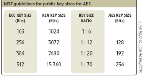
Elliptic Curve Cryptography (ECC) was proposed as an alternative mechanism for
implementing public-key cryptography in 1985 by Victor Miller (IBM) and Neil Koblitz
(University of Washington) [1]. Public-key algorithms are a method for sharing keys
among two or more participants to form a secure channel. Unlike other popular
algorithms such as RSA
i, Elliptic Curve Cryptography is based on discrete logarithms
that are more computationally expensive to invert at equivalent key lengths [1]. As can
be seen by NIST (National Institute of Standards and Technology) guidelines, in Figure
1, reduced overhead (number of transmitted bits of data) is required for Elliptic Curve
Cryptography in comparison to RSA to achieve the same level of security. Initially, even
though Elliptic Curve Cryptography offered greater security per key bit, its complex
elliptic curve algorithm made Elliptic Curve Cryptography computationally intensive and
thus it was not widely used. Since initial implementations, there has been a large amount
of research focused on discovering more efficient algorithms to improve the overall
[image:13.612.202.444.537.666.2]performance of Elliptic Curve Cryptography.
Elliptic Curve Cryptography has been included in commercial standards such as
ANSI (American National Standards Institute), IEEE (Institute of Electrical and
Electronics Engineers), and NIST (National Institute of Standards and Technology) [2].
Beyond the commercial standards, there are currently three National Security Agency
(NSA) Suite B public key algorithms that are based on Elliptic Curve arithmetic methods.
These public key algorithms are; Elliptic-Curve Menezes-Qu-Vanstone
(ECMQV), Elliptic-Curve Diffie-Hellman (ECDH), and Elliptic-Curve Digital Signature
4
Chapter 3
Elliptic Curves
This section first discusses elliptic curve groups and how they are formed,
followed by elliptic curve point representations. Next is a discussion on the state of the
art in elliptic curve research. This is followed by an introduction to the graphical
representation and the algorithm chosen for the elliptic curve addition, elliptic curve
double, and elliptic curve multiply functionality.
3.1. Elliptic Curve Groups
Elliptic Curve Cryptosystems require the use of abstract algebraic groups.
Together with elliptic curve geometry, these arithmetic set definitions are used to form
elliptic curve groups. A group is a set of elements that are closed under a mathematical
operation called the Group Function or Group Operation. For elliptic curve groups, the
Group Operation is defined geometrically. By definition, the Elliptic Curve Group
Operation is chosen to be associative and discrete. The number of member elements is
constrained to a finite number of curve points while still remaining closed under the
Group Function. Lastly, each curve contains an inverse element and an identity element.
Elliptic curve groups can be generated with the underlying fields of F
p(
where p is
a prime
) and F
2m (
a binary representation with 2
melements
) [1]. An elliptic curve must
satisfy the equation
y
2=
x
3+
ax
+
b
, where
a
and
b
are constants satisfying
3.1.1 Groups over Real Numbers
An elliptic curve over real numbers can be described by a set of points (x,y)
satisfying the equation
y
2=
x
3+
ax
+
b
where
x, y, a
, and
b
are real numbers. Each
choice of
a and b
will generate a different elliptic curve. For example, the curve that has
a = –3 and b = 1 is shown in Figure 2. If x
3+ ax + b contains no repeated factors, or
equivalently if
4a
3+ 27b
2is not equal to 0, then the elliptic curve
y
2= x
3+ ax + b
can be
used to form a group, along with the point of infinity, O [1]. Calculations using real
numbers are slow and inaccurate due to rounding errors. Elliptic curve cryptosystems
require fast and accurate arithmetic; therefore, real numbers are not used in elliptic curve
[image:16.612.204.443.360.621.2]cryptosystems.
6
3.1.2 Groups over Binary Fields
The elements of binary fields, F
2m, are represented using a polynomial basis
representation with reduction polynomial f(x) [2], thus the elements are m-bit strings. An
elliptic curve over F
2m is specified by the coefficients a and b which are elements of F
2m
of the defining equation
y
2+ xy = x
3+ ax
2+ b
. The elliptic curve includes all points
(x,y) which satisfy the elliptic curve equation over F
2m (where x and y are elements of
F
2m ). An elliptic curve group over F
2m consists of the points on the corresponding
elliptic curve, together with a point at infinity, O [1].
3.1.3 Groups over Prime Fields
The elements of prime fields, F
p,use the numbers from 0 to p – 1, and all
calculations are completed by performing a modulo reduction by p. An Elliptic Curve E
over prime fields, F
p,is the algebraic curve described by a set of points (x,y) satisfying
the equation
y
2mod p
=
(x
3+
ax
+
b)
mod p
where
a
,
b
are elements of F
p.The number
of points on the elliptic curve over F
pis
nh
, where
n
is prime and
h
is called the cofactor.
NIST recommends these elliptic curves over prime fields: F
192, F
224, F
256, F
384,
and F
521. The 384-bit NIST Elliptic Curve over the prime field F
pwhere
p = 2
384– 2
128– 2
96+ 2
32– 1,
a =
–
3, h = 1, n
and
b
are also provided. The
focus of this thesis will be on the NIST curves over prime fields.
3.2. Elliptic Curve Point Representation
A point on an elliptic curve may be represented by multiple point coordinate
represented as (x
A, y
A). Projective points are represented as (X, Y, Z) which can be
converted back to the Affine coordinate system using the equations x
A= XZ
-1and
y
A= YZ
-1. Jacobian coordinates are represented as (X, Y, Z), Modified Jacobian
coordinates are represented as (X, Y, Z, aZ
4), and Chudnovsky Jacobian coordinates are
represented as (X, Y, Z, Z
2, Z
3). These three coordinate systems can be converted back
to the Affine coordinate system using the equations as x
A =XZ
-2and y
A= YZ
-3.
Affine coordinates are used for communication between any two parties because
they require the lowest bandwidth of all the coordinate systems. Thus, all calculations
performed in other coordinate systems must be converted back to Affine coordinates for
the communication process. However, the Affine coordinate system by itself is highly
inefficient to perform the elliptic curve multiplication and the elliptic curve doubling
because inversions would be required. Inversions are computationally more expensive
than multiplication or addition.
The Affine Coordinates can be efficiently changed to any of these other
coordinate systems by setting each of the Z’s (Z, Z
2and Z
3) to 1, and
a
Z
4to
a
(the elliptic
curve parameter). Converting any of the other coordinate systems back into Affine
Coordinates is computationally expensive due to the necessary inversions (x
A =XZ
-1and
y
A= YZ
-1, and x
A =XZ
-2and y
A= YZ
-3).
All NIST Elliptic Curves are defined by the elliptic curve parameter
a = –3
. The
choice of
a = –3
for the NIST curves was made because it produces a faster algorithm for
8
Since the research defined in this paper focuses on the NIST Elliptic Curves a
combination of Jacobian and Affine coordinate systems will be used for the EC double
and EC addition functions.
3.3. Elliptic Curve Operations
The actual algorithms described in Algorithm 1 through Algorithm 4 are based on
the research described in section 3.3, and thus are those used in this implementation. The
actual C-code written to perform the elliptic curve operations can be found in the
Appendix, A.2, which follows the Finite Arithmetic Assembly Routines.
3.3.1 Point Addition
Graphically, the addition of two points (P + Q = R) on a curve is a simple
concept. To start, simply draw a line between the two points, P and Q. This line will
intersect the curve at exactly 1 more point, –R. Reflect –R across the x-axis and this new
point is R. See Figure 3 for an example. It should be noted that every point, P on the
curve contains a reflection, -P across the x-axis. Thus, elliptic curves are reflective
Figure 3: Point Addition [1]
Adding the points P and –P is a special case. When a line is drawn between P and
–P it is vertical, and therefore never again intersects the elliptic curve. By definition, P +
(-P) = O, the point of infinity. As a result of this, P + O = P, thus making O the additive
10
Figure 4: Adding P and –P [1]
According to [2], [3], and [4] the most efficient software algorithm for adding
points on a NIST defined elliptic curve over F
pis performed using a combination of
Jacobian and Affine Coordinates. However, [4] provides additional steps if both
coordinates are in Jacobian format. If the 2
ndparameter of [4] is modified from an Affine
coordinate to a Jacobian coordinate, making
z = 1
, the algorithms are equivalent because
when
z = 1
, steps are eliminated. Based on [2], [3], and [4], the elliptic curve point
addition function, P(x, y, z) + Q(x, y) = R(x, y, z) for this thesis was written in software
Algorithm 1: Point Addition using Jacobian and Affine Coordinates P(x, y, z) + Q(x, y) = R(x, y, z)
A = Q
x+ P
z2B = Q
y+ P
z3C = A – P
xD = B – P
yR
x= D
2– (C
3+ 2 P
x* C
2)
R
y= D * (P
x* C
2– Rx ) – P
y* C
3R
z= P
z* C
3.3.2 Point Doubling
Similarly to graphical point addition, graphically doubling a point P + P = 2P = R
is also a simple process. At point P, a tangent line is drawn. As long a P
yis not 0, the
tangent line will intersect the elliptic curve at exactly one other point, –R. Reflecting –R
across the x-axis yields the new point of R. Refer to Figure 5 for an example. It should
12
Figure 5: Point Doubling [1]
If P
yis equal to 0, then the resulting tangent line will be vertical, and will
therefore never intersect the elliptic curve. In this case 2P = O, the point of infinity, and
Figure 6: Point Doubling when Py = 0 [1]
According to [2], [3], & [4] the most efficient software algorithm for doubling a
point on a NIST defined elliptic curve over F
pis performed using Jacobian Coordinates.
The resulting elliptic curve double routine, 2P(x, y, z) = R(x, y, z), was written in
software as follows:
Algorithm 2: Point Doubling using Jacobian Coordinates, 2P(x, y, z) = R(x, y, z)
A = 4P
x+ P
y2B = 8P
y4C = 3(P
x– P
z2) * (P
x+ P
z2)
R
x= – 2A + C
214
3.3.3 Elliptic Curve Point Multiplication
Point multiplication is defined as kP, where k is a scalar, or integer, and P is an
elliptic curve point. Point multiplication is the basis of Elliptic Curve Cryptography and
consists of a series of point additions and point doubles. These operations are where a
vast majority of computation time is spent. Algorithm 3 shows the basic method for
point multiplication using a random component, R = kP.
Algorithm 3: Point Multiplication – binary method R = kP
R gets P
For all bits(i) of k
R gets 2R (Point Double)
If k(i) = 1
Then R gets R ++ P (Point Addition)
End For
Return R
Algorithm 3 is one elliptic curve multiply which, for the 384-bit NIST curve,
By adapting the Lem-Lee technique [8] the algorithm can be rewritten to be two
smaller elliptic curve multiplies by:
•
Breaking k into two pieces k
1and k
2such that k
1and k
2when concatenated
together form the bits of k, that is k = k
1| k
2.
•
Precalculating 2
192x P, that is double P 192 times.
•
The computation of R can then be written as:
o
R = k
1** (2
192x P) ++ k
2** P
Where ++ represents an elliptic curve add and ** represents an
elliptic curve multiply
These multiplies can be combined using the method of Shamir as modified by [9].
In the equation above, 2
192x P and P are two points on the elliptic curve and k
1and k
2are
two scalar values. This algorithm works by precomputing the elliptic point, 2
192x P, and
computing k
1** (2
192x P) ++ k
2** P all at the same time using the double and add
process. This process is illustrated as shown in Algorithm 4.
If P is constant, and only k changes, then the values (2
192x P) and ((2
192x P) ++
P) can be pre-calculated and stored in memory in Affine format. Since (2
192x P) is P
doubled 192 times, the savings is much more profound if P is constant since the number
of elliptic curve double necessary is decreased by 50%. If P is not constant, these two
values may be calculated at the beginning of the function and then used in the loop.
However the number of savings is greatly diminished since the number of doubles
remains the same as the basic elliptic curve multiply routine. For most key exchange
16
Algorithm 4: Point Multiplication – Lem-Lee and Shamir’s R = k
1** (2
192x P) ++ k
2* P
Read (2
192x P) and ((2
192x P) ++ P) from memory
If the MSB of k
1= 0 & MSB of k
2= 0
Then repeat this step with next MSB of k
1& MSB of k
2Else if MSB of k
1= 0 & MSB of k
2= 1
Then Set R = P
Else if MSB of k
1= 1 & MSB of k
2= 0
Then Set R = (2
192x P)
Else – MSB of k
1= 1 & MSB of k
2= 1
Then Set R = ((2
192x P) ++ P)
For all bits(i) of k
1& all bits(i) k
2R gets 2R (Point Double)
If k
1(i) = 0 & k
2(i) = 0
Do nothing
Else if k
1(i) = 0 & k
2(i) = 1
Then Set R = R ++ P (Point Addition)
Else if k
1(i) = 1 & k
2(i) = 0
Then Set R = R ++ (2
192x P) (Point Addition)
Else – k
1(i) = 1 & k
2(i) = 1
Then Set R = R ++ ((2
192x P) ++ P) (Point Addition)
End if
End For
Algorithm 4 requires 191 elliptic curve doubles, and on average, 144 elliptic
curve additions for the 384-bit NIST curve. Using this process reduces the number of
doubles by ½, and the number of adds by ¼ as compared to the basic elliptic curve
R = kP algorithm depicted in Algorithm 3. Another important point is that each of the
values added to R (P, (2
192x P), and [(2
192x P) ++ P] ) can not only be precalculated, but
may also be stored in Affine format, working nicely with the point addition which is
faster if one parameter is an Affine coordinate.
The process presented using the Lem-Lee [8] technique required the
pre-calculation of (2
192x P) and ((2
192x P) ++ P). Since this value is the same for all random
component calculations, it can be computed once and stored for later use. To reduce
computation times further, additional values can be pre-computed and stored. To use this
process, the random number k is broken into 4 parts k
1, k
2,k
3, & k
4.This would require
16 pre-computed values to be stored in memory. Each of the pre-computed values would
be stored in memory as an Affine point of the size of the curve being used. Thus, using
the 384 bit curve, 32 384 bit numbers would need to be stored (16 x and 16 y
components). Using this method could reduce computation time by almost 50%, but
18
Chapter 4
The ARM946E Processor
The ARM946E is a 32-bit RISC processor core for embedded applications. It is a
product offered by ARM Limited. This processor is optimized for embedded
applications which require high performance, low cost, small die size, and low power
consumption. The processor uses a 5 stage pipeline: fetch, decode, execute, buffer/data,
and write-back. The 5-stage pipeline achieves 1.1 MIPS/MHz, and approaches a single
instruction per clock cycle.
The ARM946E processor core contains the enhanced DSP capability of the
ARM9E-S processor core. The ARM9E-S processor core executes the extended
ARM5vT instruction set which includes multiplier and saturating arithmetic functions.
Multiply instructions are processed faster using a single-cycle 32x16 implementation.
There are both 32x16 and 16x16 multiply instructions, and the pipeline allows one
multiply to begin each cycle.
The ARM946E supports an external Tightly-Coupled Memory (TCM) for both
instruction and data that can range in size from 0KB to 1MB. The TCM is made up of
SRAM and the minimum size, when it exists, is 4KB incrementing in powers of 2 (ex.
8KB, 16KB) up to 1MB. TCM size is defined once embedment occurs. This memory is
capable of returning data to the ARM9E-S core in a single cycle (no wait states).
Also implemented within the ARM946E are two cache memories, one for
instruction and one for data. Like the TCM, the caches are also made up of SRAM and
can range in size from 0KB to 1MB. The sizes of the data and instruction cache can be
powers of 2 up to 1MB. The caches connect to the ARM9E-S core through 32-bit buses
and allow the pre-fetch of one instruction each cycle. This allows the Load And Store
Multiple instructions to transfer one register per cycle. Cache lock-down is provided to
allow critical code to be locked into cache, which ensures predictability for the code. The
cache replacement algorithm is programmable and may be selected to be either pseudo
random or round-robin. Cache entries are added on a read miss basis. The write policy is
also programmable and may be write-back or write-through.
The ARM9E-S processor core contains 31 general purpose registers, 16 of which
are visible to the user at any one time. The remaining registers are used to speed up
exception processing. Register 15 is used as the program counter, R14 contains the
return address following a subroutine call, and R13 is used as the stack pointer.
Another important feature of the ARM946E is that it contains two instruction sets.
It implements both the traditional 32-bit wide ARM instruction set and the 16-bit Thumb
instruction set. The Thumb instruction set encodes a subset of the 32-bit ARM
instructions, and removes the limitations of code density and performance from narrow
memory. Thumb instructions are basically compressed ARM instructions which are
decompressed at execution time, and then executed as ARM instructions on the
processor. The decompression is simple and performed on the fly without additional
cycles. Thumb instructions have higher performance than ARM instructions on a
processor with a 16-bit data bus, but lower performance on a 32-bit data bus. Thumb
mode is ideal for memory constrained systems; on average the same C code is about 30%
20
The processor is capable of switching between ARM and Thumb mode, although extra
code, called veneer, is sometimes necessary to carry out the transition.
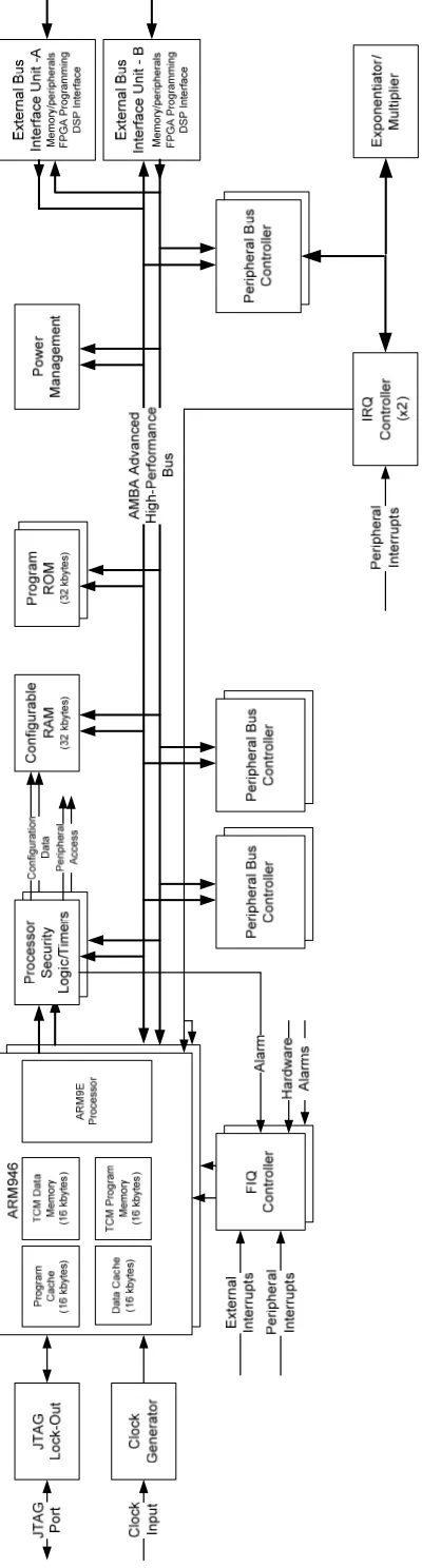
4.1. The ARM946E Embedment
The block diagram for the ARM946E embedment utilized for this thesis is shown
in Figure 7. Internal memory available includes 16 Kbytes of TCM for instruction use
and 16 Kbytes of TCM for data use. The Cache includes 16 Kbytes and is set up as 4 -
way set associative using pseudo random cache replacement and write-back. Cache may
be enabled for CRAM or external SRAM, but not TCM since accesses to the TCM
already contain no wait states.
On the AMBA bus is 32 Kbytes of CRAM (Configurable Random Access
Memory). Interfacing to the EBIU (External Bus Interface Unit), which is also connected
to the AMBA, are flash and more SRAM. Additionally, within the ARM processor are
16 Kbytes of data cache and 16 Kbytes of instruction cache. The ARM946E embedment
utilizes an AiMEC Montgomery Exponentiator Core which is attached to the peripheral
bus controller and interfaces to the AMBA bus. Both the processor and the exponentiator
core run at 100 MHz.
21
[image:32.612.153.353.26.770.2]Figure
7: ARM946E Embe
dment with P
eripherals
Im
ag
e pr
ovided by
Harris Cor
por
22
4.1.1 The AiMEC Montgomery Exponentiator Core
The AiMEC Montgomery Exponentiator Core used in this implementation is
capable of three independent modes of operation:
1.
Montgomery Exponentiation: x = a
emod n
2.
Modular Multiplication: m = ( p * q ) mod n
3.
Modular Addition: s = ( p + q ) mod n
4.1.1.1
Modular Exponentiation
Exponentiation involves solving the equation x = a
emod n. Restrictions apply to
each a, e, and n. The width of a and n, in bits, may be as large as 4096 bits, and the width
of e must be less than or equal to 2048 bits. The value n must be odd.
The exponentiator core utilizes the Montgomery product algorithm, which
contains a very important feature in that it involves a series of mathematical operations
mod r, where r is a power of 2. The inclusion of the mod r function precludes the need
for binary division, which can be costly in both gates and time. However, this technique
requires the pre-calculation of constants derived from the original numbers a, e, and n.
These constants are defined as:
a” = a * r mod n
x” = r mod n
n’ = (r * r
-1- 1)/n
Wherever possible, a”, x”, and n’ were precalculated as soon as a and n were
available. The generation of these precalculated constants is computationally expensive
to do in software, and decreases the overall performance of the system.
The AiMEC Montgomery Exponentiator Core is not an optimized mathematical
core, thus all exponentiations with the same number of bits for the base and modulus will
take the same amount of time. Each Montgomery exponentiation with a base and
modulus of 512 bit, or less, and an exponent of 512 bits, or less, takes 2.1 mS.
4.1.1.2
Modular Multiplication and Addition
The multiplication operation as defined by m = (p * q) mod n, and addition
operation as defined by s = (p + q) mod n, utilize an n whose bit width can be as large as
4096 bits. The length of p and q must be equal to or less than the bit width of n. It is not
required that p and q be less than n in magnitude, nor is there a restriction that n be odd.
For each multiplication using a 384-bit modulus, the time to perform each
multiplication is constant. According to [11], and collected timing, a modular
multiplication with a modulus size of 512 bits, or less, takes
95 uS.
Another inefficiency of this embedment with the AiMEC Montgomery
Exponentiator Core, is that a software modular reduction is necessary if the length of
either operand (p or q), in bits, is greater than the length of the modulus (n), in bits. If p
or q has a most significant bit of 1, and the most significant bit of n is 0, the results of the
24
4.1.1.3
AiMEC Montgomery Exponentiator Core Summery
This AiMEC core is not an efficient mathematical core for performing fast elliptic
curve operations. The necessity to precalculate values for an exponentiation or perform
software modular reduction prior to an addition or multiplication is impractical.
However, on this system, it is still faster than the software implementations for
Chapter 5
Finite Arithmetic Design and Test Setup
5.1. Finite Arithmetic written for the ARM946E
The AiMEC Montgomery Exponentiator Core is unable to perform non-modular
multiplication, non-modular addition, and modular subtraction; C-code was used to
perform these operations. While the C-code worked, it was not as efficient as necessary,
and updates were made to allow for faster execution of the finite arithmetic.
For a modular multiplication, checks were added to determine if either of the
input parameters is equal to one (since many of the z parameters could be equal to one).
If so, a copy is performed in software rather than performing the modular multiplication
using the AiMEC Montgomery Exponentiator. Checks were also added to determine if a
modular reduction is necessary before attempting to perform the reduction in the modular
subtraction routine.
The ARM946E contains the enhanced DSP capability of the ARM9E-S processor
core which executes the extended ARM5vT instruction set, and includes the enhanced
multiplier and saturating arithmetic functions. Writing assembly functions to perform the
addition and subtraction of arrays, as well as 32-bit by 32-bit multiplies was better able to
26
Included in the extended ARM5vT instruction set is the ability to perform a 32-bit
by 32-bit multiply and obtain a 64 bit result with one instruction. By adding this
instruction, plus the storage instructions to an assembly function, an entire C-routine was
removed from the original finite arithmetic C-code. The assembly function, along with
the description and inputs can be seen in Algorithm 5.
Algorithm 5: Assembly Routine
mult_32;****************************************************************************** ;
; Description: Performs the multiplication of two 32 bit unsigned integers ; and stores the product.
;
;ARGUMENTS: r0: Multiplier ( 32 bits ) ; r1: Multiplicand ( 32 bits )
; r2: address of the Product ( 64 bits )
;****************************************************************************** mult_32
STMFD sp!, {r4-r11, lr} ;save regs and return link
UMULL R3, R4, R0, R1
STR R3, [R2] ; store the lower half ADD R2, R2, #4 ; increment to next location STR R4, [R2] ; store the upper half
LDMFD sp!, {r4-r11, pc} ;restore regs and return
The other assembly functions written to handle the addition and subtraction of
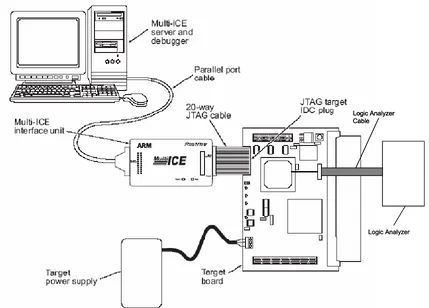
5.2. Test
Setup
A diagram of the test setup is shown in Figure 8. The PC contained the ARM
debugger and ICE software used to walk through and debug the code. The
Multi-ICE interface unit attached the PC to the board. A logic analyzer was attached to a
discrete hardware line that could be toggled during software execution.
Logic Analyzer Cable
Logic Analyzer Logic Analyzer Cable Logic Analyzer Cable
[image:38.612.95.524.266.574.2]Logic Analyzer
Figure 8: Test Setup Diagram
28
Chapter 6
Evaluation and Timing Descriptions
All of the timing measurements performed focused on a 384-bit elliptic curve
multiplication when multiplying an elliptic curve point by a random scalar value. All
measurements were taken using a toggled hardware line and measured with a logic
analyzer as shown in Figure 8.
6.1. Baseline Timing Description
Based on the elliptic curve research, the elliptic curve addition function was
written such that the inputs are one Jacobian and one Affine (refer back to section 3.2 for
definition of Jacobian and Affine formats). The output is Jacobian as shown in
Algorithm 1, i.e., P(x, y, z) + Q(x, y) = R(x, y, z). The elliptic curve double routine uses
Jacobian coordinates for both the input and the output as shown in Algorithm 2, i.e.,
2P(x, y, z) = R(x, y, z). The elliptic curve multiplication routine was written to utilize the
Lem-Lee technique [8] with Shamir’s technique [9] and three precalculated values as
shown in Algorithm 4.
The first timing measurement of the 384-bit elliptic curve multiply routine was
taken and on average took 600 mS to complete. This will be considered the baseline and
can be described as follows:
•
Algorithm 4 was used with a countermeasure to battle side channel attacks
against timing.
•
Instruction and data cache were both used.
•
All of the code was placed in internal TCM.
•
Most of the data was placed in internal TCM, with a limited amount in
CRAM.
•
The code was compiled using the Thumb instruction set.
•
Compiler optimizations were set at the highest level for decreased code size.
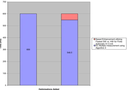
6.2. Hardware Vs. Software Optimizations
With the baseline measurement established, the next step was a comparison to
determine if non-modular multiplication and non-modular addition were faster to perform
in software or utilizing the AiMEC Montgomery Exponentiator Core with a 384-bit
modulus of all 1’s. The software multiplication with the existing finite arithmetic
C-routines was 10 times faster and software addition was 6 times faster than the
exponentiator core with a modulus of all 1’s. It was also determined that if more than 2
modular additions were needed, a single modular multiplication with the AiMEC
Montgomery Exponentiator is faster, i.e. a modular multiply by 8 is faster than
performing three modular additions. Updates were made to the elliptic curve code to use
software whenever a modular reduction was not necessary, and to use modular
multiplication using the AiMEC Montgomery Exponentiator whenever more than 2
modular additions were necessary. These updates decreased the elliptic curve multiply
routine processing time by 51.5 mS and 8.6%, thus the 384-bit elliptic curve multiply
took 548.5 mS on average. Figure 9, shows the original baseline elliptic curve multiply
30
software updates to utilize the fastest approach. The time removed by the optimizations
is included to keep the total execution time at 600 mS.
600
548.5
0 100 200 300 400 500 600 700
Optimizations Added
T
im
e
(
m
S) Speed Enhancement utilizing
Fastest SW vs. HW for Finite Arithmetic 51.5 mS
[image:41.612.102.541.142.454.2]EC Mulitply measurement using Algorithm 4
Figure 9: Elliptic Curve Multiply Baseline and HW/SW Optimization
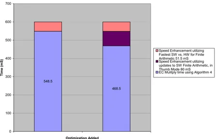
6.3. Finite Arithmetic Software Optimizations
Multiple updates were next made to the finite arithmetic C-routines. First,
assembly functions were written to perform the addition and subtraction of arrays as well
as 32 x 32 bit multiplies. For a modular multiplication, checks were added to determine
if either of the input parameters is equal to 1 (since many of the z parameters could be 1).
using the AiMEC Montgomery Exponentiator. Checks were also included to determine
if a modular reduction is necessary before attempting to perform the reduction in the
modular subtraction routine. These updates removed an additional 80 mS and 14.59%
from the 384-bit elliptic curve multiply execution time, bringing it to 468.5 mS on
average. This is shown in Figure 9. This figure includes the previous updates to make
use of the best software or hardware solution as well as the optimizations to the finite
arithmetic. Each bar in the graph presents the total and component execution times for
the baseline elliptic curve multiply routines prior to the optimizations.
548.5
468.5
0 100 200 300 400 500 600 700
Optimization Added
Ti
me
(mS
)
Speed Enhancement utilizing Fastest SW vs. HW for Finite Arithmetic 51.5 mS Speed Enhancement utilizing updates to SW Finite Arithmetic, in Thumb Mode 80 mS
[image:42.612.102.549.336.624.2]EC Mulitply time using Algorithm 4
32
6.3.1 Finite Arithmetic Library Compiled in ARM Mode
The baseline timing measurement was performed with all the code compiled in
the Thumb instruction set. Compiling the code with the ARM instruction set saved
another 20 mS; however it increased the storage requirement for the code by more than
30% (about 4 Kbytes). The vast majority of the time spent performing an elliptic curve
multiply is devoted to the finite arithmetic routines. Therefore, these routines were
grouped into a separate “finite arithmetic” library and compiled using the ARM
instruction set. The finite arithmetic library was then linked into the elliptic curve code
and compiled using the Thumb instruction set. Given that the library was complied in
ARM mode, and the elliptic curve was compiled in Thumb mode, the ARM/Thumb
inter-working option was also included. The combination of the finite arithmetic library
compiled in ARM, and the elliptic curve code compiled in Thumb, resulted in only an
incremental increase to the code size and decreased the execution time by another 16.5
mS and 3.5%. The resulting execution time for the elliptic curve multiply routine was 452
mS on average. Figure 10, illustrates which enhancements thus far have had the greatest
468.5 452
0 100 200 300 400 500 600 700
Optimizations Added
Ti
me
(
m
S
)
Speed Enhancement utilizing Fastest SW vs. HW for Finite Arithmetic 51.5 mS Speed Enhancement utilizing updates to SW Finite Arithmetic, in Thumb Mode 80 mS
Speed Enhancement utilizing pdates to Finite Library Arithmetic, ARM Mode 16.5 mS
[image:44.612.103.532.99.396.2]EC Mulitply time using Algorithm 4
Figure 11: Elliptic Curve Multiply with Performance Optimizations 2 and 3
To verify that Algorithm 4 was a better alternative to Algorithm 3, the timing was
investigated using the basic elliptic curve multiply routine (Algorithm 3). Here, no
Lem-Lee technique [8], no Shamir’s technique [9], and no pre-calculated values were used.
The previous three updates described and shown in figures 8 – 10 are still included. The
timing to perform the 384-bit elliptic curve multiply subsequently increased from 452 mS
to 646 mS on average, a 30% increase in execution time.
6.4. Compiler Optimization Settings
34
enhancing updates shown in figures 8 -10; the optimizations were changed to increased
execution speed, rather than decrease code size. Each of these enhancements, including
the new optimization for speed, is depicted in Figure 11. The overall execution time to
perform the 384-bit elliptic curve multiply was only decreased by another 6 mS and 1.3%
from an average of 452 mS to an average of 446 mS.
452 446
0 100 200 300 400 500 600 700
Optimizations Added
Tim
e (
m
S
)
Speed Enhancement utilizing Fastest SW vs. HW for Finite Arithmetic 51.5 mS Speed Enhancement utilizing updates to SW Finite Arithmetic, in Thumb Mode 80 mS
Speed Enhancement utilizing updates to Finite Library Arithmetic, ARM Mode 16.5 mS Speed Enhancement made by changing Optimizations for Speed 6 mS
[image:45.612.104.538.226.534.2]EC Mulitply time using Algorithm 4
Figure 12: Elliptic Curve Multiply with Performance Optimizations 3 and 4
6.5. Side Channel Attacks Removed
Next, again using Algorithm 4, the countermeasure described earlier in this
enhancing updates described in the previous paragraphs of this section were included.
The execution time to perform the 384-bit elliptic curve multiply was decreased by
additional 70.5 mS on average to 375.5 mS, another 15.8% decrease.
6.6. Memory
Options
Investigated
To verify that TCM is faster than CRAM, all of the data and code were moved to
CRAM rather than TCM. The time to perform the 384-bit elliptic curve multiply was
increased by 5.6 mS from an average of 446 mS to 451.6 mS on average.
All timing measurements have been performed using the same cache setup.
Instruction and data cache have been enabled for the CRAM. When the data cache was
disabled, the time to complete the elliptic curve multiply routine increased to 472.4 mS
on average. When both data and instruction cache were disabled, the average time
measured was 473.3 mS. After the data cache was re-enabled and instruction cache was
disabled, the time to complete the elliptic curve multiply routine took an average of 446.2
mS. These measurements show that the data cache had very little effect on system
performance, and instruction cache had no impact on system performance. This can be
attributed to the fact that TCM has no wait states and all of the code and nearly all of the
data resided in TCM.
The first bar on the graph which is labeled Alg 4 Optimized, shown in Figure 12,
illustrates the elliptic curve multiply algorithm performance after all optimizations were
applied at an average of 446 mS. It is also shown in Figure 12 that the time to execute
the algorithm was increased when the caching options were changed, or the code is
36
shown in Figure 12 is the amount of time increase to the optimized algorithm
performance when the counter measures are included.
446 446 446 446 446
375.5
0 50 100 150 200 250 300 350 400 450 500
Alg 4 Optimized
I-Cache off D-Cache off Both Cache
off
Code in CRAM not
TCM
Remove Counter Measure
Code Options
Tim
e (m
S
)
Counter Measure Adds 70.5 mS
[image:47.612.100.546.149.472.2]Code in CRAM, Not TCM adds 5.6 mS for a total of 451.6 Both CACHE off adds 27.3 mS for a total of 473.3 mS Data CACHE off adds 26.4 mS for a total of 472.4 mS Instruction CACHE off adds 0.2 mS for a total of 446.2 mS Algorithm 4 With Best Optimizations, 446 mS
Chapter 7
Summary and Future Work
Through the empirical timing measurements, it has been shown that the largest
decrease in execution time was due to enhancements made in the finite arithmetic
functions. These enhancements provided a 22% time reduction in a 384-bit elliptic curve
multiplication. These enhancements included:
•
Rewriting a portion of the finite arithmetic to use assembly functions that
perform the addition and subtraction of arrays and 32 x 32 bit multiplies.
•
Adding checks prior to performing a modular reduction.
•
Using the Exponentiator Core only when modulus reduction was necessary.
•
Using multiplication if more than two additions would be required.
•
Placing the finite arithmetic into its own library and using ARM mode.
Based on the requirements of the system, the side channel attacks could also be
removed. In addition to the 22% decrease in execution time from the previous
enhancements, another 15% reduction in execution time was attained when the
countermeasure for the side channel attack on timing was not implemented.
The other optimizations investigated including: cache usage, compiler options
(speed vs. size), and Thumb instruction set vs. ARM instruction set provided minimal
38
All of the enhancements implemented can be seen collectively in Figure 13. The
baseline elliptic curve multiply routine is shown using algorithm 4 followed by each
enhancement made. The decrease in time from the baseline measurement for each
optimization is depicted using a different color. Once more, it can be seen by the graph
in Figure 13 that the updates made in the finite arithmetic functions provided the most
reduction in execution time.
600
548.5
468.5 452 446
375.5 0 100 200 300 400 500 600 700 Baseline EC Mulitply with Alg 4 Fastest SW vs. HW Updates to SW Finite Arithmetic, Thumb Mode Finite Arithmetic Library - ARM
Mode Optimized for Speed Remove Counter-Measure Optimizations Performed Time (mS)
Speed Enhancement made by utilizing Fastest SW vs. HW for Finite Arithmetic 51.5 mS Speed Enhancement utilizing updates to SW Finite Arithmetic, in Thumb Mode 80 mS
Speed Enhancement utilizing pdates to Finite Library Arithmetic, ARM Mode 16.5 mS
Speed Enhancement made by changing Optimizations for Speed 6 mS
Speed Enhancement made by Removing Counter-Measure 70.5 mS
[image:49.612.67.537.265.598.2]EC Mulitply using Algorithm 4
Table 1 provides a different format to show an overview of all options tested and
the timing achieved. The light blue line indicates the baseline system described in the
third paragraph of the evaluation and timing descriptions. The green lines indicate the
most efficient option found on this system. The difference between the two options is the
use of the countermeasure for a time side channel attack. The percentages indicate the
difference from the base system.
38
4-bi
t E
C
M
ul
tip
ly
T
im
e
av
er
ag
e
(m
S)
A
lg
or
ith
m
4
A
lg
or
ith
m
3
Fa
st
es
t S
W
v
s.
H
W
U
pd
at
es
to
F
in
ite
A
ri
th
m
et
ic
T
hu
m
b
M
od
e
Fi
ni
te
A
ri
th
m
et
ic
li
br
ar
y
A
R
M
C
om
pi
le
r
op
tio
ns
s
et
f
or
T
im
e
C
om
pi
le
r
op
tio
ns
s
et
f
or
co
de
s
iz
e
C
od
e
an
d
da
ta
in
T
C
M
C
od
e
an
d
da
ta
in
C
R
A
M
IC
ac
he
u
se
d
D
C
ac
he
U
se
d
T
im
in
g
C
ou
nt
er
M
ea
su
re
%
s
pe
ed
im
pr
ov
em
en
t
ov
er
b
as
el
in
e
646
X
X
X
X
X
X
X
X
X
-7.6
600
X
X
X
X
X
X
--548.5 X
X
X
X
X
X
X
8.6
468
X
X
X
X
X
X
X
X
22
452
X
X
X
X
X
X
X
X
X
24.67
446
X
X
X
X
X
X
X
X
X
25.66
375.5 X
X
X
X
X
X
X
X
37.42
451.6 X
X
X
X
X
X
X
X
X
24.29
472.4 X
X
X
X
X
X
X
X
21.27
473.3 X
X
X
X
X
X
X
21.12
446.2 X
X
X
X
X
X
X
X
25.66
Table 1: Overview of all options tested
Future work that could be explored includes:
•
A hardware, FPGA or ASIC, version of the elliptic curve and finite
40
•
Usage of an optimized mathematical core that does not return a constant
time for mathematical operations.
Bibliography
[1]
Certicom Corp.
“Elliptic
Curve
Cryptography Tutorial
”, 4 May. 2007. Reference
.com
http://www.certicom.com/index.php?action=ecc_tutorial,home
[2]
M. Brown, D. Hankerson, J.Lopez, and A. Menezes. “
Software Implementation of the
NIST Elliptic Curves Over Prime Fields
”
[3]
M. Hopper. “Mathematical
Routines for Elliptic Curves
”, 21 February. 2001
[4]
Y. Hitchcodk, E. Dawson, A. Clark, P. Montague. “
Implementing an efficient elliptic
curve crypto system over GF(p) on a smart card
”, 24 October. 2002
[5]
H. Cohen, A. Miyaji, T. Ono.
“Efficient elliptic curve exponentiation using mixed
coordinates”
(
http://citeseer.ist.psu.edu/277895.html
), ASIACRYPT 1998
[6]
B. Henhapl.
“
Platform
Independent Elliptic Curve Cryptography over Fp”
[7]
NIST,
“
Recommendation
for Key Management —Part 1:general”
(
http://csrc.nist.gov/publications/nistpubs/800-57/SP800-57-Part1.pdf
), Special
Publication 800-57, August 2005
[8]
C. Lim, P. Lee. “
More Flexible Exponentiation with precomputation
”, Advances in
Cryptology, Proceedings of Crypto ’94, Volume 839, pages 95-107, 1994
[9]
J.Solinas,
“Shamir’s Trick for Elliptic Curves”
, Version 328, 28 March. 2000
[10]
ARM Limited,
“ARM Online Books”
, ARM Developers Suite V1.2
[11]
Flextronics Semiconductor, “
AiMEC Montgomery Exponentiator Core”
,
Specification number 12016-0315
42
[13]
A. Sloss, D. Symes, C. Wright,
“ARM System Developer’s Guide Designing and
Optimizing System Software”
2004
i
RSA is an algorithm for public-key cryptography. It was the first algorithm known to be suitable for
Appendix A
A.1 Finite Arithmetic Assembly Routines
;**************************************************************************** ;
;FUNCTION: mult_32 ;
;LANGUAGE: ARM946E-S Assembly ;
; Description: Performs the multiplication of two 32 bit unsigned integers ; and stores the product.
;
;ARGUMENTS: r0: Multiplier ( 32 bits ) ; r1: Multiplicand ( 32 bits )
; r2: address of the Product ( 64 bits )
;****************************************************************************** AREA Utility, CODE, READONLY
CODE32
EXPORT mult_32
mult_32
STMFD sp!, {r4-r11, lr} ;save regs and return link
UMULL R3, R4, R0, R1
STR R3, [R2] ; store the lower half ADD R2, R2, #4 ; increment to next location STR R4, [R2] ; store the upper half
44
;**************************************************************************** ;
;FUNCTION: add_arrays ;
;LANGUAGE: ARM946E-S Assembly ;
; Description: Performs the addition of two arrays and stores the sum. Also ; increments the length if a carry occurs.
;
;ARGUMENTS: r0: Address of the addend ; r1: Address of the augend ; r2: Address of the sum
; r3: Address of the number of words to add ; also number of words of the result
;****************************************************************************** EXPORT add_arrays
add_arrays
STMFD sp!, {r4-r11, lr} ;save regs and return link
LDR R8, [R3] ; place the number of words to add into R8
MOV R7, #0 ; Zeroize R7 to use to clear and restore the CPSR
add_loop
MSR CPSR_f, R7 ; clear all the flags( 1st time ) OR restore from ADD
LDR R4, [R0], #4 ; place a word from the addend into R4, increment R0 (address)
LDR R5, [R1], #4 ; place a word from the augend into R5, increment R1
ADCS R6, R4, R5 ; add augend, addend and Carry, place in R6, set flags STR R6, [R2], #4 ; store the result into the sum, increment the sum ptr
MRS R7, CPSR ;save the CPSR if to resore before add
SUBS R8, R8, #1 ; Decrement the counter
BNE add_loop ; loop until complete (z flag not set)
MSR CPSR_f, R7 ; restore flags from ADD
BCC add_done ; Branch on no carry (carry clear)
; other wise handle the carry
LDR R8, [R3] ; reload the number of words to add into R8 ADD R8, R8, #1 ; update the number of words of the result STR R8, [R3] ; store the number of words of the result
add_done
;**************************************************************************** ;
;FUNCTION: add_1_to_array ;
;LANGUAGE: ARM946E-S Assembly ;
; Description: Adds 1 to an array and stores the sum. Also ; increments the length if a carry occurs. ;
;ARGUMENTS: r0: Address of the array ; r1: Address of the sum
; r2: Address of the number of words to add ; also number of words of the result
;****************************************************************************** EXPORT add_1_to_array
add_1_to_array
STMFD sp!, {r4-r11, lr} ;save regs and return link
LDR R8, [R2] ; place the number of words to add into R8
MOV R7, #0 ; Zeroize R7 to use to clear and restore the CPSR MOV R5, #1 ; place a 1 into R5 for the 1st add
loop
MSR CPSR_f, R7 ; clear all the flags( 1st time ) OR restore from ADD
LDR R4, [R0], #4 ; place a word from the array into R4, increment R0 (address)
ADCS R6, R4, R5 ; add word from array + 0 or 1 + Carry, place in R6, set flags
STR R6, [R1], #4 ; store the result into the sum, increment the sum ptr
MRS R7, CPSR ;save the CPSR if to resore before add MOV R5, #0 ; place a 0 into R5 for the remaining adds
SUBS R8, R8, #1 ; Decrement the counter
BNE loop ; loop until complete (z flag not set)
MSR CPSR_f, R7 ; restore flags from ADD
BCC done ; Branch on no carry (carry clear)
; other wise handle the carry STR R5, [R1] ; store 1 into the sum
LDR R8, [R2] ; reload the number of words to add into R8 ADD R8, R8, #1 ; update the number of words of the result STR R8, [R2] ; store the number of words of the result
done
46
;**************************************************************************** ;
;FUNCTION: subtract_arrays ;
;LANGUAGE: ARM946E-S Assembly ;
; Description: Performs the subtraction of two arrays and stores the difference, ; also increments the length if a carry occurs.
;
;ARGUMENTS: r0: Address of the minuend ; r1: Address of the subtractend ; r2: Address of the difference
; r3: Address of the number of words to subtract ;
;****************************************************************************** EXPORT subtract_arrays
subtract_arrays
STMFD sp!, {r4-r11, lr} ;save regs and return link
LDR R8, [R3] ; place the number of words to add into R8 MOV R7, #0x20000000 ; bit 29 of the CPSR is the Carry bit, needs ; to be set to 1 to indicate no barrow
sub_loop
MSR CPSR_f, R7 ; update the flags( 1st time ) OR restore from Sub
LDR R4, [R0], #4 ; place a word from the minuend into R4, increment R0 (address)
LDR R5, [R1], #4 ; place a word from the subtractend into R5, increment R1
SBCS R6, R4, R5 ; add sub with carry, place in R6, set flags
STR R6, [R2], #4 ; store the result into the difference, increment the diff ptr
MRS R7, CPSR ;save the CPSR if to resore before subtract
SUBS R8, R8, #1 ; Decrement the counter
BNE sub_loop ; loop until complete (z flag not set)
MSR CPSR_f, R7 ; restore flags from SUB
BCS sub_done ; Branch on no Barrow (carry set)
; other wise handle the carry
LDR R8, [R3] ; reload the number of words to subtract into R8 SUB R8, R8, #1 ; decrement to indicate cary,
STR R8, [R3] ; store the number of words of the result
sub_done
;**************************************************************************** ;
;FUNCTION: sub_1_from_array ;
;LANGUAGE: ARM946E-S Assembly ;
; Description: Adds 1 to an array and stores the sum. Also ; increments the length if a carry occurs. ;
;ARGUMENTS: r0: Address of the array ; r1: Address of the diff
; r2: Address of the
![Figure 2: Elliptic Curve Equation y2 = x3 - 3x + 1 [1]](https://thumb-us.123doks.com/thumbv2/123dok_us/60072.5591/16.612.204.443.360.621/figure-elliptic-curve-equation-y-x-x.webp)
![Figure 3: Point Addition [1]](https://thumb-us.123doks.com/thumbv2/123dok_us/60072.5591/20.612.86.524.79.364/figure-point-addition.webp)
![Figure 4: Adding P and –P [1]](https://thumb-us.123doks.com/thumbv2/123dok_us/60072.5591/21.612.87.524.80.349/figure-adding-p-and-p.webp)
![Figure 5: Point Doubling [1]](https://thumb-us.123doks.com/thumbv2/123dok_us/60072.5591/23.612.91.530.75.349/figure-point-doubling.webp)
![Figure 6: Point Doubling when Py = 0 [1]](https://thumb-us.123doks.com/thumbv2/123dok_us/60072.5591/24.612.89.527.78.341/figure-point-doubling-py.webp)