State-space approach to nonlinear predictive generalized minimum variance control

State-Space Approach to Nonlinear Predictive

Generalized Minimum Variance Control

Mike

J

Grimble and Pawel Majecki

Industrial Control Centr University ofStrathclyde

Graham Hills Building 50 George Street GLASGOW GI tQE

oited Kingdom

Telephone 0: +44 (0)141 -524400 _xtensions: 2378/2880 Direct Line 0: 44 (0) 141 548 2378

Facsimil 0: +44(0)1415484203 Electronic Mail: [email protected]

http://www.icc.strath.ac. uk

Abstract

A Nonlinear Predictive Generuli::ed Minimum Variance (NPG!vfV) control algorithm is introduced

for the control of nonlinear discrete-time multivariable !'J~ystems. The plant model is repre ented by

the combination of a very gen ral nonlinear op rator and also a linear subsystem which can be

open-loop unstable and is represented in state- pac mod I form. The multi-step predictive control

cost index to be minimised involve both weighted error and control signal costing terms. The

solution for the control law is derived in the time-domain using a general op rator representation

of the process. he controller include, an int rnal m del of the nonlinear proce s but because of

the assumed structure of the system the state observ I' is only required to be linear. In the

asymptotic case, where the plant is linear, the controll I' reduces to a state-space v rsion of the

well known GPC controller.

Keywords: State-space, predictive, nonlinear. optimal, minimum variance, transport delay.

Acknowledgements: Ware grateful for the support of the PSRC on the Platform Grant

Proj ct 0 EP/C52642211 and for the usc of the ship model from the Marine Systems Simulator

Introduction

The aim is to design a relatively simple controller for nonlinear s st ms that has some of the

advantages of the popular Generalised Predictive Control (GPC) algorithms. The model based

predictive control (MBPC) approach based on linear theory has been applied very successfully in

the process industries, where it has repeatedly improved the profitability and competitiveness of a

production plant. It has been used to improve performance in difficult systems which contain long

dead times, tim -varying system parameter and multivariable interactions. Predictive algorithms

were initially applied on relatively slow processes (such as thermal processes) for the chemical,

petrochemical, food and cement industri s but are now applied on faster systems, such as servo

systems, h draufic systems and gas turbine applications. pynamic Matrix Control (DMC). due to

Cutler and Ramaker [11 and Generalized Predicti 'e Control (GPC), due to Clarke et. af. ([2], [3])

are popular. Richalet (l4J, [5]) developed some of the first predictive cantrall rs and has applied

the technique successfully in a ide range of applications. The relationship bet een LQ optimal

and predictive control was xplored in Bitmead et al [61. A tate-space version of a GP .

controlkr was obtained in [7].

The solution presented here b lilds upon previous results on Generalised Minimum

Variance (CiMV) control. A Nonlin ar Cieneralized Minimum Variance (NGMV) controller as

derived recently for nonlinear model hased multivariable s, stems b Grimhle ([8J, [9] and

Grimhle and Majecki rIO]. Th tension over the basic NGlv.fV control law involves an extension

of th N;MV cost-index to include future tracking error and control costing terms in a GPC t pe

of problem. When the system is linear the result. revert to those for a GPC controller \vhich i a

valuable solution for many applications. n advantage of the proposed predictive control

hard nonl inearities, a state-dependent . tate-space model, transfer operators or even nonl inear

function look up tables.

The possible advantages relative to other nonlinear predictive control approache can be listed as:

• The general approach is close in spirit to fixed model based control so avoids problems

with on-line linearization and behaviour hould b easier to predict.

• If the system is close to being linear the sy ·tem will b have like a linear GPe control

de ign which is of course similar to DMC and many other well used and accepted

techn iq ues.

• No advanced concepts are needed to d rive the solution presented here and this can be

valuable in gaining acceptance from busy engineers in industry.

The road map for this paper is a follow. The nonlinear plant and linear state-space di turbance

models are described in § 2. It i shown in § 3 that the solution orthe linear multi-step predictive

(GPC) control problem can be lound from the solution of n equivalent minimum variance control

problem. The cost function and the solution of the IJ>CiMV n nlinear optimal control problem are

described in § 4 together with the main theorem. The stability and design issues are consid red in

§ 5 An illustrative design example is presented in § 6. Finally conclusions that may be drawn arc

summari ed in § 7.

System Models

The plant model relating input and output can be grossly nonlinear, dynamic and may have a very

genera! form, how vel', the disturbance signal is a SLImed to have a linear time-invariant m del

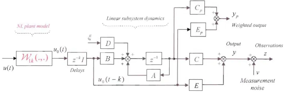
representation. The system il Fig. I includes the nonlinear plant model together with the linear

¢o = Pee +;r;.u + /~'OUO

...

r-y .1

, , _Disturbance

----~:

Pc

:----t~_.---

model

:

_{- - - .}

:

+T+

:

_I

Error I I

I I

weighting ,- - - Control ,- - - -; Input

: f:

I . h . ; F_eG I I h

, we/g t l n g , weig ting

' - _ _ ~ I - 1

I ...

I I

I I

I I

I I

Controller I I

I r

m

Reference I I _-+­

r

+

Nonlinear Linear

subsystem subsystem

Observations signal z v

d

y

+

+

Fig.1: Two Degrees of Freedom Feedback Control System for onlinear Plant

The signals v(t) and ~(t) are vector zero-mean. independent, Gaussian white noise ignals. The

white measurement nOIse signal {v(t)} IS assumed to have a constant covariance

matrix R, = R~ 2: 0 and there is no loss of generality in as uming that the zero-mean white noise

source {~(t)} has an identity covariance matrix. It will be shown that there is no requirement to

pecify the distribution of the noi~e sourc~, since the sp cial tructurc of the sy tcm leads to a

prediction equation, which is only dependent upon the linea!" stochastic disturbance model. The

plant may have a vel' general nonlinear

or

rat I' form.

Nonlinear plant model: ( I)

where z-kJ denotes a diagonal matrix of the common d lay elements in the output signal paths.

The output of the non-linear subsystem Y\.)k will be denoted as

uo(t)=

()!~kU)(t). For simplicity

W_o =:: .k _WOl" is introduced in more detail below and can contain any unstable modes. If ther is

no linear sub-system component then W(j~ = I. The generalisation 0 different delays in different

signal paths complicates the solution but is straightforward 19]. The weighted ou/pu/ equation can

include any stable dynamic cost-function weighting Yp(t) = PC(Z-l)y(t).

Linear Stule-.5'pacl! .)uhsystem Models

The first of the sub-systems to be defined is associated with the linear disturbance model and any

linear sub-system W_o in th plant ode!. Con ider first the linear subsyst ms shown in Fig. 2.

The linear sub-system model in Fig. 2 rna be assumed to b stabilizable and detectable and to be

represent d in the state-space equation form:

.r:(t + 1) == Ar(t) + Bull(t - k) + D~(t) (2)

y(t) == Cx(t) + Euu(t - k) (3)

Yp(t) == Cpx(t) + E ,1L

(t -

k) (4)

1 u

z(t) == G.c(t) + EuuU - k) + v(t) (5)

\ here A. B. C. D, E. CI" E" are (;onstant matric s. The delay free plant transfer of the linear sub­

system, referred to above. may be ritten as lVo~ == E + C<I)/3, wher. <1) = (21 - A) I. The input

signal channels in the plant model are assLim d to include a k-steps delay and the signals may b

listed a-:I:(1) == linear sub-system states; l/u(t) == input ignal to the lin\,;ar subsystem; n(t) =

control signal; y(t)

=

output signal; z(t) == observati n ; r(t) == set-point or reference; Yp(t)

rVeighted OUlPUI

Output Observations

+ Z

v y

+

Linear SlIhsl'stem ,z\'/wmics

.\!. plulI/ //1m}!!!

u(t) _Delays

_ _

---..~EC

+

+,

uo(t-k) ~

'--­

Fig. 2: Nonlinear Plant Input Subsystem and Linear Output and Disturbance Subsystem

Future Outputs and States: uture values of the states and outputs may be obtained as:

xU + i) = A'xU) +

±

A'-/ (Buo(t + j -I-k) + Dc;(I +j -I))

(6)

,~I

The expression for the future states may be obtained by changing the time ir (6) by th k-. teps of

the explicit transport delay giving:

x(t +i+ k) = ....I'x(l + k) +

±

A' I (Bu()(l +

.i -

I) + Dc;U + j + k - I)) (7) I-I

Future Weighted Outputs: The weighted output equation can include any stable dynamic cost­

weighting:tlp(t)

=

p,Jz-J)y(t) , which involves augmenting the st, te quation model. oting (3) th

weighted output y('(t) has the following f rm (for 7. 21):

y/t + i + k) = CpA'x(t

+

k) +

I

C'pA'-J

(Buo(t +

.1-1) + Dc;(t + j + k

-1))

+E,,!Lo(t

+

i) (8)

J-l

Th output arc to b computed lor controL in the interval T E

[t, t

+

N].

Introducing an obvious

notation for these output signals they may be collected in an Nfl vector form as:

[image:7.612.80.555.101.259.2]

Yp(t + k)

Yp(t + l + k)

Yp(t+2+k)

Yp(t + + k)

=

Epuo(t)

E),'Uo(t + 1)

Epuo(t + 2)

Ep'Uo(t + . ) +

CI_p

CAp

C A_p 2

C p18

+

.r(t + k) +

0 CD _p CAD_p

0 0 0

CpS 0 0

CpAB CpB

0 A'\ -lB

p C _p A' -2B _CpB

0 0 ~(t + k)

ueJt)

uo(t + 1)

uo(t+·T-1)

0 0 ';(t+l+k)

D

p (9)

0

AN-1D C A' -2D _CD (t + N -1 + k)

p p p

With an obvious definition orterms this equation may be written as:

where the following vectors and block matrices ma b defined for the case: N > 0:

e r e ('

. =(

_{lag p' I" •• , .}C _{P (} 1 and E'

=

di n!J { E . E , ... , E } (N I square)

P' P ]J

AN

=

1

;12

AN

BN

=

() B AN-In () () 13

A v 2[

0 13 () 0 () ()

D

IV

=

\if!_t.N

=

1:( t)

~(t+ 1)

[f0

1.1

=

'/to(t)

uo(t + I)

Rt,N

(,(/+N-I)

'l/.oU

+ N)

(J 0) 0 U AD AN-1n 0 0 D AN2 D 0 0 0 D

=

'r;,(t) r~(t+1)

(I J)

.,. (t + J

For the special case: N

=

O,A_N

=

I ,B_N

=

D_N

=

o.

eN

=

C_{p '} EN

=

E_{p '} The transfer ~ '\

denote a vector of future white noise inputs and U,.\, denote' a block vector of future control

signals. The block vector R",v denotes a vector of future reference ignals that must include the

same weighting as on the output (8) r~(t) -= Pc(z'l)r(t). The k steps-ahead tracking error, that

includes any dynamic error weighting, may be writt n as:

The 'eighted inferred output to be minimised is assumed to have the same dimension as the

control signal. The matrix

v'v

in (12) for N> 0. is ofa block 10 er triangular form:

E p 0 0 0

CpB

E

p 0

VN

=

GNBN +E,

=

G AN 2B

p

G AN

In

l'

GpB

C AN -2

n

II

Ep

(,'fJ

- !'

0 Ell

(13)

For the special case of a single-slane cost ~

=

0 and thi . matrix must be defined as V_N -= E _p.

Prediction Model

The i-steps ahead prediction of the utput signal ma be calculated by noting the ab ve re ult (8)

then, YpU + i + kit)

=

CpA'i:(t + kit) +

L

1

CpA '-J

Buo(t + .J -1) + EpuoU + i) ( 14)

r 1

where .i:(t + kit) denotes a least squares state estimate from a Kalmanjilter. Collecting results

for the case N> 0 the vector of predicted outputs ~.kN may be obtained in the block matrix form:

Yp(t+k:lt)

Yp(t + 1+ kit)

Yp(t + 2 + kit)

yp(t + N + kit)

=

CI _p CA_p A2 )' CAN ]I '--v----'

i(t + kit) +

E_p 0 0 0

CB

Ji Ep 0

CB

]I C _p A '-2B

C

AN-IB

C

AN _-2B

Ep

cn

0

E

l' P P P

1-t_o(t)

uo(t +1)

uo(t + N)

v ' ' - - - v - - - '

GNA_{N VN ",GNBN}+E'N U~N

(15)

This N+ J step-ahead prediction in (15) can clearly be written in the form:

Y .

N

=

C A".i(

t

+ kit) + VvUo ( 16)

t+k, i"¥ I "J

Output prediction error: - Y;.k N -_, Yt , . , N

- hence. the injerred output estimation error:

where the k steps-ahead state estimation error: ,i:(t + kit) = :r(t + k) - i(t + l.:

I

t) . The state

estimation error IS indep ndent of the ch ice of control action. Also recall that the

optimal.i:(t + f..,;

I

t) and :r(t + kit) are orthogonal and the expectation of th product of the future

mean white noi, e driving signals, is null. It follows that the vector of predicted signals Y:Tk,N In

(16) and the prediction error Y; _., N are orthogonal.

Kalman Estimafor - Predictor Corrector Form

The estimates are r quired from a Kalman filter summari ed briefly as:

x(t

+

I It) = Ax(r

It)

+

BuoU - k) (Predictor) ( 19)

x(r

+

11 t + I)

=

x(r + II t) + Kf ( z(t

+

I) - z(t

+

II

t))

(Corrector) (20)

z(t

+

II

t)

=

Cx(t

+

II

t)

+

£uo(t

+

1-k) (21 )

The state estimate x(t + kit) may be obtained, k steps ahead. using a Kalman filter [II]. In this

form of the estimator the numb r of states in the filter is not increased by the number of the

synchronous delays k, The desired prediction equation:

(22)

where To(k,.:-I)den tes a finite impulse response hlock. To(O,Z-') = land for k ~ I:

ing (19) to (21) the optimal estimate may b written:

xU

+

I

It

+ I)

=

Ax(r

I

t)+ BuoU -k)

+

K, (z(t + 1)-CAx(t 1t)-CBuo(t -k)- t'u()(t + l-k»)

Th~ab ve equation may therefore be written:

where (25)

(26)

Observe that for the Kalman filter to be unbias d the following equation mu t be satisfied:

(27)

This result may be verified u ing (25) and (26).

Generalised Predictive Control Review

A review of the derivation of the CPC controller is provided below where the input _{(1,0) will be}

taken to be that for the linear sub-system. The CPC criterion [12] to be minimised:

J

=

E{

£

e/I

+ j + k)/ e,,(t + j + k) +J..7uo(t + j)' uo(t +

j»1

t} (2S)

/=0

where: E{.jt} denotes the conditional e, pectation, conditioned on measurements up to time t

and A) denote. a scalar control signal weighting actor. The vector of future weighted reference

signal is denoted by

r;,(L

+ j + k) where the weighted error (~p(t;)

=

T~(t) - Yp(t). The future

optimal control ignal is to be calculated for the interval t s

[l,

f +

N].

The state-space models

generating the sionals r, and y" may include any dynamic cost-function w ighting~.(=-').

rllJ.

l

Optimal Cuntrol Solution Using Slale Estimate Feedback

(29)

(30)

where the co,t weightings on the future inputs 11₀ are written a i\~ =diag{A~,AI2,.... A~!}. The

terms in the cost-index can then be simplified, fir t by noting the optimal estimate Y;'k,N 15

orthogonal to the estimation err r Y;-k,N and second by recalling the future refer nee R'+kN IS

assumed to b a known signal over the N+ 1 steps. Simplifying, obtain the vector/matrix form:

Vector form GPC criterion: (31 )

where J_o =:: E{Y,~A ",Y,+k,,\' It}. Substituting from equation (16) f, r the vector of state-estimates:

and riting: (32)

Using these results the cost unctiol may be expanded as:

(33)

The proc~durefor minimising this cost term. if the signals are detcrmini'tic, is almost identical to

that when th conditional cost is con id red. The gradient or the cost-function must be set to zero,

to obtain the vector of future optimal control signals. From a perturbation and gradient calculation

[J2j, noting the J_l1 term is ind pendent of the control, the vector of/illure oplim"f confrol signals:

Th GPC optimal control is defined from this vector based on the receding horizon principle [13]

and the optima) control is taken as the first element in the vector of future cOl1trols [ltUN.

Equivalent Cosl Optimisation Problem

It is now shown that the above problem is equivalent to a sp cial cost minimisation control

problem which is needed to motivate the NPGMV problem introduced later. Let the constant

positive d finite, real symmetric matrix: X_N :::: V;V

N

+

1\~ that enters the above olution, be

factorised into the form: (35)

Observe that by completing the 'quares in equation (33) the cost-function may be written as:

That i , the co t-function: (36)

wh re the signal: (37)

The terms that are independent of the control action ma be written as: ./IU(t)::::./O +./I(t) where,

(38)

Since the last term J1U(t) in equation (36) does not depend upon control action the optimal control

is found by setting the first term to zero, giving the same control as defined in (34). It follows that the 0PC optimal controller for the above linear system is the same as the controller to minimise

Modified Cost-Index Giving GPC Controller

The above motivates the defir ition of a new multi-step minimum variance cost problem that has

the same solution for the optimal controller that i needed before the nonlinear problem can be

considered. A new signal to be minimised involving a weighted sum of error and inputs:

(39)

The vector offuture values of this signal, for a multi-step cost index, may therefore be written as:

()

(40) I ,.

Introduce co t-function weightings, ba ed on the GMVweightings above, to have the form:

~.\, =::

V/;

and (4\ )

which will be justified by the property established in Theorem 3.1 b low. Then motivated by the

preceding, define a new minimum variance multi-step cost-function, using a vector of signals:

(42)

Predicting forward k-sleps (43)

Consider the ignal ¢t+k,N and substitut for the output Y:lk,N ==}~,J,;,N

+

~'k,N' Then from (43):

(44)

This expression may be written in terms of the estimate and the estimation error vector as:

(45)

and the prediction error: _{<f:>t+k ,N}

_{= -}

~'N

_Y;+k,N (46)

Multi-Step Cost Index: The performance index (42) may therefore be simplifi d and written as:

The terms in (42) can b simplified, recalling the optimal estimate ~+k.N and the estimation error

~t-/;;, are orthogonal, and the future reference trajectory

R,...

J.N is a known signal. Thus,

(47)

Thence, the cost-function may be written: (48)

The last cost term in (48) is independent of control action and may be written as:

(49)

This vector <Pt+k,N may be simplified by ubstituting for ~+/;;,N' from (16) and (35):

<P

_~k.N =P (R _{eN IIk,N}

- f )

_{tik,N +} po[o eN' t,1 =1> eN (R l.k,N -(' N r I·A·(t ty.Y . + . klt))-(\!I"V N N + I\.N A2)UOt,N

Thence, from (35) obtain: (50)

Recall the optimal multi-step minimum variance predicf;ve control sets the first squared ferm in

Theorem 3.1: Equivalent Minimum Variance Cost Optimisation Problem

Consider the minimisation of the GPC cost index (28) for the system and assumptions introduced

in §2, wh re the nonlinear subsystem: V\.{k

=

J and the v ctor of optimal

Gre

controls is given by

(34), If the cost index is redefined to have a multi-step minimum variance form (42)

weightings

Pc", =

V;

and J';~.

= -

\~,

,

then the vector of future optimal controls is identical to the

GPC controls in (34).

•

Solution: The proof follows b collecting the results in the ection above.

•

Nonlinear Predictive GMV Control

The actual input to the system is the control signal u(t), hown in Fig. I, rather than the input to

the linear sub-system _uo' The cost-function for the nonlinear contI' I problem of interest must

therefore include an additional control signal co ting term, although the costing on the

intermediate signal uo(t) can be retained to e, amine limiting \.:ascs. If the small t delay in each

output channel of the plant is of magnitude k -steps this irnplie' the control affects the output

k-steps later and the control costing should include the dclay(~u)(t)=:: k (f;:kU)(t). This weighting

on the nonlinear sub-sy'tem input will be assumed to be full rank and invertible and can be a

linear dynamic operator but it may also be chosen to be nonlinear [11J. Thw, consider a new

signal to be minimised: ¢()(!) = p".e(l) + Fcouo(t) (;Z;:U)(l) (51 )

A multi-step cost index may now be defined that is an extension of the cost-function in (42).

The signal <D~+k,N is defined to includ the future control signal costing terms:

where the non-linear function ~k,N t,N will normally be defined to have a simple diagonal form:

(54)

and the vector of inputs: Ut~N = (Y1{k,NUt")' where Y1{k,l\ also has a block diagonal matrix form:

(55)

The problem simplifies when N = 0 to the single-step NGMV control problem.

The NPGMV 'antral Prohlem Solution

The solution follows from very similar steps to those in §3.3 and will therefore be summarised

briefly, Observe from (43) that <Do =cD + z-k.T."NUt and (D~+kN=<D~+kN 1,<D,o'.Lvwhere

t,N t.,v C,,-,..N • , .

<i>U =

cD

+.T.U = P (R -

Y )

+ F U

UO +.T U (56)

, ... k.N tlk.N "k,N L.N C'N t.k,N L+k,N (:N toN "k.N t.<

The estimation error: (57)

The future predicted values in the signal: <i>~+k,N involve' th e timatt:d vector of weighted outputs

~tk,N and these are orthogonal to }~'k.,\' ote the estimation error is zero mean and the expected

value of the product with any known signal is null. The cost-function may therefore be written as:

(58)

(59)

/vPGA1V Optimal Control

The v ctor of future controls follows from the condition for optimality in (59):

u =-

(7 - A2W )-1 P (R -

Y

)

(60)

t,,," ck,N N lk.:>' cO' l+k,N IJk,N

A solution of (59), that is useful for implementation becomes:

(61 )

The optimal predictive control law is nonlinear. since it involves the nonlinear control signal

costing t rm .T::..k,N and the nonlinear model for the plant J1{k,N' Further simplification [s

possible by substituting from (16) for~+k,N'since quation (59) may be written as:

or (62)

This condition fhr optimality i the equivalent f that stemming from (50) hut with the;z:;; ',N is

added. T 0 alternative solutions for the vector a/future optimal controls, in terms of the estimate

of the future predicted tate. therefore becom :

(63)

or U _t.N

=

-.T_k-I _I/~•r (P.,(R _{(/\ t t - " ' d '} "V - lNA,y:/;(t + kit)) - XNW_lk

JJ )

(64)

, I ' t,N

Remarks: The control law is implemented using a receding horizon philosophy and it b comes

zero (~k,N ----:; 0 J1{k,N

=

I). From (63) if the control weighting ~k,N----:;0 then !.N will

introduce the inverse of the plant model Y1{k,~ (if one exists) and the r suiting vector of future

controls Ut~N ill then be the same as the GPC comrols for the linear system that remains.

Optimal Nonlinl:'ar Predictive Control Signal

These expressions can be simpli led further by substituting for the expression for the optimal

predicted state in (22) and invoking the condition for optimality in (62):

Recall uo(t)

=

J1{kU(t) and vrite: ( 5)

The alternative form for the condition for optimality follows as:

(67)

An alt rnativ xpres ion also follows from (66):

To impl ify the equations also introduce the constant matri x:

(69)

Condition for optimali~ll: Equation (66) may be written as:

Optimal control: Two possible expressions for the vector of future optimal controls folio

(71 )

Theorem 4.1: J. PGMV Optimal Controller

Consider the linear components of the plant, disturbance and output weighting models in state

space form (2), (3) with input from the nonlinear finite gain stable plant dynamics

Y\.ik'

The

multi-step predictive control co t-function to be minimised, involving a sum of future cost terms.

is defined in vector form as: J

=

E{<p°T

et>0

I

t}

(73)

P f+k,N f+k,

where N> 0 and the signal <f>~+k,N dep nds up n future error, input and nonlinear control signal

costing terms: <f>0 _tck,N

=

P E _{CN t+k,N} +

FO

_{oW t,N}

°

+.T _ck,N U _t,N (74)

The error and input cost-function weightings are introduced as in the GPC problem (28) and these

determine the block matrix cost forms

P,,,,

=

v'0

and F;0, :=: -A~,. The control cost weighting may be

nonlinear and has the fonn

(f;:U)(/)

:=:

(y:;:-kll)(

t - k) , where k represents the transport dela and f;:k

is full rank and invertible. Define the constant matrix X_N

=

V~'vN

+

A~ then the j f'GMV ptimal

The current control can b computed lIsing the receding horizon principle from the first element in

the alternative expression for the vector o/future optimal controls:

•

Solution: The proof of the optimal control was given bef< re the Theorem and the assumption to

ensure closed loop stability is explained in the stability analysis below.

•

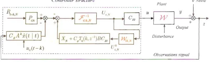
Remarks: The expression (76) leads to the structure in Fig. 3 which is useful for implementation.

This involves a Kalman predictor stage and note that the order of the Kalman tilter depends only

on the d lay free linear subsystems and not the channel delays. If the output weighting Pc includes

a near integrator it appears in the feedback and reference channels and it is desirable to move this

integrator term into the common path. The cost-index (74) when the input costing FU

j nul! eN

and in thi case<p;ltk,N

=

F~'EI+k,,y + (~k,i!IJ. Th limiting case of the NPGtvIV c ntroller is

therefore related to an NGAifV control I r wher the error weighting is scaled by the E1 ' term.

p

('ontroller sfrut'tllre v /Voise

Plant

,---~

~~N + ; _'f­

p'-p

+ :

,

,

'---.:

I ,

,

,

II (/-k) UO_N :

l o t , I

1 • ~

i­

Output

Observmions ,~iRnal

[image:22.612.103.506.596.715.2]

Noise

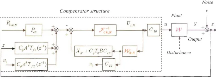
]I Compensator structure

y Z

+ + Output Plant Disturbance + + ---, ,

: R!+k,N

,

:---toI

: l - - _ - - '

, ,

, , L.

-, , , , , ,, , , ,

Fig. 4: NPGMV Compensator in Estimation Future Controls Form

Stability of the Closed Loop and Design Issues

To c nsider stability properties a different expr ssion is required for the cantI'l action where the

results are expressed in closed loop operator forlll. An algebraic result is fir t required involving

erms from the Kalman filter equations. Recall from (27):

but from (23) To(k,z 1)=(l-Akz-k)(=T-Afl. Usingth seresultsandnoling WOk =E+CC!>B,the

de ired result is obtained a :

C... T (I. I)fl (' 4 kl' ( 1) r< ,'kT" ( I) kHr ' ' ' ' ( l)fl ₍₇₇₎

/,! U r.: l Z ,¢' /2 Z +l q,''i /l Z Z n Ilk = '~4! Z

Assumptions and Closed l.oop Expressions

For lin ar GMV de iglls stability is ensured when the ombination of a control weighting and an

error w ighled plant model transfer is strictly minimum phase. For the proposed nonlinear

[image:23.612.96.526.102.260.2]

upon the assumption of stability on the nonlinear plant sub-system U(k. For this stability

discussion assume that the stochastic inputs are null. Then

z(t)

=

Cx(t)

+

Euo(t -

k) +

'o(t)

---+ (E +

Cet>B)uo(t - k),

and the optimal control b comes:

Substituting from (77):

(78)

The control costing is normally a linear model and under this a 'sumption (78) corresponds to the

following condition for op imality:

(79)

where (YV;k.} t

J

= [(YV;k'u)(tf, ... ,(YV;kU)(t + N)T

f·

The desired expressions for the vectors of

future optimal control' ,md nonlinear plant sub ystem Ot tputs therefor become:

Future controls:

NL Subsystem future outputs:

(8t)

Total NL future plant outputs:

Stability Condition and Cost Function Weightings

linear plant sun-system is open loop stable all the operators in (80) to (82) are stable. If the open

loop plant is not stable then further assumptions are need cd to guarantee the stability of term In

(82).

[f there exi ts a PID controll r that will stabilize the nonlinear system. without transport

delay elements, then a set of cost weightings can be defined to guarantee the exi ·tence of this

inverse and hence ensure the stabiJ ity of th closed-loop. As ume that only the error and control

weighting are used. nd that the input weighting A~ --) (). Thcn

X

N

=

V~VN + A~v --) V,~V

Recall that in the ingle-step cost problem, wh re N = O. the matrix V

=

"'1 is assumed square

follows that in this limiting case: (83)

Cost Weighting Choice

One of the main problems in nonlinear control is t ensure a stabilising control law and as the

assumption at the start of the main Theorem 4.1 confirms thi depends on the selection of the cost

weightings. A practical method of deriving such weighting. is suggested by these limiting results.

The telm (1 -.;z:;;~lE~·~.V~)kJ1{k) may be interpreted as the return-differenc operator for a

nonlinear syst m with delay-free plant model J1.{

=

WOk J1{k' Thus, if the plant already has a PJD

controller that stabilises this model, the ratio ofweightings (-~kIE;Pe)can be chosen equal to the

PID controller. Then the weightings are linear and satisfy FC-k'E;~.

=

KI'J{)'

Even for a linear GPC design stability is not guaranteed for all cost function weightings. There

will be some ystem descriptions where even scalar non-dynamic weightings mayor not ensure a

table closed-loop d sign. Now if the cost horizon is reduced to one step the cantrall r becomes

equal to an NGA1V design, which can be guaranteed to have a stabilizing solution by a imilar but

simpler method a in the previous paragraph. The argument is then that a' the multi-step cost is

introduced and the horizon increase it is normally the case that predictive c I1trols improve

resp nses. Thus the strategy or starting with a weI[ tuned NGMV solution and then increasing the cost horizon to introduce prcdicti e action is a practical method offinding co t terms that stabilize

Robustness of the Closed Loop System

In the predictive control of linear systems it is usually the case that step response overshoots

reduce as the cost horizon increases. This behaviour is related to smaller overshoots in frequency

domain terms in the sensitivity functions and this sugge ts there is a commensurate improvement

in robustness. Similar re ults are observed in the nonlinear case but robustness and sensitivity

then relates to the sensitivity operators. Th subject of robu tness in the presence of plant

uncertainties does of course deser e much more attention. A possible approach to the analy is of

NPGMV systems is indicated briefly belo....

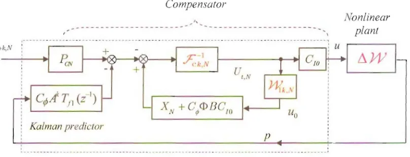
Consider the case of a stable open loop sy tem and note that the relationship (77) can be employed

to show that the system in Fig. 4 can be redrawn as in 'ig. 5 below. This figure is of interest

because it resembles a Smith predictor type of structure but for the present discussion it allows

robustness to be assessed in a patiicular case. eglect for the moment most external inputs and

assume that the plant has an additive uncertainty of he form: W = W + W. Then noting the

signs of the signals summed in the bottom path observe that the diagram in Fig. 5 may be redrawn

as shown in Fig. 6. From this diagram it is clear that the internal feedback loop which includes the

delay free plant model has a signiticant effect on robustness. his loop depend n both the error

and the control signal weighting choices. If for example the system has large high frequ ncy

uncertainty, such as resonances in a mechanical system, then th control costing can include a lead

term introduced at frequencies below the pos ibJe r onant behaviour. The result will be a low

gain in the forward path at high frequencies as determined by the inverse of the c ntrol co ting

within the inn r loop. To ome extent thi weighting acts as a natural so called robustification

filter. Zames (1966, (281) small gain theorem can then be applied to demonstrate that an

-

-Compensator .'vuise

Nonlinear v

'­

---­

---.

z

+

y

+ Output plant

Disturbance

U_t,N

+

+

~

kN

Kalman predictor

p

₊

Observations z

: _ _ • • • • ---_ . ­_ _ -_ • • e • ~ _ • • • • a _ . • • • • !

Fig. 5: onlinear Smith Predictor Implied by NPGMVCompensator Structure

Compensator

Nonlinear

'­

---~ ~---~ plant R_i+k,N

,--­...­--...­--. _.._-­... ---­..­---_. _. ­-_.. ---_.. _. ­....­-_ ...­---....­_. ­_.... _.-­_.._. -"1

u

+

,

+

Kalmun predictor

p

fig. 6: Loop Structure When Additive Uncertainty Present

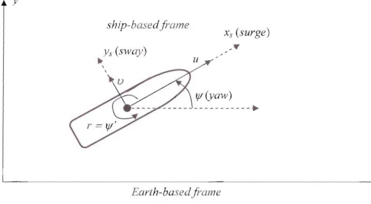
Predictive Control Design for Dynamic Ship Positioning

One of the potential applicati n areas for NPGlvIV control is in dynamic ship positioning and manoeuvring. A desired ship trajectory is often known in advanc (in the case of c~ynamicship positioning. the wntrol objective normally consists in ke .ping the v ssel's position constant,

[image:28.612.86.551.99.296.2] [image:28.612.107.511.396.551.2]

Earth-based coordinate frame, as shown in Fig. 7. The bjective here is to control the vector of

ships position and heading '7

=

(x,Y,Ij/]'

via a thrusters/prop Iler propulsion s stem, so that a

desired trajectory '7r<:1 is followed. This is a well known problem that ha been analyzed in detail

in literature - ee for examplc [14 to 17]. In the following, the NJ'GMV controller is lIsed and

assessed for this application.

Y

ship-basedframe

xs(surge)

,'t/f

Ys (sway)

u

IjI (yaw)

...

---.

Earth-basedframe x

Fig. 7: Dynamic Ship Positioning Problem

System model: The simplified lin ariLcd dynamics of the system are described by the following

di ffer ntial equ tion: Ali, + Dv = r (84)

where M is the inertia matrix, D represents sy. tem damping. v = [u u r( is a ship-based velocity

vector, and T is a vector of force' in X" and 'v',' directions, and the yaw torque. Thi pproximati n IS

valid especially at low spceds and positioning problems. The full nonlinear model, taking into

account Corio1is and nonlinear damping term. is given in [14J.

The velocity vector is related to the Earth-based po itions by the following kinematic

[image:29.612.113.475.265.465.2]

where R(If) is the 3DOF rotation matrix: (86)

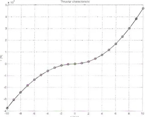
A simple diagonal thruster configuration was a umed in this paper. and the following nonlinear

static model for thru t forces and torq LIe was u d [15]:

(87)

where p is the water density. d is the thru ter diameter, n is the velocity in [rev/s]. and Kr is the

additional nonlinear thruster coefficient. The nonlinear thruster characteristic as a function of n is

shown in Fig. 8. In the following imulation studies. w have u ed models from the Marine

Syst ms Simulator Toolbox for Matlab [18].

x 10~ nvo-ster chara.ctonsllC

r - - ~

-51 _:

r-·

4[ ­

3 -- :--­

-._­

J

J

....

~

_. ,.

t-of

i

.,

~

I

::r

, ,

.... ---'--

-

J

·'0 ·8 -6 .... -2 0 8 10

Il ~1/4i

"

fig. 8: Nonlinear Thrusters Cbaracteristic

Based on the ahove ystcm description, the opl.::n-Ioop Hammer tein model may be eparatcd into

nonlin ar and linear components as shown in Fig. 9. with the black-box model

J1{k

representing

the thrusters. Note that the nonlinear transfi rmation matrix R( Iff) i' not considered part of the

[image:30.612.180.428.368.568.2]

For th controller design, a discrete model of the linear dynamics w s obtained using the Tustin method, with the ample time Ts

=

0.1 sec. A nominal one sample delay (k

=

I) was assumed for

this model.

17£

----+ R(lj/)

11 ₁

_l

'7

-T

•

~) _s J

Thrusters Ship dynamics

Fig. 9: Decomposition of the Ship Model

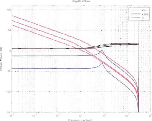
Wave model: The wave disturbance was described using a second order resonant system,

according to the transfer function: w(s)=, k , . where the parameters were defined as: s-+ 2t;OJ"s + (U,;

OJ" = 0.8 rad and t; == O. I. The scaling factor k was chosen '0 that realistic wave amplitudes ere

S

[image:31.612.133.482.188.299.2]

100 .,

,',r:

:r:.

1

~ _.,

100

--I

. - R :

~5oJ ~-~~---~---._----'

~-10· ":1 . H 10 to

f:'roquanq il(tfliliOCj

Fig. 10: Frequency Responses of System Models (plant, disturbance and nominal error weight)

NPGMV Controller implementation: Th structure of the model allows the solution of the

algebraic loop problem to be simplified. Recall the expression for the optimal control equence

(76):

The nonlinear thrusters model represented by J11~ is static and diagonal. while th control

weighting can bC'cparated into a component affected by the current control (the direct through

term) and a part dependent only on the past control values: .J;:k(r)=.r;;(r)+.F:(r), where .J;"(r)

contains a one- tep time-delay (note that a imilar decomposition would apply to a dynamic J1{k

model). Employing block matrix notation to indicate the block-diagonal structure of ';::1-'" the

expression for the vector of future controls can be n:writtcn as:

[image:32.612.181.436.104.306.2]

(88)

Since To(k.z~') contains a one-step time d lay, th right-hand side of (88) involve the vector of

controls computed in th pr vious step, and hence the current control is dependent on the past

controls and inputs and the algebraic loop is removed.

For a practical realization of the control law, it is necessary to invert the static operator

(JL;;,N - XNfiik,N ). Since /~v is in general a fu II matrix. a closed analytical form of the inverse wi II

not normally exi t, even though the M{A,\' nonlinearity i itself invertible. The solution is to sol e

the resulting nonlinear equation on-line. using an it rative Newton method [19]. An alternative is

to insert a memory block inside the ~ edback loop - this leads to a realizable but suboptimal

solution.

The final structure of the controller is as shown in Fig. j I. ote that the actuator saturation limits

have also been includ d in the model.

(',ANA'" -~ P,'N +

-,..

R,.k .N

'7(1)

X/II

Kalmall ~ L...­

-.

iller

* ­

Z

...

­ ~

.r17l

~ U/. N

I--(~.N

- XNU{k,N

)-1

_"b1.J

+

-.;:;.

\

+-I

C T B(' _{)1{k .\'}

II 0 10

('/0

Clll

,(I)

~

[image:33.612.90.531.476.702.2]

Nominal Design: Since the syst m includes integrators (the controlled variables are assumed to

be the position and heading), the controller does not normally rcquire integral action - the PD

structure is sufficient for perfect steady-state tracking. Following the tuning guidelines given in

§5.2. the

NPGMV

controll r design was initiall based on such a

PD

controller C/'f)(Z·I) with the

tuning gain selected as K~

=

2x I and Kd

=

diag{6,2,4} (the derivative filters ith time-constant Is

were also includ d with the D terms). The dynamic weightings were thus defined as

-':(Z·I)=C/'J)(Z·I) and .7;k

=-V:'J'

with the input weighting A2, set to zero. As noted in Theorem

4.1, for the case of N

=

0, these weightings correspond to the limiting case of the NGMV

controller, whilst the horizon N> 0 con'esponds to the predictive control case.

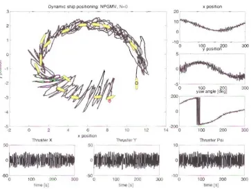
Two simulation scenarios were considered: point positioning ubject to wave motion and also

elliptical trajectory following. The nominal simulation results for the limiting case are shown in

Fig. 12 and 13. With the nominal eightings, the PGMV control p rformance is close to that of

PD

control (not shown) - this selection of weightings is thus au efu! starting point for the design.

The responses wcre intentionally made r ther oscillat ry in order to show the rapid improvcment

with increasing N - the results that follow indicate that anI a few steps are ufticient for a

Dynamic ship positioning. NPGMV, N~O x position

3-~-- ~---~----._-- 20

1

100~

""9'•.'lll

~tN"Y'''''\Ill'~

""h, , ~

100 . 200 300

Yposition

O~

5

o~-

~

1

-5 L - _ - - - _ _ , _ _.-J

-2

I 0 y1~angle [Je~ 300

-3 _l 160~

- ­

4t ~140 ~

I 120

- 5 L - - - ' - - - ' - -~---~---I1 0 0 L - - _

·2 0 2 4 6 8 10 12 0 100 200 300

x position

Thruster X Thruster Y Thruster Psi

50 - - - 50

10~,---o o o

_ _ _ _ _ _ --.-1

- 5 0 1 . - - - ­ -10

o 100 200 300 100 200 300 o 100 200 300

time [sj tlme[s] lime [s]

Fig. 12: Ship Positioning - PG MV control with N = 0

DynamiC ship positioning: NPGMV. N~O x position

- - - . ,...---,--- 2 0 · - - - ­

j

_1:~

J

_{-10 ' - - - -~--- - ­}

5

_~ 100 . 200 300

, Y posItIOn

_!

-2'

300

-3

·4 ~ 0

J

-5 .200

-2 a 2 4 6 6 10 12 14 0 100 200 300

x position

Thn/ster X Thruster Y Thruster PSI

5 0 , - - 50 10

0 a

-10 1

100 ~ 300 100 200 300 lJ 100 200 300

l,me{S] lima!sl time(S)

[image:35.612.122.494.104.383.2] [image:35.612.124.487.426.700.2]

Tuning Trials and Predictive Control: In the following modified design a lead term was included

in the control weighting to reduce high-frequency noise amplification, while the error weighting

Pe(:;-I) was modified by penalizing the frequency band corresponding to the wave motion

spectrum. This creates an inverted notch (bandpass) filter. In addition, th thrusters nonlinearities

were used to redefine the ontrol weighting as ';::Ju)== Fc~H('u) where F;.~(Z-I) is the nominal

linear control weighting, and H(u) is the thrust rs characteristic shown in Fig. 8. The inverse of H

was approximated by the expression: 1/ == 4.6078· signeT)

JiTI.

Such definition takes into account

the varying nonlinear gain of the actuators.

Simulation trials were performed for increasing values of the prediction horizon N. The

responses for N

=

3 are shown in Figur s 14 - J5, and the reduced effect of the wave disturbance

is evident when compared with Figs. 12-13. This is achieved at the expense of the more aggressive

thrusters action (responding and compensating for the wave motion), however with saturation

Dynamic sl1ip posItIOning: NPG V. N=3 x position

3

2

\ : : [ - . , ' " . . I

,L

_I

_j

-'0

L

---.l

I

a 100 y pOSItIOn.. 200 300

O~

·1

5 r - - - l

C

0

~

;;; _-It

0 C­

J

:[~

-2 r

a 100 20Q 300

yaw angle [deg]

-3r

4~

:::I~

.

120r

~ ~ I _lOa L- - - ­

-2 a 2 4 6 8 10 12 a 100 200 300

-5~--~-x position

Thruster X Thruster Y Thruster Psi

50 . - - - . , . - - - , 50 10

o a a

-50

100 200 300 a 300 100 200 300

time [s] time [51

Fig. 14: Ship Positioning - Modified PGMV control with N = 3

100 200

[image:37.612.110.507.102.401.2]

c

Dynamic ship positioning: NPGMV, N=3 x position

3~~--::~

-10 '

o 100 .. 200 300

Y position

5r--~---o

.~

</) -1

8-

o~

0>­

_ _ _ _~ _-..--J

·2 - -5

l

o 100 200 300

yaw angle [deg]

200 - ­

1

-5 L---'---'--~~ _-200

-2 0 2 4 6 8 10 12 14 0 100 200 300

x position

Thruster X Thruster Y Thruster Psi

50 10

o o

100 200 300 100 200 300

time [s1 time [s]

Fig. IS: Elliptic trajectory following - Modified NPGMV control witb N= 3

Final Remarks on the Example: Predictive can rol, when an extended prediction horizo 1 is used,

has the advantage that the control action can begin .veil before the changes in the refer nee signal

occur, thanks to the future set point knowled e. Thi behavior is particularly useful in trajectory

tracking applications and was dem nstrated for the maneuvering subclass of the DP problem.

In addition to the nonlinear lhru ter characteristics in the controller internal model, the use of a

nonlinear control w ighting allowed to compensate or nonlinearitie, , while defining the dynamic

weightint:>s to penalize specific frequency ranges led to m re effective wave disturbance rej etion.

The luning procedure was facilitated by using the existing PO controller as a starting point ror the

design. The method does of cour e have it limitation; namely, the nonlinear part of the model is

[image:38.612.95.510.101.416.2]

II. Despite th se limitations, it may be concluded that the NPGMV offers some advantages

relative to the basic NGMV design, exploiting the well-known GPe control properties, at the

expense of some additional complexity in the implementation. A generalization or this work will

involve state-dependent models and will make use of the full nonlinear model of the ship.

Concluding Remarks

There are many nonlinear predictive control strategies ba ed on ideas such as state-dependent

models, linearization around a trajectory and oth rs ([20] to [27 J). However, the aim of the

current development was to try to produce a control law which is related closely to fixed model

based control and simple to implement. The J PGMV control design problem for a state-space

system involved a multi-step predictive control cost-function and provided a method of

introducing future set-point information. The pI' dictive controls strategy described is a

dev lopment of the NGMV design method. It has the very nice property that if the system is linear

then the control reverts to the Generali 'ed PI' dictive Control design method which is well kn wn

and accepted in industry.

References

I. Cutler CR. and Ramaker B.L.. 1979. Dynamic rnatrix control - A computer control

algorithm, A.I.CH.E, 86th National Meeting, April 1979.

2. Clarke, D. W., C Montac j and P.S. Tuffs. 1987, Generalized predictive control - Part I, The

hasic algorithm, Part 2, Extensions and interpretations, Automatica, 23, 2, pp.l3 7-148.

3. Clark·, D. W., and C. Montadi. 1989, Properries of [!eneralised predictive control,

4. Richalet J., A. Rault, J.L. Testud, J. Papon 1978, Model predictive heuristic control

applications to industrial processes. Automatica, 14 pp. 4 J3-428.

5. Richalet, J., 1993, Industrial applications of model based predictive control, Automatica,

Vol. 29, 0.8, pp. 1251-1274.

6. Bitmead R., M. Gevers, and V. Wertz. 1990, Adaptive Optimal Control: The Thinking Man's

GPe. Prentice Hall.

7. Ordys, A.W., and D.W. Clarke. 1993, A state-space description for GPC controllers, Int. J.

Sy tems Science, Vol. 23, 0.2.

8. Grimble, M J, 2004, GMV control olnonlinear multivariable systems, KACC Conference

Contr I 2004, Univer ity of Bath 6-9 September.

9. Grimble, M J, 2005, Non-linear generalised minimum variance feedback, feedforward and

tracking control, Automatica, Vol. 41, pp 957-969.

10. Grimble, M J, and P Majecki, 2005, Nonlinear Generalised Minimum Variance Control

Under Actuator Saturation. IFAC World Congress, Prague, Friday 8 July, 2005.

11. Grimble, M J, 2006, Rohust industrial control, John Wiley, Chichester.

12. Grimble, M J, 200 I. Industrial control systems desi "Tn, John Wiley, Chichester.

13. Kwon W.II. and Pearson. A.E .. 1977. A modijied quadratic cost prohlem and feedback

stabilization of a linear system, JEEE Tran actions on Automatic Control, Vol. AC-22, No.

5, pp. 838-842.

14. Skjetne R, "The Maneuvering Prohlem", PhD thesis, 20 5, Faculty of Information

15 Fossen, T.1. , Sagatun S.l. and AJ. Sorensel . "Identtfication ofdynamically positioned ships",

Control Eng. Practice, Vol. 4, 0.3, pp. 369-376, 1996

16 Katcbi, M.R. Grimble MJ. and Y. Zhang,,,H robu t control design for dynamic ship

positioning", lEE Proceedings - Control Theory App!., Vol. 144, 0.2, 1997

17 Fossen T. 1., "Guidance and Control of Ocean Vehicles", John Wiley and Sons Ltd .. 1994

18 Fos 'en, T. I. and T. Perez, 2004, Marine Systems Simulator (MSS),

<www.marinecontrol.org>.

19. Press W H., Teukolsky SA., Vetterting W T., and B. P. Flannery, 2002, umerical Recipe

in c++: TheArt ofScientiticComputing, 'ambridge University press.

20. Michalska, H. and D.Q. Mayn , 1993, Robust receding horizon control of constrained non­

linear systems, IEEE Transactions on Automatic Control, 38, pp.1623-1633.

21. Kouvaritakis, B., M. Cannon and J.A. Rossiter, J999, onlinear model based pr dictive

control. Int. J Control. 72( 10), pp. 9 J9-928.

22. Lee, Y.I., B. Kouvaritakis and M. Cannon, 2003, Constrained receding horizon predictive

control for nonlinear ystems, Automatiea 38( 12), pp. 2093-2102.

23. Mayne. D.Q., J.B. Rawlings, C.V. Rao and P.O.M. Scokaert, 2000, Constrained model

predictive control: stability and optimality, AUfoma/iea 36(6), pp. 789-814.

24. Scokaert, P.O.M .. D.Q. Mayne and J.B. Rawljners, 1999, Suboptimal mod I predictive control

25. Brooms, A.C. and B. Kouvaritakis, 2000, Successive constrained optimisation and interpolation in noo- inear model based predictive control In!. J Control, 73(4), pp. 312­ 316.

26. Allgo,ver, F., and R. Findeisen, 1998. Non-linear predictive control of a distillation column, International Symposium on Non-linear Mode! Predictive Control, Ascona, Switzerland.

27. Camacho, E.F., 1993, Constrained generalized predictive control. IEEE Tran uctions on Automatic Control, 38, pp. 327-332.

28. lames. G., 1966, On the input-output stability f time-varying nonlinear feedback syst ms. part i: Conditions derived using concepts of loop gain, conicity, and passivity," IEEE Trans.