N
NO
O
NL
N
LI
IN
NE
EA
AR
R
P
PR
RE
ED
DI
IC
CT
TI
I
VE
V
E
C
CO
O
NT
N
TR
RO
OL
L
F
FO
O
R
R
M
MA
AN
NU
UF
FA
AC
CT
TU
UR
RI
IN
N
G
G
A
AN
ND
D
R
RO
O
BO
B
OT
TI
IC
C
A
AP
PP
PL
LI
IC
CA
AT
TI
IO
O
NS
N
S
PROF. MIKE J. GRIMBLE AND DR. ANDRZEJ W. ORDYS
Industrial Control Centre, University of Strathclyde, 50 George Street, Glasgow G1 1QE, UK,
[email protected], [email protected]
Abstract:
The paper discusses predictive control algorithms in the context of applications to robotics and manufacturing systems. Special features of such systems, as compared to traditional process control applications, require that the algorithms are capable of dealing with faster dynamics, more significant unstabilities and more significant contribution of non-linearities to the system performance. The paper presents the general framework for state-space design of predictive algorithms. Linear algorithms are introduced first, then, the attention moves to non-linear systems. Methods of predictive control are presented which are based on the state-dependent state space system description. Those are illustrated on examples of rather difficult mechanical systems.
Keywords: Model Based Predictive Control, Non-linear systems, State-Dependent Riccati Equations, Linear Quadratic Gaussian Control, Optimization.
1 . I N T R O D U C T I O N
It is well known that the Model Based Predictive Control (MBPC) originated in process industry where it was applied to slow processes which could be adequately described by rather crude linear models. The advent in computational algorithms and real time control hardware stimulates attempts to transfer this method to more demanding applications. In this paper we aim to present some developments in predictive control which are relevant for manufacturing and robotic applications.
The paper is organized as follows:
In section 2 we deal with linear predictive control. After introducing the notation and defining the control structure the method of incorporating the non-zero reference signal into the state-space equations is presented. Based on this, the state-space Generalized Predictive Controller (GPC) is derived and next the stability of predictive schemes is discussed. Finally, a Linear Quadratic Gaussian Predictive Controller (LQGPC) is introduced. This algorithm can improve stability by incorporating
finite horizon tuning parameters into infinite horizon optimization. Also, it proves to provide better performance than other predictive schemes, perhaps due to the fact that the values of tuning parameters which would result in instability for, say GPC, are still within stable region for LQGPC. It is important for fast mechanical systems where good tracking performance must be achieved. This algorithm can be computationally involving therefore some simplifications are presented which enable more efficient calculations of controls.
method presented in this section uses fuzzy Takagi-Sugeno models for prediction.
In section 4 we concentrate on algorithms which are inspired by the idea of global linearization for non-linear systems. The formulation of so-called state dependent state-space equations has lead to development of a technique which borrows from algorithmic solution for a standard linear quadratic problem and therefore is called State Dependent Riccati Equations (SDRE). This method is applied within the framework of predictive control for both finite horizon (GPC) and infinite horizon (LQGPC) algorithms. We notice that in the predictive schemes the future control actions within a finite horizon are predicted and available at a current time. This fact leads to improvements in defining the state-dependent system model and therefore to improvements in the accuracy of control.
Section 5 shows examples of application of the state-dependent predictive algorithms. This is a very recent research direction and the results are not conclusive yet. However, the numerical examples presented are very encouraging.
In section 6 we conclude the paper trying to predict the main future research directions and main obstacles to be overcome.
2 . L I N E A R P R E D I C T I V E C O N T R O L 2.1. Problem statement
The linear, time-invariant, discrete-time, finite-dimensional, nynu multivariable system of interest is represented in state equation form and is assumed to be stabilizable and detectable. The subsystem S1
denotes the plant model and the reference signal is assumed to be generated by the subsystem S0. A
slight generalization of the problem is to consider the inferred outputs
y ( t )h
, rather than the plant outputs {y(t)}, as being the signals to be controlled. The system model and the state-space plant equations to be considered, are therefore of the form:State :
1 1 1 1 1 1 1
x ( t ) A x ( t ) B u( t ) D ( t ) (1)
Output :
1 1 1
y ( t )C x ( t ) (2)
Observations :
1 1 1
z ( t )y ( t ) v ( t ) (3)
Inferred output :
1 1
h
y ( t )H x ( t ) (4)
and the state 1
1
n
x ( t )R , output y ( t )1 Rny, control u( t )Rnu, inferred output nh
h
y ( t )R , disturbances 1
1
q
( t ) R
and noise 1 y
n
v ( t )R . The
zero-mean, white noise signals
v ( t )1
and
1( t )
have the following covariance matrices:
1
1 1 v t 0
cov[ v ( t ),v ( )] R and
1
1 1 q t
cov[ ( t ), ( )] I
where the cross-covariances are assumed to be null. A model is required to predict the future values of the inferred output signal. From equations (1) and (4) obtain:
1 1 2 1 1
1
1 1 1 1
1 1 1 1 1
1 2
1 1 1 1 1 1 1 1
1
2
0 0
1 0
1 h
h
N h
N N
H A
y ( t )
y ( t ) H A
x ( t )
y ( t N ) H A
H B u( t )
H A B H B u( t )
u( t N )
H A B H A B H B
1 1 1
1 1 1 1 1 1
1 2
1 1 1 1 1 1 1 1 1
0 0
1 0
1
N N
H D ( t )
H A D H D ( t )
( t N )
H A D H A D H D
(5) With an obvious definition of terms this equation for the inferred outputs, may be written in the more concise form:
1 1
h
t ,N N N t ,N N t ,N
Y H x ( t ) G U N W (6)
The assumptions on the reference signal are similar to those presented by Tomizuka and co-authors [51], [53]. The reference signal {rh(t)} will be generated by the asymptotically stable linear stochastic state equation system model:
0 1 0 0
r r r r
x ( t ) A x ( t ) D ( t ) (7)
The zero-mean white-noise source
0( t )
isassumed to have the unity covariance. The desired future value of the reference signal p steps-ahead, is defined as a linear function of the current “reference state”:
0
h r r
r ( tp )H x ( t ) (8)
0 0 1
2
1
0 1 2
1
1 1
1
1 1
1 2
0 0
0 0
0
0
0 0 0 0 0
r r
r h
r h
r( p ) h
r
r r
r r
r
r( p )
x ( t ) x ( t )
x ( t ) r ( t p )
x ( t ) r ( t p )
x ( t ) r ( t )
x ( t )
A D
x ( t ) H
x ( t ) I
x ( t ) I
0( t )
(9) which may be written, with an obvious definition of terms, in the vector form:
0 1 0 0 0 0
x ( t ) A x ( t ) D ( t ) (10)
The current and future reference values can then be obtained as:
0 1
1
1 0 0 0
2 0 0 0
1 0 0 0 0
0 0 0
r h
r h
h
r( p )
h r
x ( t )
r ( t ) I
x ( t )
r ( t ) I
r ( t p ) I
x ( t )
r ( t p ) H
(11) which can be written in the form:
0 1
p p
R ( t ) H x ( t ) (12)
The N (1Np ) future set-point or reference values in the cost-function can be denoted as:
0 0 0 1
N RN p
R ( t ) H H x ( t )C x ( t ) (13)
The equations for the total system will now be obtained and these will determine the size of the Riccati equations in the control and estimation problems. Combining the state equations for the reference and the plant obtain the total augmented system as:
0 0 0 0 0
1 1 1 1 1 1
1 0 0
1 0
x ( t ) A x ( t ) D ( t )
u( t )
x ( t ) A x ( t ) B D ( t )
(14) which may be written in the more concise form:
1
X( t ) AX( t ) Bu( t ) D ( t ) (15)
The equation for the future inferred outputs to be costed in the criterion may be written in terms of the state vector X(t), using (5), as:
1 0
h
t ,N N N t ,N N t ,N
Y H X ( t ) G U N W (16)
and from the reference vector equation (13):
1 0 0
t ,N
R C X ( t ) (17)
The error signal may now be written, using these two equations, as:
1 1 1
h t ,N t ,N t ,N
E R Y
C0 HN
X( t ) G UN t ,N N WN t ,N (18)
That is, the predicted future error term that will appear in the cost-function is:
1
t ,N t ,N t ,N
E HX ( t ) GU W (19)
where
0 N
N t ,N N t ,NH C H , G G , W N W (20)
2.2. State-space GPC algorithm
The full derivation of GPC controller in state-space form may be found in [38]. Only the main points are recalled below.
The performance index to be minimized is defined as follows:
0
1 1 1
1
N Tt h h j h
j
T
h j
J r ( t j ) y ( t j ) Q r ( t j )
y ( t j ) u( t j ) R u( t j )
(21)
where E{.} denotes the unconditional expectation operator, and the error Qj and control Rj weightings can be different for future steps j.
The cost-function can be simplified by introducing the block diagonal weighting matrices
1
diag N
Q Q ,...,Q and Rdiag
R ,...,R0 N1
.The Jt term can therefore be written:
1 1
1 1
T
h h T
t t ,N t ,N t ,N t ,N t ,N t ,N
J E R Y Q R Y U RU
(22) Next, equations (18) and (19) are used. Note from (5)
that the disturbance model Wt ,N includes current and future values of the white noise disturbance signal. The vector of future predictive values of the signal
Ut,N is to be calculated at time t and cannot utilise knowledge of future disturbance signal components. Thus, ( HX ( t ) GU t ,N) and Wt ,N are statistically independent and zero mean, and from (22):
0T
t t ,N t ,N
T t ,N t ,N
J E HX ( t ) GU Q HX ( t ) GU
U RU J
(23)
0
T t ,N t ,N
J E{(W QW )}
Performing conditional expectation operation (as in standard LQG problem) the performance index, neglecting a constant (control independent) term, can be expressed as:
T
t t ,N t ,N
T t ,N t ,N
ˆ ˆ
J HX ( t ) GU Q HX ( t ) GU
U RU
(24)
where ˆX(t ) denotes the estimate of the extended state. Thus, by finding the stationary point, the vector of optimal control signals becomes:
1T T
t ,N ˆ
U G QGR G QHX (25)
Equation (25) can be represented in a more familiar form when the matrix H and the extended state X
are substituted by their appropriate definitions (20) and (14):
1
0 0
1 1
1
T T
t ,N N N N N
T T
N N N t ,N N
ˆx ( t )
U G QG R G Q C H
ˆx ( t )
ˆ
G QG R G Q R H x ( t )
(26) As predictive control is based on the receding horizon philosophy, only the first element from the vector Ut ,N is used and the optimization is performed again in the next step with (possibly) a new value of the reference signal.
2.3. Stability improvements through use the of terminal constraints or terminal cost
The state-space version of the GPC controller presented above is well know to lack guaranteed stability properties. Several authors have suggested modifications and improvements to the problem formulation which will lead to better stability of the closed loop system. A popular approach is to consider terminal constraints which could be equality constraints [9, 34], non-equality constraints [6] or terminal penalty in the cost function [1, 33]. In the latter case, if zero reference signal is assumed, the performance index (21) will change to:
1
1 1 1 1 0
1 1 1
1 1
1 1
N
T T
t j
j
T T
j N
J x ( t j ) H Q H x ( t j )
u( t j ) R u( t j ) x ( t N ) P x ( t N )
(27) where PN+1 represents the terminal cost weighting
matrix. Using the Principle of Optimality, PN+1can
be selected as the cost associated with infinite
horizon performance index, therefore guaranteeing that the solution has the same stability properties as the infinite horizon LQG problem.
2.4. Linear Quadratic Gaussian Predictive Control (LQGPC)
The approach, which we propose here is related to the terminal cost approach described earlier. The dynamic performance index to be minimized is defined as:
1
2 T
t
T t T
J E lim J
T
(28)where Jt is described by equation (21) or (22). This
new performance index (28) can be considered as the previous performance index (22) plus the terminal constraint which is an infinite horizon quadratic performance index.
To be able to take into account the dynamic nature of the problem a slight modification to the state space equation of the system (15) is made:
1 t ,N
X( t ) AX( t )U D ( t ) (29)
where the block matrix is constructed as follows:
T T
B
(30)
Therefore, equations (29) and (15) represent exactly the same dynamic system. The modification introduced in equation (29) will enable us to substitute directly the state equation into the performance index and therefore to solve the infinite horizon dynamic optimization problem.
The cost-function term Jt may be expanded using
equation (24):
T T T Tt t ,N t ,N
J E X ( t )H QHX ( t ) U ( G QG R )U
0T T T T
t ,N t ,N
U G QHX ( t ) X ( t )H QGU J
(31)
This cost term may therefore be written in the form:
0 2
t
T T T
c t ,N c t ,N c t ,N
J J
E X ( t )Q X ( t ) U R U X ( t )G U
(32)
where the weightings:
and
T T T
c c c
Q H QH , R G QGR G H QG
include the cross-product term Gc.
T T
1 T T
t ,N
U R G QG B SB G QHB SA X ( t )
(33)
where S is a steady state solution of the Riccati equation:
1 1
1
1 1
T T T T
j j j
T T T T
j j
S H QH A S A H QG A S B
R G QG B S B G QH B S A
(34)
with the terminal condition:ST1. Equations (33)
and (34) may be further simplified. Assuming that
matrix Sj is divided into four matrix blocks of appropriate dimensions:
1 2
2 3
j j
j T
j j
S S
S
S S
(35)
and using definitions of matrices as given in equations (14) and (20) obtains:
1 1 1 1 1
1 1 1 2
1 0
T T
t ,N N N
T T
N N
T T
N N
U R G QG B S B
ˆ
G QG A B S A X ( t )
B S A G Q R ( t )
(36)
and equation (34) may be split into two equations:
1 1
1 1 1
1
1 1
1 1 1 1 1 1
1 1 1 1
T T
j N N j
T T T T
N N j N N j
T T
N N j
S A H QH S A
A H QG S B R G QG B S B
G QH B S A
(37)
2 2
1 1 1 0
1
1 1
1 1 1 1 1 1
2 1 1 0
T T T
j N j
T T T T
N j N N j
T T
j N
S A H Q A S A
A H QG S B R G QG B S B
B S A G Q
(38)
2.5. Implementation to Manufacturing Systems A property of the above particular minimization problem enables the solution procedure to be simplified and made numerically efficient. First note that the vector of future controls, Ut,N can be
partitioned into those determining the control input
u(t), at time t, and the controls for
t
that willnow be denoted as Ut ,Nf . Assuming for the moment that states may be measured, this result enables u(t)
and Ut ,Nf to be computed separately. To demonstrate this result we will partition GN, Rc and Gc compatibly with the partition of Ut,N. Consider the
cost term I(t) where:
1 1 2
3 2
2
2
2 2
T T T
c t ,N c t ,N c t ,N
fT f
T T T
c c c t ,N c t ,N
f f
T T
c t ,N c t ,N
I( t ) X ( t )Q X ( t ) U R U ( t ) X ( t )G U
X Q X u R u X G u U R U
u R U X G U
(39) From (30), the dynamics of the system, involved in
the state model, do not depend upon Ut ,Nf . It follows that the optimization of the cost, depending upon
f t ,N
U is a finite dimensional problem. To obtain the gradient, with respect to Ut ,Nf we consider:
2 3 2
2 3 2
2 2
2
fT T T f
c c c
t ,N t ,N
f t ,N
fT T T
c c c
t ,N
((U R u ( t )R X ( t )G )U )
U
(U R u ( t )R X ( t )G )
(40) Setting the gradient to zero, to obtain the optimum cost, we find the vector of future controls as:
1
2 3 2
f T T
c c c
t ,N
U R ( R u( t ) G X ( t )) (41)
This provides the solution for future controls and the main problem then becomes the calculation of the feedback control at time t. The control at time t can be found by minimization of E{Jt} defined as:
0 2
T T
t c c
T c
E{ J } E{ X ( t )Q X ( t ) u ( t )R u( t ) X ( t )G u( t )} J
(42)
where
1 2 2 2
1 1 3 2 3
1 1 2 2 3
T
c c c c c
T
c c c c c
T
c c c c c
Q Q G R G ,
R R R R R ,
G G G R R
(43)
Note that when states are not available X(t) can be
replaced by the optimal estimate ˆX(t ).
Therefore, the solution of the LQGPC optimal control problem, with the multi-step cost index may be found in two stages.
Stage 1 : Vector of future controls
1
2 3 2
f T T
c c c
t ,N
U R ( R u( t ) G X ( t )) (44)
Stage 2 : Minimization in terms of current control. This minimization can be performed using polynomial description of the system as follows:
1 1
1
1
1 2
1
2 2
T
T T
c c
T t T
T T T
c c
c XX c uX
z c uu
J lim E X ( t )Q X ( t ) u ( t )R u( t )
T
X ( t )G u( t ) u ( t )G X ( t )
trace Q ( z ) G ( z )
j
dz
trace R ( z )
z
(45) The optimal control, tracking and feedback components, may be computed using:
1 1
0 N 1 1
u( t ) K ( z )R ( t ) K ( z )z ( t ) (46) where the matrix polynomials K0(z-1) and K1(z-1) are
obtained through standard minimization procedures applied to (45) and to the polynomial equivalent of the system model.
3 . N O N - L I N E A R P R E D I C T I V E C O N T R O L – A N O V E R V I E W
The development of predictive control algorithms for non-linear systems has started relatively recently. The techniques that are being used are often a direct extension of techniques for linear systems. This happens even if specific non-linear modeling methods such as neural nets or fuzzy logic are applied to prediction of future outputs. It is therefore inevitable that some sort of linearization of the system model must be performed to allow for introduction of Linear – Quadratic theory. Therefore, many researchers concentrate on defining specific conditions, which will allow linearized algorithms to work on non-linear and constrained systems. This includes the issues of stabilizability and feasibility. Another important issue is construction of efficient prediction algorithms, which would enable for fast calculation of the optimum of the performance index. A sample of different methods of non-linear predictive control is presented below.
3.1. Contractive predictive control
In this method of non-linear predictive control [28] two sampling intervals are considered. The normal sampling interval T determines the frequency of changes of the control action. The “contractive” sampling interval, which is multiplicity of the normal sampling interval: P
T determines frequency of application of the contractive constraint. The system is described by a non-linear differential equation:dx( t )
f ( x( t ),u( t ))
dt (47)
and the control action is assumed piecewise constant between sampling moments. The performance index
is a quadratic form with respect to the state, the control action and the increment in the control action:
1 1
1
k k
k k
k
k
t t
T T
k
i t t
t T
u i t
J( t ) x ( t )Qx( t )dt u ( i )Ru( i )
u ( i ) u( i )
(48)
where tk and tk+1 denote two sampling moments
distanced by the “contractive” sampling interval. Therefore, the summations in equation (48) are performed over P steps. The predictive control law is designed to minimize the above performance index subject to the state equation constraint (equation (47)), the upper and lower constraints on the control action:
min max
u u( i ) u , (49)
the constraints on the speed of changes of the control action:
max
u( i ) u
, (50)
the constraint on the horizon of the control action:
0 u u 1 1
u( i ) for i N ,N ,...,P
(51)
where Nu is the control horizon,
and finally, the “contractive” constraint:
1 1
T T
k x k k x k
x ( t )P x( t )x ( t )P x( t ) (52)
where 0 1 and Px is a positive definite matrix. The control actions within the horizon
t ,tk k1
are calculated using a non-linear numerical optimization algorithm and then applied to the system in Psampling periods. The procedure is then repeated at the time instant tk+1.
3.2. Efficient non-linear predictive control This approach was originally developed for linear systems with constraints [26]. Several extensions have been proposed to handle non-linear systems [4, 5, 27].
The underlying idea is to split the infinite control horizon
u( t ),u( t1),...
into two parts. The first part
u( t ),...,u( tM )
will be subject to system constraints and non-linear optimization may be needed to calculate it. The second part
u( tM1),...
will be assumed linear function of the system state:u( tMj )Kx( tMj ) (53)
enough by the linearized model around zero (steady state) system state:
1
x( t ) Ax( t ) Bu( t ) (54)
At the end of the first part of optimization, it is assumed that the system state will fall into a so-called invariant set that guarantees feasibility and stability thereafter. It means that a linear, stabilizing control law K will maintain the system state within the set and the set itself will be assumed ellipsoidal:
1
1
T x x : x x x
where
0
x
(55)
A semi-definite programming solver can be used to determine the maximum possible value of x which will provide the invariance and will satisfy the input constraints:
max
u( t ) Kx( t ) u
For the first M+1 moves of the control signal, it is recognized that more freedom in the control action will be needed to compensate for constraints and non-linearities. Therefore, the control law is assumed in the form:
u( t )Kx( t ) c( t ) (56)
where c(t) represents a correction or a “trim” to the control action and is used for optimization purposes. The optimal, predictive control problem can now be formulated as follows:
For a given non-linear system model:
1
x( t ) f ( x( t ),u( t ))
find a set of M values of c(t) (equation (56)) such that the quadratic performance index:
1 1 0
1
1 1 0
T T
t j t j t j t j j
M
T T T
t j t j t j t j M M M j
J x Qx u Ru
x Qx u Ru x P x
(57)
is minimized and the state xM lies in an invariant set.
The performance index (57) can be optimized numerically and, in some cases, this can be reduced to solving a linear programming task.
3.3. Fuzzy Takagi-Sugeno models in predictive control
Takagi and Sugeno proposed, [51], a type of fuzzy models suitable for the approximation of a large class of non-linear systems. This model is expressed by a set of rules Ri in the form:
1 1 1
If and and then
i i n in i i n
R : x is A x is A y f (x , ,x )
(58)
where x ,1 ,xn are the input variables of the model;
1
i in
A , , A are the fuzzy sets associated to the input variables, yi is the output of the rule i, and fi is a
function that could be linear, so that:
i 0 1 1 n
y pi p xi pin x (59)
where p ,0i ..., pni are the consequent parameters of the rule i.
Combining the values of the outputs generated by all the rules in the model, the output of the fuzzy model is given by:
1
1
M i i i
M i i
y
y
(60)
with M as the number of the rules of the fuzzy model. Also, i corresponds to the degree of satisfaction of
the rule i, defined as:
i1 ij in
i oper A , , A , , A
(61)
where “oper” is a triangular norm given by the
minimum or product operator, and ij A
is the membership degree of the input variable xj associated
with the fuzzy set Aij; for j = 1,..., n.
Takagi - Sugeno dynamic models can be used to state space description of the system:
1 1
If and … and
then 1
i i n in
i i i i
R : x (t) is A x (t) is A
x (t + )A x( t ) B u( t ) C
(62)
where x
x ,1,xn
T is the state vector of the model; Ai, Bi and Ci are the matrices of the linear models in state variables for the consequences and xiis the output vector in state variables for the rule i.
Presented below is a fuzzy predictive controller based on linearization of the Takagi-Sugeno fuzzy model [50]. For the fuzzy model given by equation (62), the equivalent time-variant linear model can be constructed:
1
where 1 M i i i
A( t ) ( t )A
, 1 M i i iB( t ) ( t )B
and1
M
i i i
C( t ) ( t )C
with i being the normalizedsatisfaction degree of the rule i.
At every sampling time, a linear model is derived by evaluating the fuzzy model premises or the satisfaction degrees. Then, a linear predictive controller is designed for the resulting linear model and, in the next sampling time, the linear model is updated.
4 . N O N - L I N E A R P R E D I C T I V E C O N T R O L W I T H S T A T E D E P E N D E N T S T A T E - S P A C E M O D E L S
This approach is based on performing a dynamic linearization around the state trajectory and applying a receding horizon strategy. There are some similarities to the non-linear algorithms presented earlier.
Only a deterministic case is considered in this part of the paper. Extension to stochastic systems would require a careful consideration of effects which non-linearities will have on probability distributions.
4.1. System representation
Assume a non-linear, discrete in the time system described by the following equations:
State:
1 1 1 1 2 1
x ( t ) f ( x ( t ))f ( x ( t )) u( t ) (64)
Inferred output:
3 1
h
y ( t )f ( x ( t )) (65)
where: f1 is a vector of size nx, f2 is a matrix
x u
( n n ), f3 is a vector of size ny.
The above system can be transformed into an alternative representation, with state-dependent state transition matrices:
1 1 1 1 1 1 1 1
1
h
x ( t ) A ( x ( t ))x ( t ) B ( x ( t ))u( t )
y ( t ) H( x ( t ))x ( t )
(66)
Where: A1 is a matrix ( nxn )x , B1=f2,H is a matrix
y x
( n n ).
Notice that the representation (66) is not unique [9], [35], in fact there is infinite number of possible transformations leading from equation (64) to (66). For instance, if f1 is expressed as:
11 1 11
1
1 1 1
x
x x x
n
n n n
f x ( t ), ,x ( t ) f
f ( x( t ))
f f x ( t ), ,x ( t )
(67)
then, the matrix A1(x1(t)) can be formed as follows:
1 11 1 1 1 diag x x n n f f
A ( x ( t ))
x x (68)
However, also other representations are possible and, indeed, may be more appropriate, especially when the state is close to zero.
We will denote: a( k ) a( x( k ))
Using this notation and the system model as in equation (66), the N steps ahead prediction of the state is given by:
1 1 1 2 1
1 1 1 2 1 1 1
1 1 1 2 1 2 1 1
1 1 1 2
1 1
1
2
1 ( t N ) ( t N ) ( t )
( t N ) ( t N ) ( t ) ( t ) ( t N ) ( t N ) ( t ) ( t )
( t N ) ( t N ) ( t N )
x( t N ) A A A x( t )
A A A B u( t )
A A A B u( t )
A B u( t N )
B u( t N )
(69) We introduce the following notation:
1 if if
n
( n ) ( n ) ( l ) ( k )
k l
a a a l n
a l n
(70)
then equation (69) can be expressed as:
1 1 0 1 1 1 1 1
1 1 1 2
1
1 1 2 1
1
1 1 1 1
2
1
N
( t j ) j
N
( t j ) ( t ) j
N
( t j ) ( t ) j
N
( t j ) ( t N ) j N
N
( t j ) ( t N ) j N
x( t N )
A x( t )
A B u( t )
A B u( t )
A B u( t N )
A B u( t N )
Define the following vectors, consisting of vector variables x1, u, yh:
1 1 1 1 1 t ,N
x ( t )
x ( t )
x ( t N )
, 1
1 t ,N
u( t )
u( t )
U
u( t N )
, 1 1 h h h t ,N h
y ( t )
y ( t )
Y
y ( t N )
(72) Then, 0 1 0 1 1 1 0 1 1 0 0 1 1 1 1 1
1 1 1 1 1
1 2
1 1
0 0
0
( t j ) j
( t j ) t ,N j
N ( t j ) j
( t j ) ( t ) j
( t j ) ( t ) ( t j ) ( t )
j j
( t j ) j
A
A
x( t )
A
A B
A B A B
A
1 1 1
1 1 1 1 1 1 2
t ,N
N N N
( t ) ( t j ) ( t ) ( t j ) ( t N )
j j N
U
B A B A B
and: 1 2 1 1 0 0 0 0 0 0 0 0
( t ) ( t ) h
t ,N t ,N
( t N )
H H Y H (73) Therefore: 1 h
t ,N N( t ,t N ) N( t ,t N ) t ,N
Y H x ( t ) G U (74)
Also, the state equation (66) can be re-written in a form that contains the vector Ut,N instead of u(t).
Direct analogy with (29) and (30) gives:
1 1 1( t ) ( t )
x ( t ) A x( t ) u( t ) (75)
4.2. State Dependent Riccati Equation technique Before progressing further with design of predictive control algorithms we mention that our method is partially inspired by the State Dependent Riccati Equation technique [10], reported to be very successful for difficult mechanical systems [35]. In this approach, the system is described by a continuous equivalent of equation (66):
1
1 1 1 1 1
dx
A ( x )x ( t ) B ( x )u( t )
dt (76)
A standard quadratic performance index:
0 0
0 1 1
T T
t t
J( t ) x ( t )Qx ( t )dt u ( t )Ru( t )
(77)is optimized. To perform optimization, an assumption is made that for a given time instant t0,
the all future values of the system parameters are to be equal to those at time t0 (one step ahead horizon
for the system parameters changes). Consequently, the algebraic state-dependent Riccati equation (SDRE) is solved, to obtain S x
1 .
1 1 1 1 1 1 1 1 1 0
T T
A x SSA x SB x R B x S Q (78) Accepting only S x
1 ST
x1 0 x1.Then, the optimal control is given by a well-known equation:
1 1
T
u( t ) R B x S x x( t ) (79)
If equation (78) could be solved analytically it would produce an analytical equation for u. However, in the normal circumstances, it is solved numerically for a given value of x1. Next, the system state is updated
and, consequently, new system parameters are obtained. This completes one iteration of the procedure.
Theorems concerning stability of SDRE are presented in [9] and [35]. In summary, if the pair
{A1(x1(t)), B1(x1(t))} is pointwise stabilizable and the
pair {H(x1(t)),A1(x1(t))} is pointwise detectable in the
linear sense for all x1 in the neighborhood of the
origin, then the system controlled by the LQ regulator (79) is locally asymptotically stable.
with six states: x
1, 2, 1, 2, 3, 4
and the tip position as the output:
xf x B x u (80)
1 tip 1 1 2 2
y k C C (81)
where,ktip,C1,C2 are constants, depending on the arm characteristics.
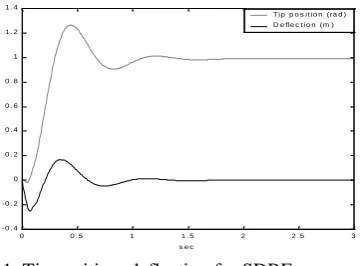
A simulated example described in this section considers that the flexible link rotates on the horizontal plane. Fig. 1 shows how the tip position changes in response to a step set-point change when the system is controlled by the SDRE method. The results compare favorably with other methods, proposed for this problem in earlier literature and are therefore highly encouraging.
0 0 . 5 1 1 . 5 2 2 . 5 3 -0 . 4
-0 . 2 0 0 . 2 0 . 4 0 . 6 0 . 8 1 1 . 2 1 . 4
s e c
[image:10.595.88.269.273.406.2]T ip p o s it io n (ra d ) D e fle c t io n (m )
Fig. 1.Tip position, deflection for SDRE
4.3. Implementation of GPC controller
Now, we move back to the design of predictive algorithm that will use state dependent state space representation. Unlike in the previous section, we will use discrete in the time system model (66) and (74). The reference model will be introduced in the same way as for the linear system (equations (10) and (13)). Therefore, the state and the “reference state” can be combined in the extended state as in equation (14):
0
0 0
1 1
1 1
0 0
1 0
1 ( t ) ( t )
A
x ( t ) x ( t )
u( t )
A B
x ( t ) x ( t )
(82)
Notice that the lower part of this system, i.e. A1(t) and
B1(t) represents the non-linear state dependent
behavior. The standard predictive control performance index will cover finite number of N steps into the future and therefore can be expressed as in (22):
1 1
1 1
T
h h T
t t ,N t ,N t ,N t ,N t ,N t ,N
J R Y Q R Y U RU
(83) The solution of the optimization problem is given by:
1
1
T
t ,N N( t ,t N ) N( t ,t N ) T
N( t ,t N ) t ,N N( t ,t N )
U G QG R
G Q R H x ( t )
(84)
The above control law is optimal for the non-linear system (82) and the quadratic performance index (83). However, the control law (84) is not causal. The matrices in the solution are functions of the future system states, which are not known when the control is calculated. Similarly to the section 4.2, a causal solution could be obtained if the analytical relationships from (82) are substituted to the prediction equation and the resulting equation is solved for u. Alternatively, one can calculate the control action iteratively as follows:
1. The current time instant is t
PART A: Initial conditions for the current time instant
2. obtain the state x(t)
3. obtain the matrices A(x(t)), B(x(t)), H(x(t))
4. assume that those matrices will remain constant for the next N steps
5. based on this (linear model) calculate the state predictions, the output predictions and the control vector Ut,N
PART B: Iterations performed within one time instant
6. substitute the calculated Ut,N into the state
equation (66) and calculate iteratively the state predictions and associated state matrices:
1 1 1 1 ( t ) ( t ) ( t )
x( t ) A , B , H
…
1 1 1
1 ( t N ) ( t N ) ( t N )
x( t N ) A , B , H
7. Calculate the output predictions and the control vector Ut,N
8. check the difference between the state predictions now and in the previous iteration step, and between the control vector Ut,N
calculated now and in the previous iteration step 9. If the difference is not small enough: go back to
6.
If the difference is small enough: end iterations (Part B)
10. Increase current time index by 1 and go to 2.
4.4. Implementation of LQGPC controller Following the reasoning presented in section 2.4 the LQGPC (dynamic performance) index will be formulated as a sum of the indices defined by (83), i.e.:
1 1 1 1
0
1 1
T T
h h
t j ,N t j ,N t j ,N t j ,N j
T
t j ,N t j ,N
J R Y Q R Y
T
U RU
Notice that in this formulation, knowledge of N future states is required to construct the state-space model. Therefore, as before, the obtained solution is not causal. However, it can be approximated by an iterative procedure similar to the one described in the section above.
As before, it is assumed that at the time instant t0 it is
possible to predict N future values of control signals and therefore N future values of states of the system. Furthermore, it is assumed that the plant parameters beyond this horizon will be constant. This assumption has no implication when using performance index (83) as the optimization is performed in one step (static optimization). However, if the performance index (85) is used, the optimization problem within the horizon T+1 will require a solution of Riccati equation backward from T+1 to 1. In the iterations of the Riccati equation the last N steps (i.e. the first N steps in time) will feature changing parameters of the system.
5 . E X A M P L E
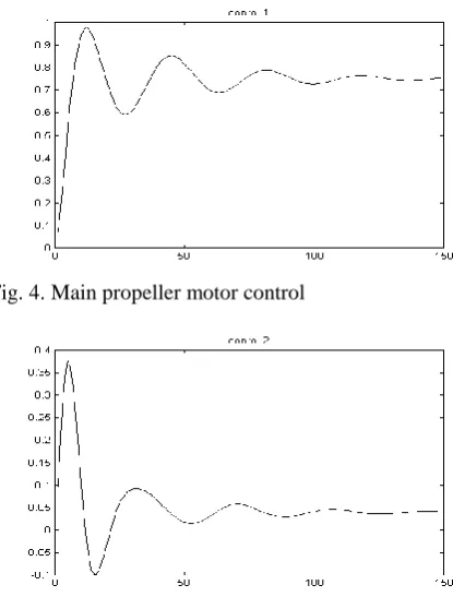
[image:11.595.314.522.56.330.2]Two examples are presented in this section. The first, which illustrates the state dependent GPC technique, is based on a simplified model of a helicopter. The model is a multidimensional naturally unstable system with two manipulated inputs and two measured outputs with significant cross-couplings. The model is described by non-linear state-space equations with two inputs, two outputs and nine states. The inputs are: the throttle valve opening for the main propeller and for the side propeller and the outputs are: elevation angle and azimuth angle.
[image:11.595.90.289.462.569.2]Fig. 2.Elevation angle with non-linear GPC
Fig. 3.Azimuth angle with non-linear GPC
Fig. 4.Main propeller motor control
Fig. 5.Side propeller motor control
For elevation angles greater than 90 degrees helicopter model is unstable. For this model, two different control algorithms have been tried. The first was based on linear GPC technique, i.e. the system non-linear equations were linearized in the current operating point and then the linear GPC solution computed and the first control applied. In the next time instant the linearization and the computations of GPC controller were repeated. This is very similar to the SDRE technique but with a finite horizon. Using this approach, all the attempts to stabilize the helicopter model failed. Then, the approach described in section 4.3 was tried and the system was successfully stabilized with the GPC non-linear controller. The results are presented in Fig. 2 to Fig. 5.
[image:11.595.94.288.607.713.2]0 0 . 5 1 1 . 5 2 2 . 5 3 -0 . 4
-0 . 2 0 0 . 2 0 . 4 0 . 6 0 . 8 1 1 . 2
n o n lin e a r g p c c o n t ro l
s e c
[image:12.595.90.275.58.204.2]D e fle c t io n (m ) T ip p o s it io n (ra d )
Fig. 6.Tip position, deflection for GPC control
0 0 . 5 1 1 . 5 2 2 . 5 3
-0 . 4 -0 . 2 0 0 . 2 0 . 4 0 . 6 0 . 8 1 1 . 2
D e fle c t io n (m ) Tip p o s it io n (ra d )
Fig. 7.Tip position, deflection for nonlinear LQGPC control.
6 . C O N C L U S I O N S
I a recent excellent tutorial session [48], Jacques Richalet, whose contribution to the field of predictive control, e.g. [49,47] is unanimously appreciated, specified 4 basic principles by which all those algorithms which pretend to be named “predictive” should be judged. Those principles are:
internal model; i.e. the model of the system is known and used internally in the control algorithm to predict the future outputs
reference trajectory, is defined for a finite number of steps into the future
structurization of manipulated variables, i.e. the control action is approximated by a combination of pre-defined functions of time
self-compensation.However, one may find out that those principles are not fully obeyed in the majority of predictive control literature. Many researchers with a background in LQG optimization wish to see the predictive control as a special case (namely finite, receding horizon) of LQG problem. Whereas the four principles listed above do not even mention optimization, only a definition of a reference trajectory.
Also, we admit that this presentation is biased by the “Linear-Quadratic optimization” thinking. However, trying to bear in mind that the Model Based Predictive Control is a more general approach, not a
special case of the LQG method, let us consider some consequences this may have on design of algorithms, especially in non-linear and/or constrained cases.
The reference trajectory:
Very often the papers on predictive control contain the sentence: without loss of generality assume zero
reference signal. This is not necessarily so easy,
especially in the real applications where the human operator or the higher level in the automatic control hierarchy would need to have a facility to change the value of the reference signal on-line while the algorithm is running. We believe that the way of describing the reference signal provided in section 2.1 addresses this problem.
Set-point and stability:
Many publications base the stability analysis on methods that assume the equilibrium point at the origin in the state space [25, 29]. For non-zero reference signal the state of the system not necessarily stabilizes at zero and in non-linear and constrained cases this will strongly affect the stability and feasibility considerations.
Structurization of manipulated variables:
This approach is now gaining popularity due to its promising features and computational advantages for non-linear systems [14, 31, 46]. Notice that standard, LQG based predictive control algorithms can provide zero steady state error for constant reference signal. For reference being a ramp function the tracking error will be constant, determined by the closed loop gain. However, when using the appropriately structured manipulated variables it is possible [47] to achieve zero steady-state error for a ramp reference function or even faster changing reference signals (e.g. quadratic function of time).
Reduced order controller:
As a consequence of structurization of manipulated variables, the order of the controller can be pre-specified at the design stage and can be lower than the dimension of the system state. The price paid for this is that the parameters of the controller will have to change from step to step [55]. However, in most of non-linear predictive algorithms even without structurization of the manipulated variables, the controller is being re-calculated in every step and still results in a high order dynamic system. Being able to reduce the order of the controller dynamics may be an attractive feature if a computational power is limited or a particular hardware imposes restrictions on the controller structure.
Acknowledgments
The authors wish to thank Mr. Alaa Eldien Shawky Mohamedy and Mr. Arkadiusz Dutka for providing the application examples and running the simulations. Comments from Mr. Baris Bulut are acknowledged.
[image:12.595.87.274.239.367.2]