Manuscript received ...; revised …; accepted … This work was partially supported by the National Natural Science Foundation of China (NSFC) Key Project No. 61332002 and by the NSFC Youth Projects No. 61502542 and No. 61300044 (Y.-J. Gong and J. Zhang are equally contributed corresponding authors, email: [email protected]; [email protected]).
X.-Y. Zhang, Y.-J. Gong, Z.-H. Zhan, W.-N. Chen, and J. Zhang are with the Key Laboratory of Machine Intelligence and Advanced Computing, Ministry of Education, China and with the Engineering Research Center of Supercomputing Engineering Software, Ministry of Education, China.
Y.-J. Gong is also with Department of Computer and Information Science, University of Macau, Macau.
Y. Li is with the School of Engineering, University of Glasgow, Glasgow G12 8QQ, U.K.
Abstract—Operating mode scheduling is crucial for the lifetime of wireless sensor networks. However, the growing scale of networks has made such a scheduling problem more and more challenging, as existing set cover and evolutionary algorithms become unable to provide satisfactory efficiency due to the curse of dimensionality. In this paper, a Kuhn-Munkres parallel genetic algorithm is developed to solve the set cover problem and is applied to lifetime maximization of large-scale wireless sensor networks. The proposed algorithm schedules the sensors into a number of disjoint complete cover sets and activates them in batch for energy conservation. It uses a divide-and-conquer strategy of dimensionality reduction, and the polynomial Kuhn-Munkres algorithm are hence adopted to splice the feasible solutions obtained in each subarea to enhance the search efficiency substantially. To further improve global efficiency, a redundant-trend sensor schedule strategy is developed. Additionally, we meliorate the evaluation function through penalizing incomplete cover sets, which speeds up convergence. Eight types of experiments are conducted on a distributed platform to test and inform the effectiveness of the proposed algorithm. The results show that it offers promising performance in terms of the convergence rate, solution quality, and success rate.
Index Terms—parallel genetic algorithm, set cover problem, large-scale wireless sensor networks, Kuhn-Munkres algorithm.
I. INTRODUCTION
IRELESS sensor networks (WSNs) have been widely used in a number of fields to satisfy various requirements, such as road traffic monitoring [1], environmental observation [2], healthcare sensing [3], and asset monitoring [4]. Typically, hundreds or even thousands of sensors, each with a series of transceivers, a battery and a micro central processing unit, are deployed in a target area. Since it is impossible to recharge or replace the battery in some scenarios, how to extend the lifetime of WSNs becomes a critical task [5].
Existing ways for lifetime enhancement are classified into five categories: operation mode control [6], data processing [7][8], sink relocation [9]-[11], topology control [12][13], and optimal routing [14]-[16]. There are various definitions of the network lifetime. In this paper, the lifetime of a WSN refers to the duration of time that the network is able to carry out its set mission. Normally, the networks can fulfill its mission if it can guarantee the specified coverage requirements by the sensors deployed, i.e., the set cover condition is satisfied [17].
As summarized in [18]-[20], the deployment methods for sensors in WSNs vary with applications, which can be categorized into deterministic deployment and random deployment. Deterministic deployment is applied to a small- or medium-scale network in a friendly sensory environment [21]-[23]. The set cover problem here can be transformed into a minimum set cover problem or its dual problem. There are some certain theoretical developments [24]-[26] and optimization algorithms [18][21] related to this field. Since this problem is NP-hard, evolutionary-computation based solvers are potentially promising because of their powerfulness in dealing with NP-hard problems. However, the optimal number of sensors cannot be known in advance, which increases the difficulty of applying an evolutionary algorithm, such as the genetic algorithm (GA). The variable length chromosome puts a great challenge to the crossover operation of GA. Nevertheless, this issue has been well solved recently by using a bi-objective GA [27].
When the environment is inaccessible or unfriendly, or the number of sensors is too large, sensors are often scattered from an aircraft or by other means of transportation, which in effect results in random deployment. In order to guarantee coverage and connectivity, the sensors are to be densely deployed in target areas. To construct an energy-efficient WSN in this case, sensors are assigned to different cover sets independent of one another [28]. Activating them in batch ensures that only one cover set is active at a time and the others are scheduled to sleep. This scientific problem is known as the Set K-cover problem [29] or Disjoint Set Covers problem [30], which is a nondeterministic polynomial complete (NP) problem and hence its optimization is NP-hard.
A common objective of solving the Set K-cover problem is to maximize the lifetime of the WSN, but they differ slightly in terms of coverage constraints. In [31], sensors are aimed to be scheduled into K disjoint sets while guaranteeing that the coverage ratio of each set is as high as possible by modeling
Kuhn-Munkres Parallel Genetic Algorithm for
the Set Cover Problem and Its Application to
Large-Scale Wireless Sensor Networks
Xin-Yuan Zhang, Yue-Jiao Gong, Member, IEEE, Zhi-Hui Zhan, Member, IEEE, Wei-Neng Chen, Member, IEEE, Yun Li, Member, IEEE, and Jun Zhang, Senior Member, IEEE
R
z1
z2
s
[image:2.612.411.475.54.114.2]s
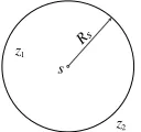
Fig. 1. Boolean Disk model. Considering two points z1 and z2 in the target
area, we have f (D(s, z1)) = 1 and f (D(s, z2)) = 0.
the Set K-cover problem as an N-person card game, and solutions are obtained after a gaming process. A heuristic
method, termed the Most Constrained-Minimally
Constraining Covering (MCMCC), is proposed in [29]. The essence of MCMCC is to minimize the coverage of sparsely covered areas within one cover set. It requires that each cover set is able to cover the target area completely. We focus on complete cover sets in this paper.
Owing to their success in solving nondeterministic polynomial problems, GAs [32]-[34] and other evolutionary algorithms (EAs) [35]-[37] have been applied to the lifetime problem in WSNs recently. Lai et al. [38] propose a GA for maximum disjoint set covers (GAMDSC), which applies a scattering operator to the EA offspring to keep critical sensors from joining the same cover set. Hu et al. [39] propose a schedule transition hybridized genetic algorithm (STHGA), which adopts a forward encoding scheme for chromosomes and utilizes redundancy information via designing a series of transition operations. Ant-colony optimization for maximizing the number of connected cover (ACO-MNCC) is proposed in [40], which maximizes the lifetime of heterogeneous WSNs. These algorithms are shown competitive in solving small to medium sized WSNs. However, the performance of existing methods decreases substantially when dealing with a large-scale Set K-coverSet problem.
To improve set cover efficiency and large-scale WSN performance over existing algorithms, a Kuhn-Munkres scheduled parallel GA (KMSPGA) is developed in this paper, so as to provide the following features and benefits:
A divide-and-conquer strategy to achieve dimensionality
reduction in a simple but effective way and solve the small-scale Set K-cover problem separately in each subarea;
The merging of local feasible solution is modeled as a
Maximum Weight Perfect Matching (MWPM) problem such that Kuhn-Munkres (KM) algorithm [41][42] is applicable;
A redundant-trend sensor schedule strategy (RTSS) to
further improve global search efficiency, which is easier to implement than the existing auxiliary schedule strategies [39], and
A modified fitness index by introducing a coverage
inadequate penalty to guide convergence better.
The rest of this paper is organized as follows. In Section II, we describe the Set K-cover problem for WSNs, with assumptions and definitions given. In Section III, we develop KMSPGA in detail. This parallel genetic algorithm is comprehensively tested for performance through simulations in Section IV. Finally, conclusions are drawn in Section V.
II. PROBLEM FORMULATION
A. Sensor Model
In this section, we introduce the sensor model adopted in our algorithm, which is crucial for the coverage, connectivity, and energy consumption.
A sensor coverage model is an abstract concept to measure the sensing capability and to quantify how well a sensor can monitor the occurrence of events within its sensing range. Various models have been proposed, such as the Boolean sector coverage model and the attenuated disk coverage model [43]. Comparisons of existing models are made in [44]-[46].
In this paper, we adopt the Boolean disk model because of its concise definition and wide applicability [19][43], which is illustrated in Fig. 1. This model ignores the dependency of environmental conditions. A point in the space of the target area is considered to be covered only if it is within the range of at least one sensor. A coverage function is formalized as:
1, if ( , )
( ( , )) 0,
s
D s z R
f D s z
otherwise
(1)
2 2
( , ) ( x x) ( y y)
D s z s z s z (2)
where s = (sx, sy) is the central coordinate of a sensor and (zx, zy)
is the coordinate of point z in a 2-dimensional space, Rs is the
sensing radius and D(s, z) calculates the Euclidean distance between s and z. Once a point is covered by a sensor, the coverage function value is 1, otherwise, it is 0. In [47], a geometric analysis of the relationship between coverage and connectivity is provided, showing that the connectivity can be guaranteed inherently if 1) coverage is satisfied and 2) the communication range of sensors is no less than twice of the sensing range. Afterwards, many related publications for solving the Set K-cover problems are based on this proof [31][39] that they use the sensors with communication range at least twice than the sensing range and consider the coverage constraint only. In this paper, we also make such an assumption and meet the connectivity constraint by satisfying the coverage constraint.
E1
E2
E3
E4
E5
E6
E7
E8
(a) (b)
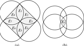
[image:3.612.376.514.59.134.2]Ex
Fig. 2. Notion of an element and a K-covered element. (a) The shaped area is divided into eight elements E1, E2, …, E8, where four elements are covered by
two sensors and the remaining four by one only. (b) Element Ex is called
K-covered, if it is covered by K sensors, in which case K = 4.
1
2
3 4
5 6
7
8 9
10 11 12
13 14
15
[image:3.612.388.495.181.249.2]16
Fig. 3. Elements E1, E3, E6, E8, and E15 are called critical elements, as they are
covered by the minimum number of sensors. there is still room for KMSPGA to adapt this framework to
fitting new forms of energy constraints. B. Set K-Cover Problem
In this paper, we focus on maximizing the lifetime of a large-scale WSN using a static optimization strategy. The proposed KMSPGA is an off-line algorithm that pre-calculates K disjoint complete cover sets at a time. By alternatively activating the K cover sets in batch, the lifetime of the WSN can be K times larger than the lifetime of a single cover set. Hence, maximizing the lifetime of the WSN is equivalent to finding the maximum disjoint complete cove sets.
We consider the Set K-cover problem a scheduling problem. For a positive integer K, sensors are judiciously scheduled into K disjoint cover sets such that each cover set is able to meet the coverage requirement. In this paper, we focus on a complete coverage. The premise of finding K disjoint complete cover sets is that every element of the target area is covered by at least K sensors. Sufficiency of this premise is proven in the following of this subsection. Fig. 2 illustrates the concept of an element and a K-covered element. In Fig. 2 (a), the grey square area is divided into eight elements. Element Ex in Fig. 2 (b) is
covered by four sensors; hence it is called 4-covered.
Without loss of generality, assume that a target area Γ is a rectangle and that N sensors S1, S2, …, SN are randomly
deployed in Γ. A constraint of the coverage requirements is a complete coverage. Given a positive number K, sensors are scheduled into K cover sets C = {C1, C2, …, CK}. For each
cover set Ci (i= {1, 2, …, K}), if every element of Γ is covered
by at least one sensor in Ci, then C would be considered as a
feasible solution of the Set K-cover problem. The Set K-cover problem can be formalized as:
( ) k i k S C E S
(3)
1 K
i i
C S
(4)
, , , {1, 2,..., }
i j
C C i j i j K (5)
where E(Sk) represents the element sensed by sensor Sk, k is the
sensor index, S is the collection of sensors. Assume that the target area is partitioned into M elements E1, E2, …, EM. To
make a clear explanation of how to calculate the upper bound of K, we first give the following proposition and its proof:
Proposition 1: The prerequisite of finding K disjoint cover sets is that each element is covered by at least K sensors.
Proof: Assume that Eτ is covered by Q sensors SCτ = {Sτ,1,
Sτ,2, …, Sτ,Q}, where SCτ is the collection of sensors covering
element Eτ. There still exist K disjoint complete cover sets with
Q < K.
Let C be a feasible solution of the Set K-cover problem. Then, we have |C| = K. Considering the same element Eτ in the
assumption, Eτ is expected to be covered in each Ci ∈ C
according to (3). Then, K cover sets are considered as K covering tasks, and we have Q sensors that can perform this task. Then, K tasks are assigned to Q sensors. Since we have |C| = K > |SCτ| = Q, there exist cover sets Cp, Cq ∈C, and
sensor Sτ,m∈SCτ (m∈ {1, 2, …, Q}) satisfying Sτ,m∈Cp∩Cq
according to the drawer principle, and therefore it contradicts
(5). In conclusion, the assumption is invalid and hence the proposition is proven to be tenable.
In order to better explain how to estimate the upper limit of K, the notion of critical element and critical sensor is introduced as follows. The target area is partitioned into a number of elements by thousands of densely deployed sensors. An element covered by the minimum number of sensors is called a ‘critical element’ and the corresponding sensors ‘critical sensors’. Fig. 3 illustrates critical elements and critical sensors, where six sensors divide the rectangular area into sixteen elements E1-E16. Being covered by one sensor only, elements E1, E3, E6, E8, and E15 are critical elements.
Let Ec be a critical element. Assume that the number of
sensors covering Ec is Û. According to Proposition 1, we can
at most find Û disjoint complete cover sets only if the Û critical sensors are chosen in Û disjoint cover sets which guarantee that Ec is covered by every cover set, and therefore
Û is regarded as the upper limit of K. C. Critical Parameters
In this subsection, we discuss some critical parameters related to a large-scale WSN. A redundant rate represents the density of sensors deployed in the target area. The redundant rate in the 2D ideal plane model is computed as (6) according to [39], where area(Γ) is the area of Γ and N is the number of sensors.
2
ˆU ( )
s
N R
area
(6)
It is difficult to compute the coverage ratio of Γ accurately when applying the Boolean disk model. For this reason, we divide the target area into T smaller square grids (g1, g2, …, gT),
T being computed as (7), where d is the width of the grid. A coverage ratio is defined as (8), where Ng(Si) represents the
collection of grids covered by sensor Si and |Ng(Si)| is the
number of grids in Ng(Si). Equation (9) indicates that a grid
belongs to no more than one collection in case of a repeat count.
2
( ) area T
d
Algorithm 1 Preprocessing of choosing a proper grid width 1: Procedure WIDTHCHOOSE {d1,…,dΨ}
2: d ← d1 ; 3: Compute Û1 ; 4: fori = Ψ → 2 do
5: d ← di ;
6: Compute Ûi
7: if Ûi = Û1 then
8: d ← di ;
9: break ; 10: end if
11: end for
12: returnd ; 13: end procedure
[image:4.612.328.563.52.134.2](a) (b) (c)
Fig. 4. Calculation of the coverage ratio. (a) The light grey grids are covered while the black one is not covered because one of its vertices is beyond the sensing range of the sensor. (b) The black grid is covered by two sensors Sp
and Sq, but only belongs to either of Ng (Si), i∈ {p, q}, in the case of a repeat
count. (c) The coverage ratio is 11/25 = 0.44.
[image:4.612.335.563.305.555.2](a) (b)
Fig. 5. An example to show how the grid width influences the computation of the coverage ratio. (a) The grey grid is regarded as uncovered due to the coverage criteria. (b) The grey grid becomes covered by either of the two sensors after the grid width is shortened.
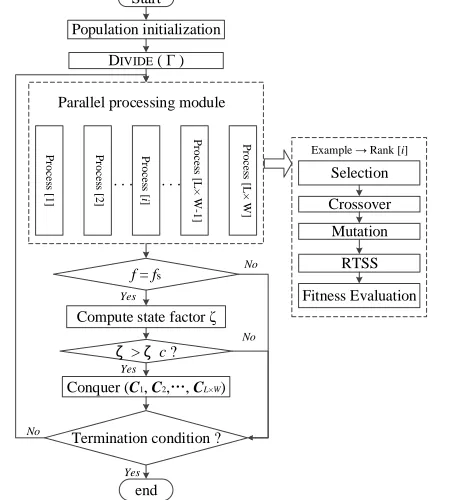
Start
end Population initialization
DIVIDE ( Γ )
Fitness Evaluation Crossover
Mutation
RTSS
f = fs
. . .
No
Compute state factor ζ
Yes
ζ > ζ c ?
No
Conquer (C1, C2,, CL×W)
Example Rank [i]
Termination condition ?
No
Yes
Parallel processing module
. . .
P
roc
es
s
[L
×
W
]
P
roc
e
ss
[1
]
P
roc
es
s
[L
×
W
-1
]
P
roc
es
s
[
i
]
P
roc
e
ss
[2
]
Selection
[image:4.612.318.563.574.738.2]Yes
Fig. 6. Flowchart of the Kuhn-Munkres parallel GA framework.
1
1
| ( ) |
N
g i
i
N S
T
(8)( ) ( ) , , , {1,2,..., }
g i g j
N S N S i j i j N (9)
The coverage criteria stipulates that grid gj is covered by
sensor Si only if all its four vertices are within the sensing
range of Si. Fig. 4 shows how to calculate the coverage ratio.
This calculation method is widely used to estimate the coverage ratio [39][40]. However, the grid width can influence the computation of the coverage ratio in terms of computational complexity and accuracy. Fig. 5 gives an example to explain this special case, where the grey grid is apparently covered by the WSN. Unfortunately, it is regarded as uncovered due to the above coverage criteria whether a grid is covered. If the width of this grid is halved, two resultant grids become covered. However, the calculation of the coverage ratio is of an O(N×T) computational complexity. A shorter width means a higher computational complexity according to (7).
In our work, we adopt a simple strategy to determine the grid width in a preprocessing step. Given Ψ kinds of di (i= {1,
2, …, Ψ}, di < di+1) in the process of estimating the upper limit
of K, we choose the smallest d1 first to obtain an exact value Û1, because d1 is small enough to guarantee accuracy. Then di (i =
{2, 3, …, Ψ}) is adopted to work out Ûi in sequence. The
largest di (ensuring Ûi = Û1) is used for calculating the
coverage ratio. Algorithm 1 presents a set of pseudocode of this preprocess of choosing a proper grid width. In this paper, we adopt 5 kinds of grid widths: (d1, d2, d3, d4, d5) = (0.625, 0.78125, 1, 1.25, 1.5625).
III. PROPOSED PARALLEL GENETIC ALGORITHM A. Kuhn-Munkres Parallel Genetic Approach
KMSPGA is designed on a divide-and-conquer strategy, and the polynomial KM algorithm is adopted to splice the feasible solutions obtained in each subarea. The framework of KMSPGA is shown in Fig. 6. In the first step, we uniformly divide the target area into a number of subareas and encode them. Assuming that the number of sensors within subarea Ai
is Ni, it satisfies:
1 L W
i i
N N
(10)where L and W denote the number of partitions along horizontal and vertical directions respectively, and hence L × W denotes the number of subareas obtained. Therefore, the Set K-cover problem size of subarea Ai is whittled down to Ni.
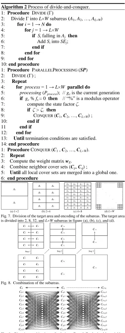
Algorithm 2 Process of divide-and-conquer. 1: Procedure DIVIDE (Γ)
2: Divide Γ into L×W subareas (A1, A2, …, AL×W)
3: for i = 1 → Ndo
4: forj = 1 → L×W
5: if Si falling in Aj then
6: Add Si into SEj;
7: endif
8: endfor
9: endfor
10: end procedure
1: Procedure PARALLELPROCESSING (SP) 2: DIVIDE (Γ);
3: Repeat
4: for process = 1 → L×W paralleldo
5: processing (Pprocess); // gc is the current generation
6: if gc % fs = 0 then // “%” is a modulus operator 7: compute the state factor ζ.
8: if ζ > ζc then
9: CONQUER (C1, C2, …, CL×W) ;
10: endif
11 end if
12: end for
13: Until termination conditions are satisfied. 14: endprocedure
1: Procedure CONQUER (C1 ,C2, …, CL×W).
2: Repeat
3: Compute the weight matrix wE.
4: Combine neighbor cover sets (Cp, Cq) ;
5: Until all local cover sets are merged into a global one. 6: endprocedure
A1 A7 A5 A3 A1 A8 A6 A4 A2 A29 A25 A21 A17 A13 A9 A5 A1 A30 A26 A22 A18 A14 A10 A6 A2 A31 A27 A23 A19 A15 A11 A7 A3 A32 A28 A24 A20 A16 A12 A8
A4 . . . .
. . . . . . . . . . . . . . . . .
(a) 1´2 (b) 2´4 (c) 4´8 (d) L´W
A2
Fig. 7. Division of the target area and encoding of the subareas. The target area is divided into 2, 8, 32, and L×W subareas in figure (a), (b), (c), and (d).
C7 C5 C3 C1 C8 C6 C4 C2 C7-8 C5-6 C3-4 C1-2 C7 C5 C3 C1 C8 C6 C4 C2 C1-4 C5-8 C1-4 C5-8 C1-8
Step 1 Step 2 Step 3
Fig. 8. Combination of the subareas.
Cp,1
Cp,2
Cp,3
Cp,4
Cp,5
Cp,6
Cp,7
Cp,8
Cp,9
Cp,10
Cq,1
Cq,2
Cq,3
Cq,4
Cq,5
Cq,6
Cq,7
Cq,8
Cq,9
Cq,10
Cp-q,1
Cp-q,2
Cp-q,3
Cp-q,4
Cp-q,5
Cp-q,6
Cp-q,7
Cp-q,8
Cp-q,9
Cp-q,10
[image:5.612.313.565.45.717.2]Cp Cq Cp-q
Fig. 9. Bipartite combinations of solutions Cp and Cq obtained by neighbor
sub-populations, such that the Kuhn-Munkres algorithm can be applied. processes and, afterwards, all the processes of KMSPGA
terminate. Pseudocode of this divide-and-conquer strategy is given in Algorithm 2.
Divide() contains two steps. Firstly, the target area Γ is uniformly partitioned into L×W subareas A = (A1, A2, …, AL×W).
Fig. 7 gives four examples where Γ is divided into 2, 8, 32, and L×W subareas in Fig. 7 (a), (b), (c), and (d), respectively. Then, the centers of all sensors are traversed to obtain a classification SE = {SE1, SE2, …, SEL×W}, where SEi is the collection of
sensors falling in subarea Ai. Every sensor within SEi satisfies
that its central coordinate (sx, sy) ∈ Ai (k = {1, 2, …, Ni}).
Additionally, if the center of a sensor falls on the boundaries of two or more subareas, it will be randomly scheduled into any one of the subareas. In order to keep the concision of KMSPGA, we adopt a uniform partition here instead of other ways such as clustering techniques. Besides, the uniform partition is convenient for the following combination operation.
In the parallel processing module, each process evolves a sub-population to obtain a feasible solution. The collection of sub-populations is formulized as SP = (SP1, SP2, …, SPL×W).
Each sub-population size is Np. They are evolved
independently through a selection, crossover, mutation, and RTSS operation in processing(). We estimate the state of each sub-population through periodically sampling the information of the best individual at a sampling frequency fs. A state factor ζ is computed as follows:
1 1 ˆU L W i i U
(11)where Ui is the number of disjoint complete cover sets
obtained by the best individual of SPi. Since Ui ≤ Û ( i = 0,
1, …, L×W), we have ζ ≤ L×W. Therefore, the upper limit of the threshold value, ζc, is set to L×W–1. The value of ζ
determines whether the KM combination operation will be applied. The independent evolution process will be terminated until ζ reaches ζc. Therefore, instead of performing the KM
operation every generation, the execution timing of KM is adaptively adjusted based on the state factor. This way, the effectiveness of the operation is improved, and hence the computational cost is substantially reduced. The threshold ζc
determines the frequency of performing the KM operation (merging the local feasible solutions) and then checking for the termination condition. This procedure however does not affect the main evolution process of solutions to much extent. Thus, different settings of ζc will not change the output solution
quality of the proposed algorithm, but only influence the execution time. The standard uniform crossover and uniform mutation are adopted in the evolutionary process. RTSS is conducted right after mutation, and before fitness evaluation, which is introduced in detail in Subsection D. The tournament selection is adopted because of its efficiency, with a tournament size Ts.
Conquer() is a combination operation in order to merge the feasible local solutions C = (C1, C2, …, CL×W)T, Ci = (Ci,1,
Ci,2, …, Ci,Û). Ci is the best solution of the small-scale Set
K-cover in subarea Ai. Fig. 8 shows an example of this merging
X x x x x x x x x
4 1 3 2 3 2 4 1
S ,S S ,S S ,S S ,S
{ C }
=
C =
1 2 3 4 5 6 7 8
2 8 4 6 3 5 1 7 1 C2 C3 C4
X
Fig. 10. Representation of chromosome. C is an equivalent way of representing a chromosome, where genes of the same value form a cover set.
Algorithm 3 Fitness evaluation
SFk: a flag variable in case of repeat count.
RFi: a flag variable representing whether Si is redundant.
1: Procedure CHROMOSOMEEVALUATION (x1,…,xN)
2: for i = 1 → Ndo
3: SFi ← 0;
4: RFi ← true; // Si is redundant if RFi is true
5: end for
6: for i = 1 → Tdo
7: for j = 1 → Ndo
8: k ← xj ;
9: if giNg(Sj) and SFk = 0 then
10: CNk ← CNk+1 ;
11: SFk ← 1;
12: RFj ← false;
13: end if ; 14: endfor
15: endfor
16: f ← 0;
17: for i = 1 → Û do
18: δi ←CNi∙T-1 ;
19: f ← f +δi∙P(δi) ;
20: endfor
21: endprocedure
to find a best combination Cp-q for each dimension ofCp and Cq
ensuring that the coverage ratio summation of Cp-q,k is maximal.
The total number of matching combinations is Û!. As shown in Fig. 9, given Û = 10, we have 10! kinds of matching ways of Cp and Cq. This combination problem can be modeled as a
MWPM problem in graph theory, which can now be solved using the KM algorithm.
In the literature, KM algorithm has been successfully applied to a number of fields, such as allocation of vehicle-to-infrastructure and vehicle-to- vehicle links [48], group role assignment [49], and user grouping for grouped OFDM-IDMA [50].Given a bipartite graph G = (V, E) and weight function w(e), MWPM aims at finding a perfect matching of maximum weight. The weight of the matching M is formulized as (12). Cover sets (Ci,1, Ci,2, …, Ci,Û) are
considered as the vertices of G (i ∈ {p, q}). Weight wi,j of edge
e between Cp,i and Cq,j is computed as (13), where
|Ng(Cp,i∪Cq,j)| represents the number of grids covered by the
sensors within Cp,i and Cq,j, and |Ng (Ap∪Aq)| is the number of
grids covered within Ap and Aq. Then, the weight matrix WE is
represented as (14). KM combination is constantly conducted until all local solutions are totally combined into a global solution.
( ) ( )
k k
e M
w M
w e (12), ,
,
| ( ) |
| ( ) |
g p i q j
i j
g p q
N C C
w
N A A
(13)
ˆ
1,1 1,U
ˆ ˆ ˆ
U,1 U,U
w w
w w
E
W (14)
B. Chromosome Representation
In this subsection, we describe the chromosome representation in KMSPGA. We compute the value of Û in the whole target area. It is worth mentioning that even if we divided the target area into subareas, we still have to ensure that the whole target area can be covered by Û complete cover sets. Therefore, Û is also the upper limit of the number of complete cover sets for each subarea, then, sub populations
SP1, SP2, …, SPL×W share the same Û. Taking Population SPk
as an example, each chromosome is encoded as X= (x1, x2, …, xn), where xi represents the batch number of sensor i, and n is
the number of sensors falling in Ak(n = Nk). Since there is at
most Û batches, we have xi∈ {1, 2, …, Û}.
For chromosome X, sensors with same batch number are chosen to a same cover set. Therefore, X is transformed into CX
= (C1, C2, …, CÛ), which is a candidate solution of Set K-cover
problem. Fig. 10 gives an example of chromosome representation and shows the relationship between X and CX,
where n is eight and Û is four. On the contrary, X can be easily transformed from CX. Therefore, X and CX are equivalent on
representing an individual. In the remainder of this section, we adopt the CX structure in representing a chromosome because
this form is more convenient for introducing and descripting the operations of KMSPGA while X is adopted in the practical implementation of KMSPGA.
C. Improved Fitness Index
In STHGA [39], the evaluation function is defined as (15), where δi represents the coverage ratio of cover set Ci. The
computation of δi is shown in (16), where the value of δi,k is 1 if
grid k is covered by Ci. The value of δi (i ∈ {1, 2, …, Û-1}) is 1
in STHGA because of the forward encoding scheme. The evaluation function of GAMDSC [38] is shown in (18), where fB represents the number of disjoint complete cover sets and ⌊x⌋
denotes the floor of x.
ˆ
1
1 U
A i
i
f
T
(15)1
( )
, 1 T L W
i i k
k
L W T
(16),
1, 0,
i i j
if grid j is covered by C otherwise
(17)
ˆ
1 U
B i
i
f
(18)In order to improve the convergence rate, we adopt a penalty function P(δi) of (19), where λ is the penalty
[image:6.612.319.568.51.329.2](a) (b) (c)
Fig. 11. Illustration of a redundant-trend sensor, with a redundant state uncertain after crossover and mutation operations. (a) Since the area covered by this sensor has already been covered by other sensors in the same cover set, the grey sensor is considered to be a redundant one. Figure (b) and (c) show two situations of redundant state of the grey sensor after the crossover and mutation operations. The grey sensor is redundant in (b) while it is no longer redundant in (c).
S2,1
S2,2
S2,7
S2,5
S2,6
S2,3
S2,4
S3,1
S3,3
S3,2
S3,5
S3,4
S4,6
S4,1
S4,2
S4,4
S4,3
S6,1
S6,4
S6,2
S6,5
S4,5
S5,1 S5,2
S5,4 S5,3
S1,1
S1,2 S1,3
S6,1
S6,1
S2,7 S1,3
S3,4
S5,4
C
C
C
C
C
C
C
1 2 3 4 5 6
Fig. 12. Redundant-trend sensors transition between disjoint cover sets, where grey sensors are redundant-trend sensors. Different cover sets are represented
by different polygons, such as the triangle representing cover set C1.
TABLE I
THE PARAMETER SETTING OF KMSPGA
Parameter Description Value
Ψ Number of grid width classification. 5
λ Penalty coefficient in cost evaluation. 0.2
L Number of partitions along horizontal direction. {2,4}
W Number of partitions along vertical direction. {2,4,8}
fs Sampling frequency. 3000
Pc Crossover probability. 0.6
Pm Mutation probability. 0.001
Nc Number of candidates in RTSS. [3-1Û]
Np Sub-population size. 15
Ts Tournament size 5
ζc
Threshold of the state factor with 2×2 partitions. 3.0 Threshold of the state factor with 2×4 partitions. 7.0 Threshold of the state factor with 4×4 partitions. 15.0 Threshold of the state factor with 4×8 partitions. 30.0 eliminated more easily than those with more complete cover
sets. Algorithm 3 shows the pseudocode of the fitness evaluation in KMSPGA.
1, 1
( ) ,
i i
if d = P
otherwise
(19)
ˆU
1
( )
i i
i
f P
(20)D. Redundant-Trend Sensors Schedule Operation
In RTSS, the redundant information is indirectly utilized in order to improve search efficiency. The redundant information is collected in the fitness evaluation process. In Algorithm3, steps 2 to 15 give this collection process. As can be noted from the pseudocode, the collection process is embedded in the fitness evaluation in case of increasing computational complexity. Note that after collecting the redundant information, RTSS is not applied directly after the fitness evaluation, but, as introduced in subsection A, it is performed after crossover and mutation operations, the landscape of the chromosome may change. Thus, the redundant information utilized in RTSS is hysteretic.
Considering that Sk is a member of Cj, whether Sk is
redundant for Cj depending on its contributions to Cj. Sk is
considered to be redundant only if it has no contributions to Cj,
which is judged in the fitness evaluation. However, Sk may not
still be redundant, because crossover and mutation operations may change the members of Cj. Therefore, Sk is called
redundant-trend sensors in RTSS due to this uncertainty of the redundant state. Fig. 11 shows an example of this uncertainty. The grey sensor is considered to be redundant after the fitness evaluation operation. However, it is uncertain whether it is still redundant after crossover or mutation.
The process of RTSS is described as follows. Suppose that the cover set is C = {C1, C2, …, CÛ}. Firstly, we traverse the redundant information of the sensors in Ci. Assuming Si,k is the
kth member of Ci, if Si,k is judged to be redundant for Ci in
Algorithm 3, we then consider it a redundant-trend sensor in RTSS. A cover set Cm (m ∈ {1, 2, …, Û}) will receive Si,k
through a tournament selection, where Nc candidates are
randomly selected and the one with the lowest coverage ratio is chosen to receive Si,k as one of its members. Fig. 12
illustrates this schedule strategy between disjoint cover sets. In Fig. 12, different polygons represent different cover sets, the grey sensors are redundant-trend sensors, and the direction of arrow represents the schedule direction. RTSS has twofold functions. It helps enhance the coverage ratio through the schedule strategy if the redundant-trend sensor is actually a redundant one. However, if the redundant sensor is no longer redundant for the current cover set, the scheduling operation becomes a disturbance for the population. This kind of stochastic disturbance enriches the diversity of the population.
IV. EXPERIMENTAL RESULTS
A. Experimental Setup
In this section, experiments are conducted to ascertain the performance of KMSPGA. In Subsection B, we compare KMSPGA with the state-of-the-art algorithms. MCMCC, GAMDSC, and STHGA are serial algorithms which perform well in solving the Set K-cover problem. The experiments and comparisons are used to verify the effectiveness of our proposed KMSPGA algorithm for lifetime maximization of large-scale WSNs. In Subsection C, we compare KMSPGA with a traditional pure parallel genetic algorithm (PGA). Further, the performance of the PGA embedding only RTSS (SPGA) or KM combination (KMPGA) are also tested in order to study the effectiveness of the two operations. Experiments in Subsection D and E are designed to evaluate the robustness of KMSPGA with different partitions and the redundant rates. In Subsection F, we conduct parameter investigation and give their suggested values. Finally, experiments in Subsections G-I are conducted with new and different testing scenarios to further verify the performance of KMSPGA.
[image:7.612.315.566.584.738.2] [image:7.612.79.261.600.706.2](a) (b)
0 10000 20000 30000 40000
0 50 100 150 200 250
Me
an
U
Mean FEs KMSPGA
STHGA
GAMDSC
0 20000 40000 60000 80000
0 50 100 150 200
Me
an
U
Mean FEs
KMSPGA
STHGA
[image:8.612.48.564.67.205.2]GAMDSC
Fig. 13. Convergence curves of the compared algorithms. (a) I3-2. (b) I6-1. 64-bit operating system. The parallel programming practice
uses the Message Passing Interface (MPI). Table I shows the parameter settings. Pc and Pm, the constant crossover and
mutation rates, are set as Pc = 0.6 and Pm = 0.001, respectively.
The value of λ determines the degree of punishment for the individuals with incomplete cover sets. In all of the test instances, we adopt λ = 0.2 as default value. Nc, the number of
candidates in RTSS, is empirically setting to 3-1Û. Sample frequency fs is set to 3000 function evaluations (FEs). In
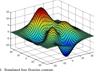
Subsections B-H, Γ is a 50×50 square area, and in Subsection I, Γ is a 3-D surface. PL×W denotes the partition way of Γ. ζc is set
to 3.0, 7.0, 15.0, and 30.0 for P2×2, P2×4, P4×4, and P4×8, respectively. Thirty trials are performed for each instance and the results are averaged over the trials. A two-tailed t-test of the null hypothesis is conducted in Subsections B, G, H, and I. The null hypothesis will be rejected if p-value is smaller than the significance level α = 0.05.
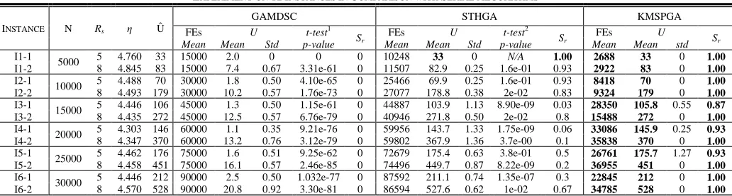
B. Comparison with State-of-the-Art Serial Algorithms We conduct experiments on 12 instances to verify the performance of KMSPGA in comparison with the serial algorithms: MCMCC, GAMDSC, and STHGA. P2×4 is adopted in this subsection.
The experimental results are listed in Table II. Mean and Std are the mean quality and standard deviation. Sr is the success
rate. The best solutions are marked in bold. KMSPGA outperforms the other algorithms in terms of the convergence rate and solution quality. Furthermore, KMSPGA produces significant increases both in the convergence rate and in the success rate in the higher dimensional space. The success rate of instances I1-1, I1-2, I2-1, I2-2, I3-2, I4-2, I5-2, I6-1, and I6-2 reach 1.00. The mean FEs is far less than the serial algorithms. MCMCC is not available because it took an unacceptable time before termination. The worst runtime of MCMCC is O(N2) [39], where N is the number of sensors. This heuristic method performs efficiently when the number of sensors is small or medium. However, the computational complexity of MCMCC becomes so high in terms of large-scale WSNs that it fails to work out a feasible solution in an acceptable time, i.e., I2-1, a single run of MCMCC exceeds eight hours. GAMDSC is another genetic algorithm used in this experiment. Since GAMDSC lacks an efficient search strategy to handle such a large number of sensors, solutions obtained by GAMDSC are fewer than Û. STHGA possesses high quality of solutions in the low-dimensional spaces when
the number of sensors is less than 5000. The complicated local search operations help STHGA search the problem space efficiently. However, the performance of this serial GA is badly influenced by curse of dimensionality. The success rate of instance I3-1 obtained by STHGA is 0.03. At the same time, the large number of function evaluations indicates that the searching efficiency reduces due to the curse of dimensionality.
Fig. 13 shows the convergence curves of the compared algorithms on instances I3-2 and I6-1, where the x-axis represents the mean FEs and the y-axis the mean U over 30 trials. The convergence rate of KMSPGA is higher than STHGA and GAMDSC. Furthermore, KMSPGA generates higher-quality solutions. In Fig. 13 (a), KMSPGA obtains the optimal value at about 15,000 FEs, STHGA reaches the near optimal value at 35,000 FEs, and GAMDSC evolves very slowly with a low-quality solution. Similarly, in Fig. 13 (b), KMSPGA converges to the optimal value at about 20,000 FEs, STHGA obtains the near optimal value at about 80,000 FEs, and GAMDSC still evolves very slowly with a low-quality solution.
In this subsection, we investigate the effectiveness and reliability of KMSPGA and the other compared algorithms with the same maximum number of function evaluations so that the comparison is fair. Some of the compared algorithms, e.g., STHGA, are not suitable for parallelism. The reasons are as follow. As can be noted from our description of the proposed parallel genetic framework, the disjoint cover sets within the same chromosome are supposed to be peer to each other. In STHGA, Ci is a complete cover set while CU+1 is
incomplete due to the forward encoding scheme, which makes Ci (i∈ {1, 2, …, U}) is not peer to cover set CU+1. Combination
between any Cp,i and Cq,j (i, j < U) makes no sense to these
already complete cover sets. The complicated auxiliary search TABLE II
EXPERIMENTON 12INSTANCES IN COMPARISON WITH SERIAL ALGORITHMS
INSTANCE N Rs η Û
GAMDSC STHGA KMSPGA
FEs U t-test1
Sr
FEs U t-test2
Sr
FEs U
Sr
Mean Mean Std p-value Mean Mean Std p-value Mean Mean std
I1-1
I1-2 5000
5 4.760 33 15000 2.0 0 0 0 10248 33 0 N/A 1.00 2688 33 0 1.00
8 4.845 83 15000 7.4 0.67 3.31e-61 0 11507 82.9 0.25 1.6e-01 0.93 2922 83 0 1.00
I2-1
I2-2 10000
5 4.488 70 30000 1.8 0.50 4.10e-65 0 25466 69.9 0.25 1.6e-01 0.93 8418 70 0 1.00
8 4.493 179 30000 10.2 0.57 1.76e-73 0 27077 178.8 0.38 2e-02 0.83 9324 179 0 1.00
I3-1
I3-2 15000
5 4.446 106 45000 1.3 0.50 1.15e-61 0 44887 103.9 1.13 8.90e-09 0.03 28350 105.8 0.55 0.87
8 4.435 272 45000 12.5 0.57 6.76e-79 0 40946 271.8 0.50 2e-02 0.8 15488 272 0 1.00
I4-1
I4-2 20000
5 4.303 146 60000 1.1 0.35 9.21e-76 0 59956 143.7 1.33 1.75e-09 0.06 33086 145.9 0.25 0.93
8 4.347 370 60000 13.2 0.76 3.12e-79 0 59802 367.9 1.36 3.7e-00 0.1 35838 370 0 1.00
I5-1
I5-2 25000
5 4.462 176 75000 1.6 0.51 9.25e-62 0 72679 175.4 0.63 3.8e-01 0.5 26761 175.7 1.27 0.93
8 4.458 451 75000 16.1 0.57 2.46e-85 0 74496 449.7 0.87 8.22e-09 0.2 36955 451 0 1.00
I6-1
I6-2 30000
5 4.446 212 90000 2.5 0.50 1.032e-77 0 87592 211.1 0.74 1.35e-07 0.3 22845 212 0 1.00
8 4.570 528 90000 20.8 0.92 3.30e-81 0 86594 527.6 0.62 1e-02 0.67 34785 528 0 1.00
TABLE III
EXPERIMENTAL RESULTSON 12INSTANCES IN COMPARISON WITH PARALLEL ALGORITHMS OF A 2×4 PARTITION.
INSTANCE
PGA KMPGA SPGA KMSPGA
FEs U
Sr
FEs U
Sr
FEs U
Sr
FEs U
Sr
Mean Mean Std Mean Mean Std Mean Mean Std Mean Mean Std
I1-1 15000 28.7 1.34 0.00 14719 31.37 1.24 0.17 15000 28.9 1.73 0.00 2688 33 0 1.00
I1-2 15000 71.0 2.06 0.00 1500 78 1.68 0.00 4114 83 0 1.00 2922 83 0 1.00
I2-1 30000 63.5 2.19 0.00 29998 68.4 1.04 0.13 14688 69.8 0.50 0.80 8418 70 0 1.00
I2-2 30000 119.5 5.36 0.00 30000 159.8 3.77 0.00 29640 176.7 1.18 0.03 9324 179 0 1.00
I3-1 45000 83.2 3.85 0.00 45000 96.7 2.03 0.00 45000 100.3 2.12 0.00 28350 105.8 0.55 0.87
I3-2 45000 160.7 6.30 0.00 45000 231.3 6.01 0.00 43619 270.4 1.30 0.23 15488 272 0 1.00
I4-1 60000 106.1 4.90 0.00 60000 122.4 3.01 0.00 56098 144.2 1.19 0.17 33086 145.9 0.25 0.93
I4-2 60000 156.0 6.24 0.000 60000 290 3.06 0.00 60000 358.2 4.03 0.00 35838 370 0 1.00
I5-1 75000 137.8 3.96 0.00 75000 156.7 3.06 0.00 40688 175.8 0.41 0.80 26761 175.7 1.27 0.93
I5-2 75000 198.7 9.10 0.00 75000 370.1 6.10 0.00 74700 447.6 1.99 0.03 36955 451 0 1.00
I6-1 90000 138.8 6.18 0.00 90000 170.2 5.30 0.00 31485 211.9 0.18 0.97 22845 212 0 1.00
I6-2 90000 277.4 8.40 0.00 90000 428.3 7.66 0.00 39085 528 0 1.00 34785 528 0 1.00
TABLE IV
EXPERIMENTAL RESULTSON 12INSTANCES IN COMPARISON WITH PARALLEL ALGORITHMS OF A 4×4 PARTITION.
INSTANCE
PGA KMPGA SPGA KMSPGA
FEs U
Sr
FEs U
Sr
FEs U
Sr
FEs U
Sr
Mean Mean Std Mean Mean Std Mean Mean Std Mean Mean Std
I1-1 14900 28.9 1.76 0.03 14597 31.8 0.86 0.20 14920 29.4 1.57 0.03 3660 33 0 1.00
I1-2 15000 70.8 2.59 0.00 15000 78.7 1.57 0.00 6414 82.9 0.25 0.93 4314 83 0 1.00
I2-1 30000 65.3 1.54 0.00 29599 65.8 3.93 0.07 25997 68.5 1.07 0.20 3960 70 0 1.00
I2-2 30000 135.7 5.02 0.00 30000 170.0 2.03 0.00 30000 175.1 1.89 0.00 11748 179 0 1.00
I3-1 45000 90.4 2.33 0.00 45000 101.1 1.46 0.00 45000 99.6 1.85 0.00 13230 106 0 1.00
I3-2 45000 198.1 6.48 0.00 45000 258.7 3.42 0.00 44580 268.7 1.91 0.03 23876 271.9 0.18 0.97
I4-1 60000 129.2 2.85 0.00 60000 132.6 9.10 0.00 60000 141.6 2.04 0.00 22782 145.9 0.25 0.93
I4-2 60000 219.4 9.36 0.000 60000 340.0 4.69 0.00 60000 361 2.36 0.00 29412 370 0 1.00
I5-1 75000 169.2 2.36 0.00 72395 174.8 1.28 0.30 31588 175.8 0.41 0.80 8625 176 0 1.00
I5-2 75000 305.1 8.55 0.00 75000 410.3 5.78 0.00 71599 449.1 1.53 0.20 29802 451 0 1.00
I6-1 90000 203.2 2.57 0.00 89399 209.7 1.70 0.07 25586 211.9 0.18 0.97 9975 212 0 1.00
I6-2 90000 453.3 5.29 0.00 90000 504.5 4.73 0.00 26985 528 0 1.00 24285 528 0 1.00
(a) (b)
(c) (d)
Fig. 14. Visual illustration of correlative areas under representative partitions. Grey areas represent the special correlative areas where sensors are relevant with the largest number of subareas. Sensors falling in grey areas are correlation with 2, 4, 6 and 6 subareas in (a), (b), (c), and (d) separately. operations adopted by STHGA also increases the difficulty of
parallelizing the algorithm.
C. Comparison with Parallel Algorithms
In this subsection, we compare KMSPGA with the pure PGA, KMPGA, and SPGA. The PGA combined only with the KM combination or RTSS form KMPGA or SPGA. The experimental instances in Subsection B are adopted here. We conduct the experiments under two different partitions: P2×4 and P4×4.
The experimental results are given in Table III and Table IV. KMSPGA outperforms KMPGA and SPGA in all of the instances. Although Sr of KMPGA and SPGA is 0 in the
majority of the instances, the mean U obtained by KMPGA and SPGA is much larger than PGA, which reveals that the KM combination and RTSS contribute to the enhancement of the solution quality, which is made available by KMSPGA. Take instance I4-2 of partition 2×4 as an example, where Û is 370. The mean U obtained by PGA is 156.0, accounting for only 42.16%. As for KMPGA and SPGA, the mean U obtained are 290 and 358.2, accounting for 78.38% and 96.81%. SPGA obtains larger mean U than KMPGA in the majority of the instances, and therefore contribution of RTSS is larger than that of KM combination when it comes to the degree of the improvement of solution quality.
It is worth mentioning that parallel evolutionary algorithms are suitable for the problems of a high dimensionality or of complex and time-consuming computation features [51], such as large-scale air traffic flow optimization [52], discrete resource allocation in classic economic field [53], and large-scale function optimization [54][55]. They are adopted to either speed up the optimization or enhance the solution
quality through a dimensionality reduction strategy. In this paper, the dimensionality and computational complexity of Set K-cover problem become so high in large-scale WSN that we adopt a parallel evolutionary algorithm for performance enhancement.
TABLE V
EXPERIMENTAL RESULTS UNDER DIFFERENT PARTITIONSON 12INSTANCES
INSTANCE
P2×2 (ω-5= 1.38, ω-8=1.67) P2×4 (ω-5= 1.79, ω-8=2.41) P4×4 (ω-5=2.30 , ω-8=3.43) P4×8 (ω-5= 3.41, ω-8=5.55)
FEs U
Sr
FEs U
Sr
FEs U
Sr
FEs U
Sr
Mean Mean Std Mean Mean Std Mean Mean Std Mean Mean Std
I1-1 4965 33 0 1.00 2688 33 0 1.00 3660 33 0 1.00 4935 33 0 1.00
I1-2 2730 83 0 1.00 2922 83 0 1.00 4314 83 0 1.00 2016 83 0 1.00
I2-1 14604 69.9 0.57 0.83 8418 70 0 1.00 3960 70 0 1.00 4650 70 0 1.00
I2-2 9010 179 0 1.00 9324 179 0 1.00 11748 179 0 1.00 3744 179 0 1.00
I3-1 41490 104 1.24 0.37 28350 105.8 0.55 0.87 13230 106 0 1.00 15159 106 0 1.00
I3-2 3718 272 0 1.00 15488 272 0 1.00 23876 271.9 0.18 0.97 37464 265.1 4.55 0.23
I4-1 59445 143.8 1.44 0.1 33086 145.9 0.25 0.93 22782 145.9 0.25 0.93 45330 145.7 0.65 0.8
I4-2 52500 369.7 0.71 0.76 35838 370 0 1.00 29412 370 0 1.00 57060 346.6 6.89 0.07
I5-1 67695 174.5 1.98 0.43 26761 175.7 1.27 0.93 8625 176 0 1.00 10230 176 0 1.00
I5-2 66675 449.3 1.82 0.37 36955 451 0 1.00 29802 451 0 1.00 71010 433.2 5.71 0.07
I6-1 87660 209.6 2.22 0.2 22845 212 0 1.00 9975 212 0 1.00 12084 212 0 1.00
I6-2 78615 526.1 2.83 0.43 34785 528 0 1.00 24285 528 0 1.00 68115 521.4 5.06 0.30
falling in the grey area will be correlate with 2, 4, 6 and 6 subareas in (a), (b), (c), and (d), respectively. A sensor covers at least two subareas when it falls into the correlative areas. The correlative areas influence the independence of the evolution of each sub-population. The average number of subareas covered by one sensor is adopted to reveal the degree of correlation between sensors and subareas. A Monte Carlo method is utilized to estimate this value. One hundred thousand sensors (i.e., N = 100,000) are randomly deployed into the target area, then the number of subareas covered by each sensor is computed. The average number of subareas covered by one sensor is computed as ω:
1
1
( )
N
sa i
i
N S
N
(22)where Nsa(Si) is the number of subareas covered by sensor Si. A
larger value of ω means a stronger correlation between sensors and subareas. The target area is expected to be divided into more subareas in order to achieve dimensionality reduction as the number of sensors increases. However, it is unreasonable to increase the number of subareas without constraints, because the efficiency of combination strategy decreases as the number of subareas increases.
Table V lists the results with different partitions: P2×2, P2×4, P4×4, and P4×8, where ω-r represents the value of ω with sensing
radius r. P4×4 achieves the best performance in the majority of test instances in terms of convergence rate, solution quality, and success rate. The success rate is low considering the performance of P2×2 and P4×8. However, the reason is completely different. As for P2×2, the partition quantity is not enough to reduce the dimensionality to an acceptable level. On the contrary, the partition quantity of P4×8 is so large that the correlation between sensors and subareas becomes too high to apply the divide-and-conquer strategy. As can be noted in instance Ix-1 and Ix-2, the success rate of the former is clearly higher than the later because of the smaller value of ω in Ix-1 than that in Ix-2. Consequently, the number of partitions is restricted by the value of ω. In order to help the divide-and-conquer strategy work efficiently, the partition quantity is limited to an appropriate range.
E. Experiments with Different Redundant Rate
In this subsection, we study the influence of different redundant rates on the solution quality. Two groups of experimental instances are adopted in this experiment, where the sensor radius is 5. Instances prefixed by “J” represent the
number of sensors is 20,000, whereas instances prefixed by “H” represent the number of sensors is 25,000. Although the number and the sensing radius of sensors are fixed, the redundant rate can be different because of the random deployment strategy. It is quite difficult to generate an instance with a specified Û. Instead, to generate this test set with different redundant rates, we create a relatively large number of candidate instances, calculate their Ûs, and then select the candidate instances with appropriate Û to the test set. The redundant rate ranges from 3.997 to 5.003.
Performance of different partitions, i.e. P2×4, P4×4, and P4×8, is tested. STHGA is also adopted for comparison. Results are summarized in Table VI. KMSPGA (P2×4, P4×4, and P4×8) achieves a high success rate in a large range of redundant rates, which indicates that KMSPGA offers very promising performance with robustness. P4×4 achieves the fastest convergence rate, the largest mean U, and the highest Sr in the
majority of the instances in Table VI. As far as STHGA is concerned, the success rate declines sharply when the redundant rate decreases. The x-axis of Fig. 15 (a) and (b) is the redundant rate, the y-axis of Fig.15 (a) represents mean Sr,
and the y-axis of Fig. 15 (b) represents the ratio of mean U to Û. The best solution obtained by KMSPGA among different partitions in each instance is represented by PBEST. In Fig. 15 (a),
KMSPGA (P2×4, P4×4, and P4×8) obtains a high Sr in most of the
instances while the Sr of STHGA declines sharply as η
decreases. Fig. 15 (b) also indicates that KMSPGA possesses high solution quality within a large-scale range of η. In fact, PBESTmaintains a value of 1.00 in both Fig. 15 (a) and (b).
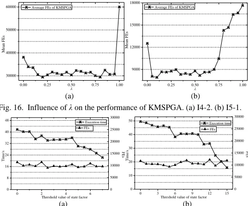
F. Parameter Investigation
We investigate the penalty coefficient λ and the threshold value of state factor ζc in this subsection in order to show how