Improving an Active Shape Model with Random Classification Forest for Segmentation of Cervical Vertebrae

City, University of London Institutional Repository

Citation

:

Al-Arif, S. M., Gundry, M., Knapp, K. and Slabaugh, G. G. (2017). Improving an

Active Shape Model with Random Classification Forest for Segmentation of Cervical

Vertebrae. In: Yao, J., Vrtovec, T., Zheng, G., Frangi, A., Glocker, B. and Li, S. (Eds.),

Improving an Active Shape Model with Random Classification Forest for Segmentation of

Cervical Vertebrae. Lecture Notes in Computer Science, 10182. (pp. 3-15). Cham: Springer.

ISBN 978-3-319-55049-7

This is the accepted version of the paper.

This version of the publication may differ from the final published

version.

Permanent repository link:

http://openaccess.city.ac.uk/15481/

Link to published version

:

Copyright and reuse:

City Research Online aims to make research

outputs of City, University of London available to a wider audience.

Copyright and Moral Rights remain with the author(s) and/or copyright

holders. URLs from City Research Online may be freely distributed and

linked to.

Classification Forest for Segmentation of

Cervical Vertebrae

S M Masudur Rahman Al Arif1, Michael Gundry2, Karen Knapp2 and Greg

Slabaugh1

1

Department of Computer Science, City University London, UK

2_{University of Exeter Medical School, UK}

Abstract. X-ray is a common modality for diagnosing cervical verte-brae injuries. Many injuries are missed by emergency physicians which later causes life threatening complications. Computer aided analysis of X-ray images has the potential to detect missed injuries. Segmentation of the vertebrae is a crucial step towards automatic injury detection sys-tem. Active shape model (ASM) is one of the most successful and popular method for vertebrae segmentation. In this work, we propose a new ASM search method based on random classification forest and a kernel den-sity estimation-based prediction technique. The proposed method have been tested on a dataset of 90 emergency room X-ray images contain-ing 450 vertebrae and outperformed the classical Mahalanobis distance-based ASM search and also the regression forest-distance-based method.

Keywords: ASM, Classification forest, Cervical, Vertebrae, X-ray.

1

Introduction

The cervical spine or the neck region is vulnerable to high-impact accidents like road collisions, sports mishaps and falls. Cervical radiographs is usually the first choice for emergency physicians to diagnose cervical spine injuries due to the required scanning time, cost, and the position of the spine in the human body. However, about 20% of cervical vertebrae related injuries remain undetected by emergency physicians and roughly 67% of these missing injuries result in tragic consequences, neurological deteriorations and even death [1, 2]. Computer aided diagnosis of cervical X-ray images has a great potential to help the emergency physicians to detect miss-able injuries and thus reducing the risk of missing injury related consequences.

search has been introduced for this task. However, this method is limited to edge like object boundaries. An improved Mahalanobis distance-based search method has been introduced in [13]. This method involves a training phase and an optimization step to find the amount of displacement needed to converge the mean shape on the actual object boundary. The method has been shown to work well on cervical vertebra X-ray images in [3, 4]. In [15], a conventional binary classifier and a boosted regression predictor has been compared and used to improve the performance of ASM segmentation during image search phase. While these methods detect the displacement of the shape towards the possi-ble local minima, [16] have proposed a method to directly predict some of the shape parameters using a classification method. In the state-of-the-art work on vertebra segmentation [17], a random regression forest has used to predict the displacement during image search of constrained local model (CLM), another version of SSM.

In this paper, we propose a one-shot random classification forest-based dis-placement predictor for ASM segmentation of cervical vertebrae. Unlike the Ma-halanobis distance-based method used in [3, 4, 13, 14], this method predicts the displacement directly without a need of a sliding window-based search technique. Our method uses a multi-class forest in contrast with the binary classification method used in [15]. A kernel density estimation (KDE)-based classification label prediction method has been introduced which performed better than traditional classification label prediction method. The proposed algorithm has been tested on a dataset of 90 emergency room X-ray images and achieved 16.2% lower error than the Mahalanobis distance-based method and 3.3% lower fit-failure compared with a regression-based framework.

2

Methodology

Active shape model (ASM) has been used in many vertebrae segmentation frame-works. In this work, we have proposed an improvement in the image search phase of ASM segmentation using a one-shot multi-class random classification forest al-gorithm. The proposed method is compared with a Mahalanobis distance-based method and a random regression forest-based method. The ASM is briefly de-scribed in Sec. 2.1, followed by the Mahalanobis distance-based search method in Sec. 2.3, regression forest-based search method in Sec. 2.4 and finally the proposed search method is explained in Sec. 2.5.

2.1 Active Shape Model

Letxi, a vector of length 2ndescribingn2D points of thei-th registered training

vertebra, is given by:

xi= [xi1, yi1, xi2, yi2, xi3, yi3, ..., xin, yin] (1)

where (xij, yij) is the Cartesian coordinate of thej-th point of thei-th training

vertebra. A mean shape, ¯x, can be calculated by averaging all the shapes:

¯

x= 1

N

N

X

i=1

where N is the number of vertebrae available in the training set. Now, the

covariance, Λ, is given by

Λ= 1

N−1

N

X

i=1

(xi−x¯)(xi−x¯)T (3)

Principal component analysis (PCA) is performed by calculating 2neigenvectors

p_k (k = 1,2, ...,2n) of Λ. The eigenvectors with smaller eigenvalues (λk) are

often result from noise and/or high frequency variation. Thus any shape,xi, can

be approximated fairly accurately only by considering firstmeigenvectors with

largest eigenvalues.

ˆ

xi≈x¯+Psbi; Ps= [p1,p2, ...,pm] (4)

where bi is a set of weights known as shape parameters. The standard practice

to select m is to find the first few eigenvalues, λk’s, that represent a certain

percentage of the total variance of the training data. For any known shape,xi,

shape parameterbi can be computed as:

bi =PTs(xi−x¯) (5)

2.2 ASM Search

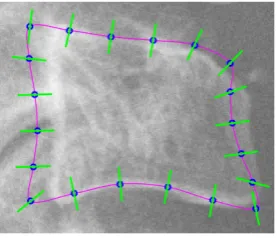
When segmenting a vertebra in a new image, the mean shape is approximately initialized near the vertebra using manually clicked vertebra centers [18,19]. The model then looks for displacement of the mean shape towards the actual vertebra based on the extracted profiles perpendicular to the mean shape in the image (see Fig. 1). In [12], a simple gradient maxima search have been introduced for this task but however this method is limited to edge like object boundaries. An improved Mahalanobis distance-based search method has been introduced in [13]. This method has been used for vertebrae segmentation in [3, 4].

2.3 Mahalanobis distance-based ASM search (ASM-M)

The Mahalanobis distance-based ASM search involves a training phase and an optimization step to find the amount of displacement needed to converge the mean shape on actual object boundary. During training for each landmark point,

intensity profiles of length 2l+1 are collected from all the objects. The normalized

first derivatives these profiles (g) are then used to create a mean profile (¯g) and a

covariance matrix (Λg). When a new profile,gk, is given, then the Mahalanobis

distance can be calculated as:

M(gk) = (gk−¯g)Λ−

1

g (gk−¯g) (6)

The profile gk is then shifted from the mean shape inwards and outwards by

l pixels and Mahalanobis distance is computed at each position. The desired

amount of displacement ˆ(k) is then computed by minimizing M(g_k), which is

equivalent to maximizing the probability thatg_k originates from a

multidimen-sional Gaussian distribution learned from the training data. The one-dimenmultidimen-sional

displacements ˆ(k) for all the points are then mapped into 2D displacement vector

dx. Thisdxreconfigures the mean shape towards the actual object boundary.

db=PTsdx; bt=bt−1+db; xˆt= ˆxt−1+Psbt (7)

where ˆx0= ¯xandb0 is an all zero vector. The process is iterative. The

recon-figuration stops if number of iterations,t, crosses a maximum threshold ordxis

negligible.

2.4 Random Regression Forest-based ASM search (ASM-RRF)

Regression-based method has been used for ASM search in [15]. Random for-est (RF) is a powerful machine learning algorithm [20]. It can be applied to achieve classification and/or regression [21]. Recent state-of-the-art work on ver-tebrae segmentation [17], proposed a random forest regression voting (RFRV) method for this purpose in the CLM framework. The regressor predicts a 2D displacement for the shape to move towards a local minimum. In order to com-pare the performance of our proposed one-shot multi-class random classification forest-based ASM search, a random regression forest-based ASM search has also been implemented. This forest trains on the gradient profiles collected during a training phase and predicts a 1D displacement during ASM search.

ASM-RRF Training: The ASM-M produces a displacement ˆkby minimizing

Eqn. 6 over a range of displacements. The predicted displacement ˆ(k) can take

any value from−lto +lrepresenting the amount of shift needed. The ASM-RRF

is also designed to produce the same, only by looking at the gradient profile (g).

To achieve this, the profile vectors (g) for each landmark point are collected

segmentation pixel with respect to the center. To make the process equivalent to

the previous ASM-M method, the amount of shifting was limited to ±l pixels,

giving us a total of 2l+ 1 regression target values to train the forest. The forest

is trained using standard information gain and regression entropy i.e. variance of the target values.

IG=H(S)− X

i{L,R}

|Sl_|

S H(S

i_{) (8)}

H(S) =Hreg(S) =V ar(LS) (9)

where S is a set of examples arriving at a node and SL_,SR _{are the data that}

travel left or right respectively and LS is the set of target value available at

the node considered. In our case, LS ⊂ {−l,−l+ 1, ...,0, ..., l−1, l}. The node

splitting stops when the tree reaches a maximum depth (Dmax) or number of

elements at node falls below a threshold (nM in). The leaf node records the

statistics of the node elements by saving the mean displacement, ¯kln and the

standard deviationσkln of the node target values.

ASM-RRF Prediction: At test time new profiles are fed into the forest and they regress down to the leaf nodes of different trees. A number of voting

strategies for regression framework are compared in [17]: a single vote at ¯kln, a

probabilistic voting weighted byσkln or a Gaussian spread of votesN(¯kln, σkln).

They reported the best performance using the single vote method. Following

this, in this paper, the displacement ˆkis determined by Eqn. 10. This ˆkis then

returned to the ASM search process to reconfigure the shape for next iteration.

ˆ

k= 1

T

T

X

t=1

(¯klnt) (10)

whereT is the number of trees in the forest.

2.5 Random Classification Forest-based ASM search (ASM-RCF)

The main contribution of this work is to provide an alternative to the already proposed ASM-M and ASM-RRF methods with the help of random classification forest (ASM-RCF) algorithm. Classification-based ASM search methods have previously been investigated in [15, 16]. A binary classification-based method is proposed in [15] to predict the displacement while [16] proposed another classification-based to determine first few shape parameters directly. Like [15] our also ASM-RCF method determines the displacement but instead of a binary classification, the problem is designed as a multi-class classification problem. Thus like regression, it can predict the displacement in one-shot without the need of sliding window search like ASM-M method and [15].

ASM-RCF Training: The training data is the same as the ASM-RRF method.

Gradient profiles (g) are collected using manual segmentations and shifted

the shift labels as continuous regression target values, here we consider them as discrete classification labels. The classification forest is then trained to predict

2l+ 1 class labels. The same information gain of Eqn. 8 is used but the entropy

H(S) is replaced by the classification entropy of Eqn. 11.

H(S) =Hclass(S) =−

X

cC

p(c)log(p(c)) (11)

where C is the set of classes available at the node considered. Here, C ⊂

{−l,−l+1, ...,0, ..., l−1, l}. Both ASM-RRF and ASM-RCF are parametrized by

maximum depth (Dmax), minimum node element (nM in), number of trees (T),

numbers of random variables (nV ar) and numbers of random threshold values

(nT hresh) to considers for node optimization.

ASM-RCF Prediction: The leaf nodes of our classification forest are

associ-ated with a set of labels,Clnxy, that contains all the target classification labels

present at that leaf node.

Clnxy ={c1, c2, ...., cnLeafxy} (12)

wherenLeafxy is the number of elements at thex-th leaf node ofy-th tree of the

forest. At test time, a new profile is fed into the forest and it reaches different leaf nodes of different trees. We have experimented with two different prediction

methods. First, a classical ArgM ax based classification label predictors and

other is a Gaussian kernel-based classification label predictor.

ArgMax based label prediction (RCF-AM):The set of leaf node labels

from each tree is collected inCf orest. The collection of labels is then converted

into a probabilistic distribution over the 2l+ 1 classification labels asp(Cf orest).

Finally, the predicted label ˆc (or the displacement ˆk) is determined by finding

the label that maximizesp(Cf orest).

ˆ

k= ˆcargmax= arg max

c p(Cf orest) (13)

where _{Cf orest={Ctree}

1∪Ctree2∪....∪CtreeT} (14)

Ctreey =Clnxy ={c1, c2, ...., cnLeafxy} (15)

Kernel based label prediction (RCF-KDE): Apart from the RCF-AM method, we propose a new kernel density estimator (KDE) based method to

determine the classification label ˆc or the displacement ˆk of the test profile.

KDE-based predictors are most commonly used in regression forests. But here, we demonstrate its usefulness as a multi-class label predictor for classification

forest. Like RCF-AM, here we also collect the all the leaf node labels asCf orest.

Then at each element cin of Cf orest a zero mean Gaussian distribution with

variance σ2_kde is added. The predicted class ˆc is determined by the label that

maximizes the resultant distribution.

ˆ

k= ˆc= arg max

c

1

s

s

X

i=1

1

σkde √

2πexp

−(x−cini)2

2σ2

kde

!

(16)

where s is number of class labels in Cf orest. Fig. 2 shows an toy example of

-7 -6 -5 -4 -3 -2 -1 0 1 2 3 4 5 6 7 Target shift labels in a leaf node

0 2 4 6 8 10 12 14

Number of samples per label

Fig. 2.An example leaf node and different prediction methods: In this particular leaf node there are in total 40 samples: the shift labels are -5, -4, -3, -2 and 4; number of samples per label are 6, 10, 7, 5 and 12 respectively. The regression mean of ASM-RRF method for this leaf node is zero, class label prediction with ArgMax (ASM-RCF-AM) method is label 5 and with ASM-RCF-KDE method is label -4. The magenta curve represents the summed kernel densities.

3

Experiments

3.1 Data

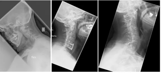
A total of 90 X-ray images have been used for this work. Different (Philips, Agfa, Kodak, GE) radiographic systems were used for the scans. Pixel spacing varied from 0.1 to 0.194 pixel per millimetre. The dataset is very challenging and contains natural variations, deformations, injuries and implants. A few images from the dataset are shown in Fig. 3. Each of these images was then manually

Fig. 3.Example of images in the dataset.

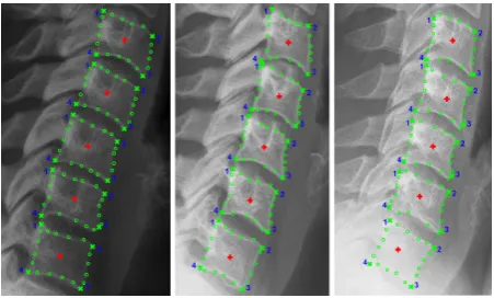
studied in this work due to their ambiguity in lateral X-ray images similar to other work in the literature [3, 4].

Fig. 4.Manual segmentations: centers (+), corners (×) and other points (o).

3.2 Training

An ASM is trained for each vertebra separately. Five models are created for five vertebrae. The means and covariance matrices for ASM-M are computed separately for each landmark point of each vertebra. The forests (ASM-RRF and ASM-RCF) are trained separately for each side of the vertebrae (anterior, posterior, superior and inferior). To increase the forest training samples, the 20 point segmentation shape is converted into a 200 point shape using Catmull-Rom spline. The training profiles are collected from these points. The training

profiles for all ASM search methods are of length 27 i.e.l= 13, giving us a total

of 27 shift labels:{−13,−12, ...,0, ...,12,13}.

3.3 Segmentation evaluation

A 10-fold cross-validation scheme has been followed. For each fold, the ASM, ASM-M, ASM-RRF and ASM-RCF training has been done on 81 images and tested on 9 images. After training, each fold consists of 5 vertebrae ASM models

(mean shape, Eigen vectors and Eigen values), (5 vertebra ×20 points =) 100

mean gradient profiles and covariance matrices for ASM-M method and (5 ×4

sides =) 20 forests each for ASM-RRF and ASM-RCF methods. Each forest is

trained on (200 points ×27 labels × 81 training images ÷4 sides =) 109350

3.4 Parameter optimization

There are five free parameters in the random forest training: the number of trees

(T), maximum allowed depth of a tree (Dmax), minimum number of elements

at a node (nM in), number of variables to look at in each split nodes (nV ar)

and number of thresholds (nT resh) to consider per variable. Apart from these,

the kernel density estimation function requires a bandwidth (BW) which is the

varianceσ2

kde of Eqn. 16. A greedy sequential approach is employed to optimize

each parameter due to time constraint. The sequence followed is: BW, T, D

and nM in in a 2D fashion, and nV arand nT hreshin a 2D fashion. The cost function for the optimization is the average absolute difference between predicted

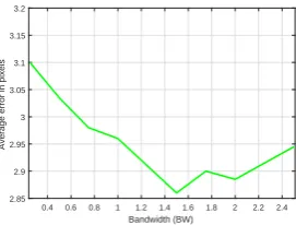
and actual class labels. Fig. 5 shows an example parameter search forBW.BW

is chosen based on the minimum error found on the graph i.e. 1.5. Similarly, all the parameters are optimized and reported in Table 1.

0.4 0.6 0.8 1 1.2 1.4 1.6 1.8 2 2.2 2.4

Bandwidth (BW)

2.85 2.9 2.95 3 3.05 3.1 3.15 3.2

Average error in pixels

Fig. 5.Bandwidth Optimization.

Table 1.Optimized parameters.

Parameters Value

BW 1.5

T 100

Dmax 10

nM in 50

nV ar 6

nT hresh 5

4

Results

of the vertebrae. The performance is satisfactory for the vertebrae with low con-trast (4a) and implants (5a) too. But the algorithm still requires future work. Row (b) of Fig. 7 shows challenging segmentation cases where the segmentation was unsuccessful. It can be seen that the segmentation sometimes suffers from low contrast and bad initialization (1b), deformity (2b) and implants (3b,4b and 5b).

Table 2.Performance comparison: average error in MM.

ASM-M ASM-RRF ASM-RCF-AM ASM-RCF-KDE

Median 0.8019 0.6933 0.7054 0.6896

Mean 0.8582 0.7704 0.8060 0.7688

Standard deviation 0.3437 0.3766 0.3998 0.3965

Fit failures (%Errors>1 mm) 24.00 21.78 20.00 16.67

0 0.5 1 1.5 2 2.5 3 3.5

Mean point-to-curve error (mm)

0 0.1 0.2 0.3 0.4 0.5 0.6 0.7 0.8 0.9 1

Proportion of vertebrae

Performance Curve

ASM-RCF-KDE ASM-RRF ASM-RCF-AM ASM-M

0.5 1 1.5

Mean point-to-curve error (mm)

0 0.1 0.2 0.3 0.4 0.5 0.6 0.7 0.8 0.9

Proportion of vertebrae

Performance Curve

ASM-RCF-KDE ASM-RRF ASM-RCF-AM ASM-M

Fig. 6.Comparison of performance.

Fig. 7.Segmentation results: Manual segmentation (green), ASM-RCF-KDE (blue).

5

Conclusion

search process. The new algorithm has been formulated as a classification prob-lem which eliminates the sliding window search of Mahalanobis distances-based method. The improved algorithm provides better segmentation results and an improvement of 16.1% in point to line segmentation errors has been achieved for a challenging dataset over ASM-M. The proposed classification forest-based framework with kernel density-based prediction (ASM-RCF-KDE) outperformed regression-based methods by 3.3% in terms of fit-failures. The proposed KDE-based prediction helps to predict the displacement with better accuracy because it can nullify the effect of false tree predictions by using information from neigh-bouring classes (Fig 2).

Our algorithm has been tested on a challenging dataset of 90 emergency room X-ray images containing 450 cervical vertebrae. We have achieved a lowest aver-age error of 0.7688 mm. In comparison, current state-of-the-art work [17], reports an average error of 0.59 mm for a different dataset of DXA images on healthy thoraco-lumbar spine. Their method uses the latest version of SSM, constrained local model (CLM) with random forest regression voting based search method. In the near future, we plan to work on CLM with a classification forest-based search method. As our overarching goal is to develop an injury detection sys-tem, the segmentation still requires further work to apply morphometric analysis to detect injuries especially for the vertebrae with conditions like osteoporosis, fractures and implants. Our work is currently focused on improving the segmen-tation accuracy by experimenting with better and automatic initialization using vertebrae corners [18, 19] and/or endplates [5].

References

1. P. Platzer, N. Hauswirth, M. Jaindl, S. Chatwani, V. Vecsei, and C. Gaebler, “Delayed or missed diagnosis of cervical spine injuries,” Journal of Trauma and Acute Care Surgery, vol. 61, no. 1, pp. 150–155, 2006.

2. J. W. Davis, D. L. Phreaner, D. B. Hoyt, and R. C. Mackersie, “The etiology of missed cervical spine injuries.,” Journal of Trauma and Acute Care Surgery, vol. 34, no. 3, pp. 342–346, 1993.

3. M. Benjelloun, S. Mahmoudi, and F. Lecron, “A framework of vertebra segmenta-tion using the active shape model-based approach,”Journal of Biomedical Imaging, vol. 2011, p. 9, 2011.

4. S. A. Mahmoudi, F. Lecron, P. Manneback, M. Benjelloun, and S. Mahmoudi, “GPU-based segmentation of cervical vertebra in X-ray images,” inCluster Com-puting Workshops and Posters (CLUSTER WORKSHOPS), 2010 IEEE Interna-tional Conference on, pp. 1–8, IEEE, 2010.

5. M. G. Roberts, T. F. Cootes, and J. E. Adams, “Automatic location of vertebrae on DXA images using random forest regression,” inMedical Image Computing and Computer-Assisted Intervention–MICCAI 2012, pp. 361–368, Springer, 2012. 6. M. G. Roberts, T. F. Cootes, and J. E. Adams, “Vertebral shape: automatic

mea-surement with dynamically sequenced active appearance models,” inMedical Im-age Computing and Computer-Assisted Intervention–MICCAI 2005, pp. 733–740, Springer, 2005.

inMedical Image Computing and Computer-Assisted Intervention–MICCAI 2009, pp. 1017–1024, Springer, 2009.

8. M. Roberts, E. Pacheco, R. Mohankumar, T. Cootes, and J. Adams, “Detection of vertebral fractures in DXA VFA images using statistical models of appearance and a semi-automatic segmentation,” Osteoporosis international, vol. 21, no. 12, pp. 2037–2046, 2010.

9. S. Casciaro and L. Massoptier, “Automatic vertebral morphometry assessment,” inEngineering in Medicine and Biology Society, 2007. EMBS 2007. 29th Annual International Conference of the IEEE, pp. 5571–5574, IEEE, 2007.

10. M. A. Larhmam, S. Mahmoudi, and M. Benjelloun, “Semi-automatic detection of cervical vertebrae in X-ray images using generalized hough transform,” in Image Processing Theory, Tools and Applications (IPTA), 2012 3rd International Con-ference on, pp. 396–401, IEEE, 2012.

11. M. A. Larhmam, M. Benjelloun, and S. Mahmoudi, “Vertebra identification using template matching modelmp and K-means clustering,” International journal of computer assisted radiology and surgery, vol. 9, no. 2, pp. 177–187, 2014.

12. T. F. Cootes, C. J. Taylor, D. H. Cooper, and J. Graham, “Active shape models-their training and application,”Computer vision and image understanding, vol. 61, no. 1, pp. 38–59, 1995.

13. T. Cootes and C. Taylor, “Statistical models of appearance for computer vision, wolfson image anal. unit, univ. manchester, manchester,” tech. rep., UK, Tech. Rep, 1999.

14. B. Van Ginneken, A. F. Frangi, J. J. Staal, B. M. Romeny, and M. A. Viergever, “Active shape model segmentation with optimal features,”medical Imaging, IEEE Transactions on, vol. 21, no. 8, pp. 924–933, 2002.

15. D. Cristinacce and T. F. Cootes, “Boosted regression active shape models.,” in

BMVC, vol. 1, p. 7, 2007.

16. Y. Zheng, A. Barbu, B. Georgescu, M. Scheuering, and D. Comaniciu, “Four-chamber heart modeling and automatic segmentation for 3-D cardiac CT volumes using marginal space learning and steerable features,”IEEE transactions on med-ical imaging, vol. 27, no. 11, pp. 1668–1681, 2008.

17. P. Bromiley, J. Adams, and T. Cootes, “Localisation of vertebrae on DXA images using constrained local models with random forest regression voting,” in Recent Advances in Computational Methods and Clinical Applications for Spine Imaging, pp. 159–171, Springer, 2015.

18. S. M. M. R. Al-Arif, M. Asad, K. Knapp, M. Gundry, and G. Slabaugh, “Hough forest-based corner detection for cervical spine radiographs,” inMedical Image Un-derstanding and Analysis (MIUA), Proceedings of the 19th Conference on, pp. 183– 188, 2015.

19. S. M. M. R. Al-Arif, M. Asad, K. Knapp, M. Gundry, and G. Slabaugh, “Cervical vertebral corner detection using Haar-like features and modified Hough forest,” in

Image Processing Theory, Tools and Applications (IPTA), 2015 5th International Conference on, IEEE, 2015.

20. L. Breiman, “Random forests,”Machine learning, vol. 45, no. 1, pp. 5–32, 2001. 21. J. Gall, A. Yao, N. Razavi, L. Van Gool, and V. Lempitsky, “Hough forests for