FAemb: a function approximation-based embedding method for image retrieval
Thanh-Toan Do
Quang D. Tran
Ngai-Man Cheung
Singapore University of Technology and Design
{thanhtoan do, quang tran, ngaiman cheung}@sutd.edu.sgAbstract
The objective of this paper is to design an embed-ding method mapping local features describing image (e.g. SIFT) to a higher dimensional representation used for im-age retrieval problem.
By investigating the relationship between the linear ap-proximation of a nonlinear function in high dimensional space and state-of-the-art feature representation used in im-age retrieval, i.e., VLAD, we first introduce a new approach for the approximation. The embedded vectors resulted by the function approximation process are then aggregated to form a single representation used in the image retrieval framework.
The evaluation shows that our embedding method gives a performance boost over the state of the art in image re-trieval, as demonstrated by our experiments on the standard public image retrieval benchmarks.
1. Introduction
The problem of finding a single vector representing a set of local vectors describing an image is an important prob-lem in computer vision. This is because the single rep-resentation provides two main benefits. First, it contains the power of local descriptors, such as set of SIFT de-scriptors [17]. Second, the single represented vectors can be either compared with standard distances used in image retrieval problem or used by robust classification methods such as SVM in classification problem.
There is a wide range of methods for finding a sin-gle vector to represent a set of local vectors proposed in the literature such as bag-of-visual-words (BoW) [28], Fisher vector [22], vector of locally aggregated descriptor (VLAD) [12] and its improvements [7,2], super vector cod-ing [33], vector of locally aggregated tensor (VLAT) [26,
20] which is higher order (tensor) version of VLAD, trian-gulation embedding (Temb) [14], sparse coding [21], local coordinate coding (LCC) [32], locality-constrained linear coding [29] which is fast version of LCC, local coordinate coding using local tangent (TLCC) [31] which is higher
or-der version of LCC. Among these methods, VLAD [13] and VLAT [20] are well-known embedding methods used in im-age retrieval problem [13,20] while TLCC [31] is one of successful embedding methods used in image classification problem.
VLAD is designed for image retrieval problem while TLCC is designed for image classification problem. They also come from different motivations. VLAD’s motivation is to characterize the distribution of residual vectors over Voronoi cells learned by a quantizer while TLCC’s motiva-tion is tolinearly approximate1a nonlinear function in high dimensional space. Despite above differences, we show that VLAD is actually simplified version of TLCC. This means that we can depart from the idea of linear approximation of function to develop good embedding methods for image retrieval problem.
To find the single representation, all aforementioned methods include two main steps in the processing: embed-ding and aggregating. The embedembed-ding step maps each local descriptor to a high dimensional vector while the aggregat-ing step converts set of mapped high dimensional vectors to a single vector. This paper focuses on the first step. In particular, we develop a new embedding method which can be seen as the generalization of TLCC and VLAT.
In next sections, we first present a brief description of TLCC and show the relationship between TLCC and VLAD. We then present our motivation for designing new embedding method.
1.1. TLCC
TLCC [31] is designed for image classification problem. Its goal is to linearly approximate a smooth nonlinear func-tion f(x),i.e. a nonlinear classification function, defined on a high dimensional feature spaceRd. TLCC’s approach finds an embedding scheme φ: Rd → RD mapping each
x∈Rdas
x→φ(x) (1)
1The meaning of “linear approximation” in this paper is that the
non-linear functionf(x)defined onRdis approximated by a linear function
such thatf(x)can be well approximated by a linear func-tion, namelywTφ(x). To solve above problem, TLCC’s au-thors relied on the idea of coordinate coding defined bellow. They showed that with a sufficient selection of coordinate coding, the functionf(x)can be linearly approximated.
Definition 1.1 Coordinate Coding [32]
A coordinate coding of a pointx∈Rdis a pair(γ(x),C)2, where C = [v1, . . . ,vn] ∈ Rd×n is a set of n anchor
points (bases), and γ is a map of x ∈ Rd to γ(x) =
[γv
1(x), . . . , γvn(x)]
T ∈
Rnsuch that
n
j=1
γvj(x) = 1 (2)
It induces the following physical approximation ofxinRd:
x′ =
n
j=1
γvj(x)vj (3)
A good coordinate coding should ensure that x′ closes to x3.
Let(γ(x),C)be coordinate coding ofx. Under assump-tion thatf is(α, β, ν)Lipschitz smooth, they showed (in lemma 2.2 [31]) that, for allx∈Rd
f(x)−
n
j=1 γvj(x)
f(vj) +1
2∇f(vj)
T(x−v j)
≤ 1
2αx−x
′ 2+ν
n
j=1
|γvj(x)| x−vj
3
2 (4)
To ensure a good approximation of f(x), they mini-mize the RHS of (4). (4) further means that the func-tionf(x)can be linearly approximated bywTφ(x)where
w =1 sf(vj);
1
2∇f(vj)
n
j=1 and TLCC embeddingφ(x) defined as
φ(x) =
sγvj(x);γvj(x)(x−vj)
n j=1∈R
n(1+d) (5)
wheresis a nonnegative constant.
1.2. TLCC as generalization of VLAD
Although TLCC is designed for classification problem and its motivation is different from VLAD, TLCC can be seen as a generalization of VLAD.
If we add following constraint toγ(x)
γ(x)
0= 1 (6)
2Cis same for allx.
3Although the reconstruction error condition for a good coordinate
cod-ing, i.e,x′
closes tox, is not explicit mentioned in original definition of coordinate coding, it can be inferred from objective functions of LCC [32] and TLCC [31].
then we havex≈x′ =v∗. The RHS of (4) becomes
1
2αx−v∗2+νx−v∗ 3
2 (7)
wherev∗is anchor point corresponding to nonzero element of γ(x). One of solutions for minimizing (7) under con-straints (2) and (6) is K-means algorithm. When K-means is used, we have
v∗= argmin
v∈C
x−v
2 (8)
where C is set of anchor points learned by K-means. Now, considering (5), if we choose s = 0 and we remove zero elements attached with s, φ(x) =
0, . . . ,0,(x−v∗)T,0, . . . ,0T
∈ Rnd will become VLAD.
1.3. Motivation for designing new embedding
method
The relationship between TLCC and VLAD means that if we can findφ(x)such thatf(x)can be well linearly ap-proximated (f(x) ≈ wTφ(x)), we then can use φ(x)for image retrieval problem. However, in TLCC’s approach, by departing from assumption thatf is(α, β, ν)Lipschitz smooth,fis approximated using only its first order approx-imation at anchor points,i.e.,f is approximated as sum of weighted tangents at anchor points. It is not straightforward to use the TLCC framework to have a better approximation, for examples, approximation off using its second order or higher order approximation at anchor points.
Therefore, in this paper, we propose to use Taylor expan-sion for function approximation and it is more straightfor-ward to achieve a higher order approximation offat anchor points by this way. The embedded vectors, resulted by the function approximation process, will be used as new image representations in our image retrieval framework. In fol-lowing sections, we will note ourFunctionA pproximation-basedembedding method asFAemb.
The remaining of this paper is organized as follows. Sec-tion2introduces related background. Section3introduces FAemb embedding method. Section4presents experimen-tal results. Section5concludes the paper.
2. Preliminaries
In this section, we review related background preparing for detail presenting of new embedding method in section3.
Taylor’s theorem for high dimensional variables
Definition 2.1 Multi-index [8]: A multi-index is ad-tuple of nonnegative integers. Multi-indices are generally de-noted byα:
where(αj ∈ {0,1,2, ...}). Ifαis a multi-index, we define
|α|=α1+α2+· · ·+αd;α! =α1!α2!. . . αd!
xα=x1α1x
2α2. . . xdαd
∂αf(x) = ∂ |α|f(x)
∂α1(x1)∂α2(x2). . . ∂αd(xd)
wherex= (x1, x2, . . . xd)T ∈Rd
Theorem 2.2 (Taylor’s theorem for high dimensional vari-ables) [8]Supposef:Rd→Rof class ofCk+14on
Rd. If a∈Rdanda+h∈Rd, then
f(a+h) = |α|≤k
∂αf(a)
α! h
α+R
a,k(h) (9)
whereRa,k(h)is Lagrange remainder given by
Ra,k(h) =
|α|=k+1
∂αf(a+ch)h
α
α! (10)
for somec∈(0,1).
Corollary 2.3 If f is of class of Ck+1 on Rd and
|∂αf(x)| ≤M forx∈Rdand|α|=k+ 1, then
|Ra,k(h)| ≤ M
(k+ 1)!h
k+1
1 (11)
The proof of corollary2.3is given in [8]
3. Embedding based on function
approxima-tion (FAemb)
In this section, we introduce our embedding method. It is inspired from function approximation based on Taylor’s theorem represented in previous section.
3.1. Derivation of FAemb
Lemma 3.1 Iff: Rd →Ris of class ofCk+1 onRdand
∇kf(x)is Lipschitz continuous with constantM >0and
(γ(x),C)is coordinate coding ofx, then
f(x)−
n
j=1 γvj(x)
|α|≤k
∂αf(v j)
α! (x−vj)
α
≤ M
(k+ 1)!
n
j=1
|γvj(x)| x−vjk1+1 (12)
4It means that all partial derivatives offup to (and including) order
k+ 1exist and continuous.
The proof of Lemma3.1is given in AppendixA.1. Ifk= 1, then (12) becomes
f(x)−
n
j=1 γvj(x)
f(vj) +∇f(vj)T(x−vj)
≤ M
2
n
j=1
|γvj(x)| x−vj
2
1 (13)
In the case of k = 1, f is approximated as sum of its weighted tangents at anchor points.
Ifk= 2, then (12) becomes
f(x)−
n
j=1 γvj(x)
f(vj) +∇f(vj)T(x−vj)
+1 2
V
∇2f(v j)
T
V
(x−vj)(x−vj)T
≤ M
6
n
j=1
|γvj(x)| x−vj3
1 (14)
whereV(A)is vectorization function flattening the matrix Ato a vector by putting its consecutive columns into a col-umn vector.∇2is Hessian matrix.
In the case ofk = 2,f is approximated as sum of its weighted quadratic approximations at anchor points.
To achieve a good approximation, the coding(γ(x),C) should be selected such that the RHS of (13) and (14) are small enough.
The result derived from (13) is that, with respect to the coding (γ(x),C), a high dimensional nonlinear function f(x)inRd can be approximated by linear formwTφ(x) wherewcan be defined asw=1
sf(vj);∇f(vj)
n
j=1and the embedded vectorφ(x)can be defined as
φ(x) =
sγvj(x);γvj(x)(x−vj)
n
j=1∈R n(1+d)
(15)
wheresis a nonnegative scaling factor to balance two types of codes.
To make a good approximation of f, in following sections, we put our interest on case where f is ap-proximated by using up to second-order derivatives de-fined by (14). The result derived from (14) is that the nonlinear function f(x) can be approximated by lin-ear form wTφ(x) where w can be defined as w =
1 s1f(
vj); 1
s2∇f(
vj);1 2
V
∇2f(v j)
n
j=1 and the em-bedded vectorφ(x)-FAemb can be defined as
φ(x) =
s1γvj(x);s2γvj(x)(x−vj);
γvj(x)V
(x−vj)(x−vj)T n
j=1∈R
n(1+d+d2)
(16)
3.2. Learning of coordinate coding
As mentioned in previous section, to get a good ap-proximation of f, the RHS of (14) should be small enough5. Furthermore, from definition of coordinate cod-ing1.1,(γ(x),C)should ensure that the reconstruction er-rorx′−x
2should be small. Putting two above criteria together, we find(γ(x),C)which minimize the following constrained objective function
Q(γ(x),C) =x−Cγ(x)2 2+μ
n
j=1
|γvj(x)| x−vj31
st.1Tγ(x) = 1 (17)
Equivalently, given a set of training samples (descriptors) X = [x1, . . . ,xm] ∈ Rd×m, let γ
ij be coefficient
corre-sponding to basevj of samplexi;γi = [γi
1, . . . , γin]
T ∈
Rnbe coefficient vector of samplex
i;Γ = [γ1, . . . , γm]∈
Rn×m. We find(Γ,C)which minimize the following con-strained objective function
Q(Γ,C) =
m
i=1
⎡
⎣xi−Cγi22+μ n
j=1
|γij| xi−vj 3 1
⎤
⎦
st.1Tγi = 1, i= 1, . . . , m (18)
To minimize (18), we iteratively optimize it by alternatingly optimizing with respect toCandΓwhile holding the other fixed.
For learning the coefficientsΓ, the optimization problem is equivalent to a regularized least squares problem with lin-ear constraint. This problem can be solved by optimizing over each samplexiindividually. To findγiof each sample xi, we use Newton’s method [4]. The gradient and Hessian of objective function w.r.t.γiis given in AppendixA.2.
For learning the bases C, the optimization problem is unconstrained regularized least squares. We use trust-region method [6,5] to solve this problem6. The gradient and Hes-sian of objective function w.r.t.Cis given in AppendixA.2. After learningC, given a new descriptorx, we getγ(x) by minimizing (17) using learnedC. Fromγ(x), we get the embedded vectorφ(x)-FAemb by using (16).
3.3. Relationship to other methods
The most related embedding methods to FAemb are TLCC [31] and VLAT [26].
Compare to TLCC [31], our assumption on f in lemma3.1is slightly different from assumption of TLCC (lemma2.2[31]). Our assumption only needs that∇kf(x)
5BecauseM
6 is constant, it can be ignored in the optimization process.
6Because the objective function involvesL
1norm, some methods de-signed forL1regularization, i.e, feature-sign search algorithm [16], can be used. However, we find that the Newton’s method (for computingΓ) and the trust-region method (for computingC) work well in practice.
is Lipschitz continuous while TLCC assumes that all
∇jf(x)are Lipschitz continuous,j= 1, . . . , k. Our objec-tive function (17) is also different from TLCC (4). We rely onL1norm of (x−vj) in the second term while TLCC uses
L2 norm. We solve the constraint on the coefficientγ in our optimization process while TLCC does not. FAemb ap-proximatesf using up to its second order derivatives while TLCC approximatesf only using its first order derivatives. FAemb can also be seen as the generalization of VLAT [26]. Similar to the relationship of TLCC and VLAD presented in section 1.2, if we add constraint (6) toγ(x) then the objective function (18) will become
Q1(Γ,C) = m
i=1
xi−v∗2
2+μxi−v∗31
st.1Tγi = 1, i= 1, . . . , m
γi0= 1, i= 1, . . . , m (19)
wherev∗is anchor point corresponding to nonzero element ofγi.
If we relaxL1norm in the second term ofQ1(Γ,C)into L2norm, then we can use K-means algorithm for minimiz-ing (19). After learningCby using K-means, given an input descriptorx, we have
x≈v∗= argmin
v∈C
x−v
2 (20)
Now, consider (16), if we choose s1 = 0, s2 = 0 and we remove zero elements attached with them, φ(x) =
[0, . . . ,0,
V
(x−v∗)(x−v∗)T T
,0, . . . ,0]T ∈ Rnd2
will become VLAT.
In practice, to make a fair comparison between FAemb and VLAT, the embedded vectors producing by two meth-ods should have same dimension. To ensure this, we choose
s1, s2in (16) equal to0. It is worth noting that in (16), as matrix(x−vj)(x−vj)T is symmetric, only the diagonal and upper part are kept while flattening it into vector. The size of VLAT and FAemb is then nd(d2+1).
3.4. Whitening and aggregating embedded vectors
to single vector
3.4.1 Whitening
In [14], authors showed that by applying the whitening pro-cessing, the discriminating of embedded vectors can be im-proved, hence improving the retrieval results.
In particular, given φ(x) ∈ RD, we achieve whitened embedded vectorsφw(x)by
φw(x) =diag
λ−12
1 , . . . , λ −1
2
D
PTφ(x) (21)
largest eigenvalues of the covariance matrix computed from learning embedded vectorsφ(x).
[14] further suggested that by discarding some first com-ponents associated with the largest eigenvalues of φw(x), the localization of whitened embedded vectors will be im-proved. In practice, we also apply this truncation operation. The detail of this truncation operation is presented in sec-tion4.
3.4.2 Aggregating
Let X = {x} be set of local descriptors describing the image. Sum-pooling [15] and max-pooling [30, 3] are two common methods for aggregating set of whitened embedded vectors φw(x) of the image to a single vec-tor. Sum-pooling lacks discriminability because the ag-gregated vector is more influenced by frequently-occurring uninformative descriptors than rarely-occurring informa-tive ones. Max-pooling equalizes the influence of fre-quent and rare descriptors. However, classical max-pooling approaches can only be applied to BoW or sparse cod-ing features. Recently, [14] introduced a new aggregating method nameddemocratic aggregationapplied to image re-trieval problem. This method bears similarity to general-ized max-pooling [19] applied to image classification prob-lem. Democratic aggregation can be applied to general fea-tures such as VLAD, Temb, Fisher vector. [14] showed that democratic aggregation achieves better performance than sum-pooling. The main idea of democratic aggregation is to find a weight for eachφw(x)such that∀xi∈ X
λi(φw(xi))T
xj∈X
λjφw(xj) = 1 (22)
Generally, the process to produce the single vector from set of local descriptors describing the image is as follows. First, we map eachx ∈ X → φ(x)and whiteningφ(x), producingφw(x). We then use democratic aggregation to aggregate vectorsφw(x)to the single vectorψby
ψ(X) =
xi∈X
λiφw(xi) (23)
4. Experiments
This section presents results of our FAemb embedding method. In section4.3, we compare FAemb to other three methods: VLAD [13], Temb [14] and VLAT [26]. We reim-plement VLAD and VLAT in our framework. For Temb, we use the source code provided by [14]. To make a fair comparison, the whitening and the aggregating presented in section3.4are applied for all four embedding methods. As suggestion in [14], for Temb and VLAD methods, we dis-carddfirst components ofφw(x). The final dimension of
φw(x)is thereforeD= (n−1)×d. For VLAT and FAemb
methods, we discard d×(d2+1) first components of φw(x). The final dimension ofφw(x)is thereforD=(n−1)d2(d+1). In section 4.4, we compare our framework with image retrieval benchmarks.
The value ofμ in (18) is selected by empirical experi-ments and is fixed to10−3 for all FAemb results reported bellow.
4.1. Dataset and evaluation protocol
INRIA holidays [11] consists of 1491 high resolution im-ages containing personal holiday photos with 500 queries. The search quality is measured by mean average precision (mAP) over 500 queries, with the query removed from the ranked list. As standardly done in the literature, for all the learning stages, we use the independent dataset Flickr60k provided with Holidays.
Oxford buildings (Oxford5k) [24] consists of 5062 im-ages of buildings and 55 query imim-ages corresponding to 11 distinct buildings in Oxford. The search quality is mea-sured by mAP computed over the 55 queries. Images are annotated as either relevant, not relevant, or junk, which indicates that it is unclear whether a user would consider the image as relevant or not. We follow same configuration in [7,14,12] where the junk images are removed from the ranking before computing the mAP. As standardly done in the literature, for all the learning stages, we use the Paris6k dataset [25].
4.2. Implementation notes
Local descriptors are detected using the Hessian-affine detector [18] and described by the SIFT local descrip-tor [17]. We used RootSIFT variant [1] in all our experi-ments.
For VLAT and FAemb, at beginning, all SIFT descriptors are reduced from 128 to 45 dimensions using PCA. This makes the dimension of VLAT and FAemb comparable to dimension of compared embedding methods.
Power-law normalization. The problem of burtiness vi-sual elements is first introduced in [10]: numerous de-scriptors almost similar within the same image. This phe-nomenon strongly affects the measure of similarity between two images. To reduce the effect of burtiness, we simi-larly do as previous works [12, 14]: applying power-law normalization [23] to the final image representationψand subsequently L2 normalize it. The applying of power-law normalization to each component a of ψ is done by
Table 1. The comparison between the implementation of VLAD and VLAT in this paper and their improved versions [13,20] on Holidays dataset.Dis final dimension of aggregated vectors. Ref-erence results are obtained from corresponding papers.
method D mAP
VLAD [13] 16,384 58.7 VLAD (this paper) 8,064 67.4 VLAD (this paper) 16,256 68.3 VLATimproved[20] 9,000 70.0
VLAT (this paper) 7,245 70.9 VLAT (this paper) 15,525 72.7
8 16 32 64 128
55 60 65 70 75 80
number of anchor points (n)
mAP
o
n
H
o
lid
a
ys
VLAD Temb VLAT FAemb
Figure 1. Impact of number of anchor points on the Holidays dataset for different embedding methods: VLAD, Temb, VLAT and our FAemb. Givenn, the dimension of VLAD and Temb is 128×(n−1); the dimension of VLAT and FAemb is 45×46
2 ×
(n−1).
4.3. Impact of parameters and comparison of
meth-ods
It is worth noting that even with a lower dimension, the implementation of VLAD and VLAT in our framework (RootSIFT descriptors, VLAD/VLAT embedding, whiten-ing, democratic aggregation and power-law normalization) achieves better retrieval results than their improved versions reported by the authors [13,20]. The comparison on Holi-days dataset is shown in Table1.
Impact of parameters: the main parameter here is num-ber of anchor pointsn. The analysis for this parameter is shown in Figure1and Figure2for Holidays and Oxford5k datasets, respectively. We can see that the mAP increases with the increasing ofnfor all four methods. For Temb, VLAT and FAemb, the improvement tends to be smaller for largern. For VLAT and FAemb, whenn > 32, the im-provement in mAP is not worth the computation overhead.
Comparison of methods: we find that the following ob-servations are consistent on both Holidays and Oxford5k
8 16 32 64 128
40 45 50 55 60 65 70 75
number of anchor points (n)
mAP
o
n
O
xf
o
rd
5
k
VLAD Temb VLAT FAemb
Figure 2. Impact of number of anchor points on the Oxford5k dataset for different embedding methods: VLAD, Temb, VLAT and our FAemb. Givenn, the dimension of VLAD and Temb is 128×(n−1); the dimension of VLAT and FAemb is 45×46
2 ×
(n−1).
datasets.
• For samen, FAemb and VLAT have same dimension. However, FAemb improves the mAP over VLAT by a fair margin. Whenn= 8, the improvement is+1.8% and+3.9% on Holidays and Oxford5k, respectively. Whenn = 16,32, the improvement is about+3%on both datasets.
• When the dimension is comparable, FAemb signif-icantly improves the mAP over VLAD and Temb. For examples, comparing FAemb at (n = 16, D = 15,525) with VLAD/Temb at (n = 128, D = 16,256), the gain of FAemb over VLAD/Temb is +7.5%/+2% on Holidays and +8.1%/+5% on Ox-ford5k.
4.4. Comparison with the state of the art
In this section, we compare our framework with bench-marks having similar representation, i.e., they represent an image by a single vector. The main differences be-tween compared frameworks are shown in Table 2. Ex-cepting VLATimproved [20], other compared methods and
ours consist of power-law normalization step and use Eu-clidean distance when comparing the aggregated vectors. VLATimproved [20] doesn’t have power-law normalization
and it uses Mahalanobis distance when comparing the ag-gregated vectors. VLADLCS [7] and VLATimproved [20]
don’t have whitening step on final embedded vector (φ(x)) but they first apply PCA on Voronoi cells separately. The sub-embedded vectors on Voronoi cells are then concate-nated to form final embedded vector.
[image:6.612.72.259.113.370.2]Table 2. The difference between compared frameworks. The frameworks are named by embedding methods used. RSIFT means RootSIFT.Do whiteningmeans if whitening is applied on embedded vectors.
Frame Local Do Aggr.
work desc. whitening? method
BoW [13] SIFT No Sum
VLAD [13] SIFT No Sum
Fisher [13] SIFT No Sum
VLADLCS[7] RSIFT No Sum
VLADintra[2] RSIFT No Sum
VLATimproved[20] SIFT No Sum
[image:7.612.59.279.303.460.2]Temb [14] RSIFT Yes Democratic Ours (FAemb) RSIFT Yes Democratic
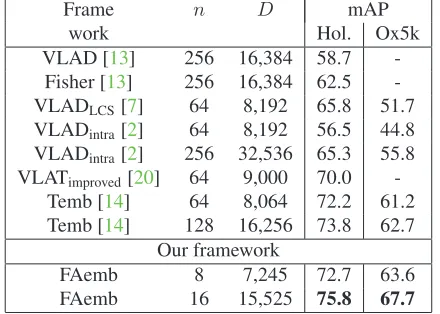
Table 3. Comparison with the state of the art on Holidays and Ox-ford5k datasets. The frameworks are named by embedding meth-ods used.nis number of anchor points.Dis dimension of embed-ded vectors. Reference results are obtained from corresponding papers.
Frame n D mAP
work Hol. Ox5k
VLAD [13] 256 16,384 58.7 -Fisher [13] 256 16,384 62.5 -VLADLCS[7] 64 8,192 65.8 51.7
VLADintra[2] 64 8,192 56.5 44.8
VLADintra[2] 256 32,536 65.3 55.8
VLATimproved[20] 64 9,000 70.0
-Temb [14] 64 8,064 72.2 61.2 Temb [14] 128 16,256 73.8 62.7
Our framework
FAemb 8 7,245 72.7 63.6
FAemb 16 15,525 75.8 67.7
Table3shows that our framework outperforms the com-pared frameworks by a large margin on both datasets. The gain over recent improved VLAD [2] having a high (32,536) dimension is +10.5% on Holidays and +11.9% on Ox-ford5k. Comparing with VLATimproved [20] which is the
latest version of VLAT, the gain is +5.8% on Holidays. Even with a lower dimension, we (D= 7,245) outperform VLATimproved (D = 9,000) +2.7%. Comparing with the
latest embedding method (Temb) [14], we also achieve a gain+2%on Holidays and+5%on Oxford5k.
In Temb embedding [14], to suppress the influence of co-occurrences descriptors that corrupts the similarity mea-sure [9], they applied (before power-law normalization) ro-tation postprocessing introduced in [27] on aggregated vec-tors. For instance, they rotate data with a PCA rotation ma-trix learned on aggregated vectors from learning set. This rotation postprocessing is a complementary operation and it boosts the performance. In this section, we also show results when this operation is applied on our FAemb. To
Table 4. Comparison between Temb [14] and FAemb on Holidays and Oxford5k datasets when rotation postprocessing is applied on the aggregated vector.nis number of anchor points. Dis dimen-sion of embedded vectors. Reference results are obtained from corresponding paper.
n D mAP
Method Hol. Ox5k
Temb + RN [14] 64 8,064 77.1 67.5 Temb + RN [14] 128 16,256 76.8 66.5 FAemb + RN 8 7,245 76.2 66.7 FAemb + RN 16 15,525 78.7 70.9
make a fair comparison with results of Temb [14], we use the same number of learning images as [14]. They are 10k images from Flickr60k for Holidays and 6k images from Paris6k for Oxford5k. The results with the applying of this rotation are noted as +RN, and shown in Table4.
We can see that the applying of the rotation normal-ization to Temb and FAemb gives a large improvement in performance. The mAP of FAemb+RN at D = 7,245
is slightly lower than Temb+RN at D = 8,064 on both datasets. However, we note a larger variance: the best results of FAemb+RN are higher than the best results of Temb+RN, especially on Oxford5k. For instance, the gain is+1.6%on Holidays and+3.4%on Oxford5k.
5. Conclusion
By departing from the goal of linear approximation of a nonlinear function in high dimensional space, this paper proposes a new powerful embedding method for image re-trieval problem. The proposed embedding method-FAemb can be seen as the generalization of several well-known em-bedding methods such as VLAD, TLCC, VLAT. The new presentation compares favorably with state-of-the-art em-bedding methods for image retrieval, such as VLAD, VLAT, Fisher kernel, Temb, even with a shorter presentation.
A. Appendix
A.1. Proof of Lemma
3.1
Because∇kf(x)is Lipschitz continuous with constant
M >0, we have∇k+1f(x)
2≤M. So for|α|=k+ 1,
we have|∂αf(x)| ≤
∇k+1f(x)
We have
f(x)−
n
j=1 γvj(x)
|α|≤k
∂αf(v j)
α! (x−vj)
α = n j=1 γvj(x)
⎛
⎝f(x)−
|α|≤k
∂αf(v j)
α! (x−vj)
α ⎞ ⎠ ≤ n j=1
γvj(x)
⎛
⎝f(x)−
|α|≤k
∂αf(vj)
α! (x−vj)
α ⎞ ⎠ = n j=1 γvj(x)
Rvj,k(x−vj)
≤ M
(k+ 1)!
n
j=1
γvj(x)
x−vjk1+1.
where the last inequation comes from corollary2.3.
A.2. Gradient and Hessian w.r.t.
γi,Cof objective
function
Q(Γ,C)7 We have the objective functionQ(Γ,C) =
m
i=1
⎡
⎣xi−Cγi22+μ n
j=1
|γij| xi−vj 3 1
⎤
⎦
A.2.1 Gradient and Hessian w.r.t.γi
Leta=xi−v13
1,xi−v213, . . . ,xi−vn31
T
, we have
∇Q(γi) = 2CT(Cγi−xi) +μ sign(γi)⊙a(24)
∇2Q(γi) = 2CTC (25)
wheresign(γi) = [sign(γi1), sign(γi2), . . . , sign(γin)]
T
and⊙denotes Hadamard product.
A.2.2 Derivative and Hessian w.r.t.C
LetR=m
i=1xi−Cγi22=X−CΓ 2
2, we have
∇R(C) = 2(CΓ−X)ΓT (26)
Let L = n
j=1
m
i=1|γij| xi−vj 3
1 and let dj =
∇L(vj) = 3m
i=1|γij| vj−xi 2
1sign(vj −xi), we have
∇L(C) = [d1, . . . ,dj, . . . ,dn] (27)
7Theoretically, the partial derivatives∂(Q)/∂γ
ikand∂(Q)/∂vjkdo
not exist at some points. We found, however, the Newton’s method and the trust-region method with the provided derivatives work well in practice.
Finally, we get
∇Q(C) =∇R(C) +μ∇L(C) (28)
Letuj = mi=1γi2j: sum of square of coefficients
cor-responding to base vj of all data points x; let Ajj =
2ujId×d∈Rd×d, j= 1, . . . , n, we have
∇2R(C) =
⎛
⎜ ⎜ ⎜ ⎝
A11 0d×d . . . 0d×d 0d×d A22 . . . 0d×d
..
. ... . .. 0d×d 0d×d 0d×d . . . Ann
⎞ ⎟ ⎟ ⎟ ⎠ (29)
where0d×dis matrix having size ofd×dand zero elements.
LetBjj =∇2L(vj)∈Rd×dbe Hessian ofLw.r.t. base
vj,j= 1, . . . , n, we have
Bjj =
⎛ ⎜ ⎜ ⎜ ⎜ ⎜ ⎝
∂2L
∂vj 1∂vj1
∂2L
∂vj
1∂vj2 . . .
∂2L
∂vj 1∂vjd
∂2L
∂vj 2∂vj1
∂2L
∂vj 2∂vj2
. . . ∂vj∂2L 2∂vjd
..
. ... . .. ... ∂2L
∂vjd∂vj 1
∂2L
∂vjd∂vj 2
. . . ∂2L
∂vjd∂vjd
⎞ ⎟ ⎟ ⎟ ⎟ ⎟ ⎠ (30)
Fork= 1, . . . , d;h= 1, . . . , d; ifk=hthen
∂2L ∂vj
k∂vjh
= 6
m
i=1
|γij| vj−xi1(sign(vjk−xik)) 2
Ifk=hthen
∂2L ∂vj
k∂vjh
= 6
m
i=1
|γij| vj−xi1sign(vjk−xik)sign(vjh−xih)
We have
∇2L(C) =
⎛
⎜ ⎜ ⎜ ⎝
B11 0d×d . . . 0d×d 0d×d B22 . . . 0d×d
..
. ... . .. 0d×d 0d×d 0d×d . . . Bnn
⎞ ⎟ ⎟ ⎟ ⎠ (31)
Finally, we get
∇2Q(C) =∇2R(C) +μ∇2L(C) (32)
References
[1] R. Arandjelovic and A. Zisserman. Three things everyone should know to improve object retrieval. InCVPR, 2012. [2] R. Arandjelovic and A. Zisserman. All about VLAD. In
CVPR, 2013.
[4] S. Boyd and L. Vandenberghe.Convex optimization, p. 528. Cambridge university press, 2004.
[5] T. F. Coleman and Y. Li. On the convergence of interior-reflective newton methods for nonlinear minimization sub-ject to bounds.Mathematical programming, pages 189–224, 1994.
[6] T. F. Coleman and Y. Li. An interior trust region approach for nonlinear minimization subject to bounds.SIAM Journal on optimization, pages 418–445, 1996.
[7] J. Delhumeau, P. H. Gosselin, H. J´egou, and P. P´erez. Revis-iting the VLAD image representation. InMM, 2013. [8] G. B. Folland.Advanced Calculus. Prentice Hall, 1st edition,
2002.
[9] H. J´egou and O. Chum. Negative evidences and co-occurences in image retrieval: The benefit of PCA and whitening. InECCV, 2012.
[10] H. J´egou, M. Douze, and C. Schmid. On the burstiness of visual elements. InCVPR, 2009.
[11] H. J´egou, M. Douze, and C. Schmid. Improving bag-of-features for large scale image search.IJCV, pages 316–336, 2010.
[12] H. J´egou, M. Douze, C. Schmid, and P. P´erez. Aggregating local descriptors into a compact image representation. In
CVPR, 2010.
[13] H. J´egou, F. Perronnin, M. Douze, J. S´anchez, P. P´erez, and C. Schmid. Aggregating local images descriptors into com-pact codes.PAMI, 2012.
[14] H. J´egou and A. Zisserman. Triangulation embedding and democratic aggregation for image search. InCVPR, 2014. [15] S. Lazebnik, C. Schmid, and J. Ponce. Beyond bags of
features: Spatial pyramid matching for recognizing natural scene categories. InCVPR, 2006.
[16] H. Lee, A. Battle, R. Raina, and A. Y. Ng. Efficient sparse coding algorithms. InNIPS, 2006.
[17] D. G. Lowe. Distinctive image features from scale-invariant keypoints.IJCV, pages 91–110, 2004.
[18] K. Mikolajczyk and C. Schmid. Scale and affine invariant interest point detectors.IJCV, pages 63–86, 2004.
[19] N. Murray and F. Perronnin. Generalized max pooling. In
CVPR, 2014.
[20] R. Negrel, D. Picard, and P. H. Gosselin. Web-scale image retrieval using compact tensor aggregation of visual descrip-tors.IEEE Transactions on Multimedia, 2013.
[21] B. A. Olshausen and D. J. Fieldt. Sparse coding with an overcomplete basis set: a strategy employed by v1. Vision Research, pages 3311–3325, 1997.
[22] F. Perronnin and C. R. Dance. Fisher kernels on visual vo-cabularies for image categorization. InCVPR, 2007. [23] F. Perronnin, J. S´anchez, and T. Mensink. Improving the
fisher kernel for large-scale image classification. InECCV, 2010.
[24] J. Philbin, O. Chum, M. Isard, J. Sivic, and A. Zisser-man. Object retrieval with large vocabularies and fast spatial matching. InCVPR, 2007.
[25] J. Philbin, O. Chum, M. Isard, J. Sivic, and A. Zisserman. Lost in quantization: Improving particular object retrieval in large scale image databases. InCVPR, 2008.
[26] D. Picard and P. H. Gosselin. Improving image similarity with vectors of locally aggregated tensors. InICIP, 2011. [27] B. Safadi and G. Qu´enot. Descriptor optimization for
multi-media indexing and retrieval. InCBMI, 2013.
[28] J. Sivic and A. Zisserman. Video Google: A text retrieval approach to object matching in videos. InICCV, 2003. [29] J. Wang, J. Yang, K. Yu, F. Lv, T. S. Huang, and Y. Gong.
Locality-constrained linear coding for image classification. InCVPR, 2010.
[30] J. Yang, K. Yu, Y. Gong, and T. S. Huang. Linear spatial pyramid matching using sparse coding for image classifica-tion. InCVPR, 2009.
[31] K. Yu and T. Zhang. Improved local coordinate coding using local tangents. InICML, 2010.
[32] K. Yu, T. Zhang, and Y. Gong. Nonlinear learning using local coordinate coding. InNIPS, 2009.
![Table 1. The comparison between the implementation of VLADand VLAT in this paper and their improved versions [13, 20] onHolidays dataset](https://thumb-us.123doks.com/thumbv2/123dok_us/8035649.219984/6.612.72.259.113.370/table-comparison-implementation-vladand-improved-versions-onholidays-dataset.webp)