White Rose Research Online URL for this paper:
http://eprints.whiterose.ac.uk/114394/
Version: Accepted Version
Article:
Cao, J, Xie, SQ and Das, R (2018) MIMO Sliding Mode Controller for Gait Exoskeleton
Driven by Pneumatic Muscles. IEEE Transactions on Control Systems Technology, 26 (1).
pp. 274-281. ISSN 1063-6536
https://doi.org/10.1109/TCST.2017.2654424
© 2017 IEEE. This is an author produced version of a paper published in IEEE
Transactions on Control Systems Technology. Personal use of this material is permitted.
Permission from IEEE must be obtained for all other uses, in any current or future media,
including reprinting/republishing this material for advertising or promotional purposes,
creating new collective works, for resale or redistribution to servers or lists, or reuse of any
copyrighted component of this work in other works. Uploaded in accordance with the
publisher's self-archiving policy.
[email protected] https://eprints.whiterose.ac.uk/
Reuse
Unless indicated otherwise, fulltext items are protected by copyright with all rights reserved. The copyright exception in section 29 of the Copyright, Designs and Patents Act 1988 allows the making of a single copy solely for the purpose of non-commercial research or private study within the limits of fair dealing. The publisher or other rights-holder may allow further reproduction and re-use of this version - refer to the White Rose Research Online record for this item. Where records identify the publisher as the copyright holder, users can verify any specific terms of use on the publisher’s website.
Takedown
If you consider content in White Rose Research Online to be in breach of UK law, please notify us by
Abstract— In the past decade, pneumatic muscle (PM) actuated rehabilitation robotic devices have been widely researched,
mainly due to the actuators’ intrinsic compliance and high power
to weight ratio. However, PMs are highly nonlinear and subject to hysteresis behavior. Hence robust trajectory and compliance control are important to realize different training strategies and modes for improving the effectiveness of the rehabilitation robots. This paper presents a multi-input-multi-output sliding mode controller which is developed to simultaneously control the an-gular trajectory and compliance of the knee joint mechanism of a gait rehabilitation exoskeleton. Experimental results indicate good multivariable tracking performance of this controller, which provides a good foundation for the further development of as-sist-as-needed training strategies in gait rehabilitation.
Index Terms—Gait rehabilitation, pneumatic muscle actuators, sliding mode control.
I. INTRODUCTION
Pneumatic muscle (PM) actuators are intrinsically compliant and have high force to weight ratio. These advantages make PMs suitable for rehabilitation robots, especially exoskeleton type of robotic devices. Ferris et al. [1] developed an ankle-foot orthosis actuated by PM to assist the ankle planar flexion dur-ing walkdur-ing. This orthosis was further developed into a knee-ankle-foot orthosis with the knee flexion/extension and ankle dorsi-/planar-flexion all actuated [2]. RUPERT is an upper limb rehabilitation robot with four degrees of freedom (DoF) each actuated by a PM actuator [3]. In the authors’ re-search group, a robotic exoskeleton for gait rehabilitation has also been developed, with both the hip and knee joints of the exoskeleton powered by antagonistic PM actuators [4]. Since PM can only provide unidirectional actuation, antagonistic configurations of PMs are commonly adopted to power rota-tional joints in both directions. Despite their advantages, dy-namics of PMs is highly nonlinear and also subjected to hys-teresis. Therefore, it is a challenging task to control them pre-cisely.
Various controllers have been implemented on PM driven mechanisms, which include adaptive pole-placement controller by Caldwell et al. [5], robust and adaptive back-stepping con-troller by Carbonell et al. [6], fuzzy PD+I concon-troller by Chan et al.[7], neural network based PID controller by Thanh and Ahn
[8] and more recently echo state network based predictive controller with particle swarm optimization by Huang et al. [9].
Sliding mode (SM) control and its variations have been im-plemented in several applications to control PM actuators. SM controllers are robust to modelling uncertainties and disturb-ances. Van Damme et al. [10] applied proxy-based SM control on a 2-DoF serial robotic manipulator actuated by antagonistic pleated PMs. Lilly and Yang [11] applied sliding mode ap-proach to control the trajectory of a single degree of freedom (DoF) rotational mechanism driven by McKibben PM actua-tors. Their dynamic model of the PMs was based on the work reported in [12]. Xing et al. [13] developed SM trajectory con-trol with nonlinear disturbance observer to a PM driven mass. Chang [14] reported an adaptive self-organizing fuzzy sliding mode controller for a 2-DoF serial robot manipulator. In [10, 11, 14], the rotational joints were all actuated by antagonistic PMs. Single-input-single-output (SISO) SM approaches were dedicated for trajectory control. It is common that these con-trollers’ output Pwas the desired pressure difference between a fixed desired average pressure (P0d) of the antagonistic PMs and the desired pressures of individual PMs:
0 0 Fd d Ed d
P P P
P P P
, (1)
where, PFdand PEd are the reference pressures of the muscles for joint flexion and extension respectively. These were fed into the pressure regulators which adjusted the PM pressures to their desired values. Choi et al. [15] implemented both position and compliance control on a PM actuated manipulator. The position control implementation was similar to the work reported by Lilly and Yang [11]. Instead of having fixed , an open loop compliance controller was developed. Based on a dynamic model [12] of PM, can be derived from the desired com-pliance value. It is also noteworthy that the comcom-pliance control is independent from the SM trajectory controller.
In [10, 11, 13-15] , the use of pressure regulators appeared to be black boxes in control loops. This simplified the system models by ignoring the details of the pressure characteristics of the PM actuator, thus unpredictable errors or time delays could be introduced. Shen [16] eliminated these black boxes by modelling the entire control system with four major processes, which were flow dynamics of the valve, pressure and force dynamics of the antagonistic PM actuators and the load dy-namics of a linear antagonistic mechanism. With a single 3/5 analogue valve, the SISO control was made possible by
merg-MIMO Sliding Mode Controller for Gait
Exo-skeleton Driven by Pneumatic Muscles
Jinghui Cao, Sheng Quan Xie, Senior Member, IEEE, Raj Das
Manuscript received: , This work was supported by the University of Auckland Doctoral Scholarship.
J. Cao and SQ. Xie are with the Department of Mechanical Engineering, The University of Auckland, Auckland 1142, New Zealand (e-mail: [email protected], [email protected]).
ing the models of four processes and, letting the valve voltage as input and the trajectory as output. Aschemann and Schindele [17] developed a cascade SM control algorithm with four major process models similar to [16]. In the outer trajectory SM con-trol loop, the concon-troller output P together with desired av-erage pressure ( ) was fed through (1) to provide references for the inner loop controllers. The inner control loop contained two SM pressure controllers which are implemented based on the flow dynamics of the valves and the pressure dynamics of the PM actuator. Compared to [15], the approach in [17] was able to track desired trajectory and simultaneously vary the average pressure of the antagonistic PMs. The compliance of the mechanism increased as the average pressure decreased and vice versa. However, substantial difference in the time constant between the pressure SM controller and trajectory SM con-troller was needed to decouple the cascaded concon-troller into two SISO controllers [18]. Hence, the bandwidth of the trajectory control was limited.
The challenges mainly come from two aspects, when de-veloping PM driven robotic exoskeleton for gait rehabilitation. Firstly, the training with the exoskeleton needs to be task spe-cific [19]. Hence the developed system needs to provide suffi-cient controlled range of motion and bandwidth for gait training. Secondly, the intrinsic compliance property of PMs can be utilized to adjust the level of assistance provided by the exo-skeleton. Hence, controller of the exoskeleton should be able to control the joint space trajectory and the compliance of the exoskeleton simultaneously. Similar ideas have been imple-mented in [15] and [17], in which the control of mechanism’s compliance is through controlling the average pressure of the antagonistic PMs. However, these two approaches are both subject to certain limitations, as discussed in the previous paragraph.
The paper presents a novel application of a centralized mul-ti-input-multi-output (MIMO) SM controller to an antagonistic PM actuated joint mechanism for robotic gait rehabilitation. Firstly, the knee joint mechanism of the exoskeleton along with the modelling work of the system is introduced. This is fol-lowed by the controller development. Experiments of the con-trolled system were extensively conducted to assess the sim-ultaneous joint trajectory and compliance control performance, which is reported in Section IV.
II. SYSTEM MODELLING
A. PM driven mechanical system
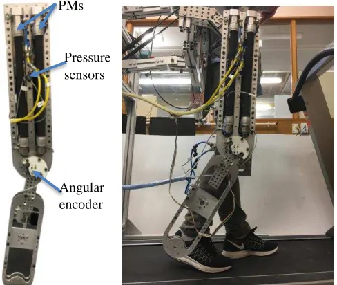
For the control algorithm development, only the knee joint mechanism of the exoskeleton is employed for the experi-mental validation. The knee joint is powered by four PM actu-ators. Each of the PM actuators is 20 mm in diameter and 300 mm in length (excluding the metal fittings in both ends). The antagonistic PMs actuate the flexion and extension of the rota-tional knee joint via 3 mm diameter steel cables with a 30 mm moment arm. Major components of the knee joint mechanism are illustrated in Fig. 1 and 2. Two 3/5 analogue valves are utilized, so the pneumatic flow of each side of the antagonistic
PMs is adjusted by one valve. Subscripts E and F are utilized to denote the parameters for the extension and flexion PMs, re-spectively. A pair of pressure sensors is also used to measure the PM pressures (PE, PF). It is assumed that all the dynamics of the two PMs to flexion/extension side are identical. An angular encoder is mounted along the joint axis to measure the angular position of the joint, , whose value is zero when the center lines of thigh and shank segments coincide and increases as the joint flexes. The interface between the electrical-pneumatic system and the PC based control platform is implemented using National Instrument MyRio. The FPGA inside MyRio is pro-grammed for hardware interfacing and signal filtering.
Fig. 1 Left: structure of the knee joint mechanism with key components an-notated; right: a healthy subject participating in a validation experiment with the mechanism
Shan k Se
gm en
t k
r PMs
for E xte
ns ion PMs
for E xte
ns ion PMs
for F lex
ion Th
igh Se
gm ent
K=0
h
Fig. 2 Schematic drawing of the PM actuated knee joint mechanism. How the angular values are calculated is also illustrated.
In terms of the kinematics, the following assumptions are made: the driving cables are always in tension and the stretch of the cables is neglected. Therefore, the contracting length of the
PMs
Pressure sensors
[image:3.612.323.567.214.420.2]PM actuators can thus be expressed by:
0 0
( )
( )
F k F E E k
x r x r
(2)
where, is the effective radius of the pulley or the joint mo-ment arm of the PM actuators; =90° and =0° are the knee joint positions when the flexor and extensor PMs have no contraction or extension, respectively. Detailed illustration can be found in the schematic drawing of Fig. 2.
B. Load Dynamics of the Mechanism
The dynamics of the knee joint mechanism can be described by the following equation.
(3)
where, is mass polar moment of inertia; is friction coeffi-cient of the actuation system which can be neglected; is the net torque provided by the antagonistic PM actuators; is the maximum joint torque produced by gravity and is angle between centerline of the thigh segment and the vertical direc-tion shown in Fig. 2. The moving mass of them PMs is less than 5% of the mass of the shank segment. Therefore, only the polar moment of inertia of the shank segment is consid-ered to determine , which can be estimated from the com-puter-aided-design of the exoskeleton.
C. Force Dynamics of the PM Actuators
Both theoretical and phenomenological models of PMs have been developed. Chou and Hannaford [20] developed a theoretical static model which links the PM’s inner pressure and contraction length to its force output. In terms of phe-nomenological models, a commonly adopted model was pro-posed by Reynolds et al. [12], in which the PM was modelled similarly to the well-known Hill’s muscle model in biome-chanics. As a dynamic model, it expresses the output force as a function of PM’s inner pressure and kinematics. This model also addresses its hysteresis behavior by applying different damping coefficients during the PM’s inflating and deflating processes.
Due to the bandwidth requirement of the robotic gait reha-bilitation system, dynamic rather than static modelling methods were considered. The dynamic model developed in [12] was modified to fit the dynamic behavior of the FESTO PM actu-ators in this application. The dynamics of a PM actuator can be expressed as:
( ) ( ) ( )
F P B P x K P x L Mx (4)
0 1 0 1 0 _ 1_ 0 _ 1_
( ) ( )
(0.6 6 )
( ) ( )
( ) ( )
i i d d
F P F F P K P K K P
P bar B P B B P Inflation
B P B B P Deflation
(5)
where, F(P), B(P), K(P) are the pressure dependent force,
damping and spring parameters, respectively (5), which are determined experimentally; M is the mass of the load; xis the
PM contracting length and Lis the force exerted on the load. These parameters are modelled linearly dependent on the inner pressurePof the corresponding PM. The damping element has different expression for the inflation and deflation processes to better describe PM’s hysteresis behavior.
The experiments were conducted at discrete pressures points ranging from 0.6 to 6 bar with 0.2 bar increments in order to acquire appropriate modelling parameters for the specific PMs used in our robot. The least square linear regression method was utilized to find the best fitting parameters. Detailed ex-perimental procedure is described in [21].
Since the model reported in [12] did not cover lower pressure range, Xing et al. [13] further developed the model in [12] by using piecewise linear functions to express the equivalent spring parameter K(P). Based on our experimental results, parameters have been obtained in the forms of both the original [12]and modified piecewise [13] models. It has been observed that the piecewise model can better represent the PM's dynamic response for the entire working pressure range [21]. The model adopted can be expressed by (6). The torque generated by the antagonistic arrangement of four PMs is calculated by (7).
D. Pressure Dynamics of the PM
It is assumed that pneumatic flow into and out of the PM is an adiabatic process [16]. Thus, the rate of change of pressure in PM can be described by the physics based model as:
( , )E F ( , )E F ( , )E F ) / ( , )E F
P RTm PV V (8)
2
( , )E F 2 1 ( , )E F 2 ( , )E F 3
V a x a x a (9)
where is the ratio of specific heats for air, R is the universal gas constant, T is the gas temperature, is the pneumatic mass flow rate of the PMs (positive for flow into the PMs) and V is the volume of air inside the PMs of each side of the antagonistic pair. V is modelled as a function of muscle contraction length (x) in (9). The regression coefficients ( , and ) of this equation are determined experimentally.
E. Flow Dynamics of the Valves
The proportional valves are modelled as dimensional com-pressible flow through an orifice. The effective area of the orifice is controlled by the voltage signal applied to the pro-portional valves. The mass flow rate is described as a function of the valve opening areas:
( ) 194.8 204.0
( ) 63382 25085 (0.6 2 ) ( ) 16352 787.9 (2 6 )
( ) 6275 946.4 ( ) ( ) 763.9 91.04 ( )
F P P
K P P P bar
K P P P bar
B P P Inflation
B P P Deflation
(6)
2 [ ( ) ( ) ( ) ( ( ) ( ) ( ) )]
F F F F F
E E E E E
r F P B P x K P x F P B P x K P x
( , )E F u, d ( , )E F ( , )E F u, d
m P P A P P (10)
1 / 1/
1 / 1 2 1 / ( ) , 1 1 ( ) u d C P f u RT
if P P C choked d u r P P
P P
d d C P
f u
RT P P
u u otherwise unchoked (11)
In the two equations above, is the equivalent valve area for the PMs on the respective side; and are the up-stream and downup-stream pressures, respectively; is the dis-charge constant and is the pressure ratio that that divides the flow into choked and unchoked flow through the orifice. Dur-ing PM inflation, equals the supply pressure of the com-pressor and equals the pressure of the corresponding PM. During PM deflation, equals the PM pressure and equals the atmospheric pressure.
III. MIMOSLIDING MODE CONTROLLER
In the previous section, the system has been modelled into four stages in series, which are the flow dynamics of the valves, the pressure dynamics and the force dynamics of the PM, and the load dynamics of the joint mechanism. By combining these models, the overall system model can be developed. The two model outputs are the knee joint position and the average pressure of the antagonistic PMs. The two inputs are the equivalent areas of the two valves. A state-space (SS) model representation was constructed for the ease of MIMO SM control implementation. The SS variables ( ), control input ( ) and output ( ), vectors are given in (12-14).
1 2 3 4
T T
k k F E
x P P x x x x (12)
TF E
u A A (13)
1( ) 2( )
1 ( 3 4) / 2
T
y y x y x x x x (14)
By combining (2) to (9), the nonlinear state-space model can be written in the form of:
( ) ( )
xf x g x u (15)
or xf x( )g x u1( )1g x u2( ) 2 (16)
0 0 2 1 0 2 1 0 2 22 ( ) ( ) ( ) /
( ) ( ) ( ) / J
si 2 ( )
n( ) /
0.5 4 2 /
0.5 4 /
k
F F k F k F E E k E k E h k
k F k k F E k k E F
E k
r F P r K P r P J
F P r P r P
B
r K
G J
P a r r V
P a r r V
B f x a a (17) 0 0 0 0 0 0 ( ) / / F F E E RT V V g x R T (18)
3 21 2 0
2 0
2 2 2
F a F k a F k
V a r r (19)
3
2
1 2 0
2 0
2 2 2
E a E k a E k
V a r r (20)
A coordinate transformation [22] is performed in (21) to make the system outputs and their derivatives as new SS vari-ables.
2
1 1 1 2 1 2 2 3 4
( ) ( ) ( ) ( ) ( )
( ) / 2
T f f
T
z x y x L y x L y x y x
x x x x x
(21)
where the expression of stands for the directional de-rivative of scalar with respect to vector f( ), which has the following properties:
1 1
( ) i ( ) ... i ( )
f i n
n
y y
L y f x f x
x x
(i1, 2) (22)
1
( ) ( )
k k f i f f i
L y L L y
(i1, 2) (23)
Based on (16), the time derivative of output is calculated in (24) and the time derivative of the new SS variable vector is calculated with (25) to (30).
1 2
1 1 2 2 1 2
( ) ( ) ( )
( ) ( ) ( )
i i i
f i g i g i
dy y x y
f x g x u g x u dt x t x
L y L y u L y u
(i1, 2) (24)
1 1
22
3 2 2
1 1 1 1 2
2 2 1 2 2
( ) ( ) ( )
( ) ( ) ( )
f g f g f
f g
k k
g
z
L y x L L y x u L L y x u
L y x L y x u L y x u
(25)
31( ) 1( ) 2( ) 3( ) 4( )
k k k k
k k F
f
E
L y x f x f x f x f x
P P
(26)
2
/ 2 E E /
k k r KF PF K P J
/
2 2
/E E k k r BF PF B P J
k/PF
2r F
F1BF1krKF1
F0k
r
/J
k/PE
2r F
E1BE1krKE1
E0k
r
J
1
2
1( ) ( k/ ) 31( ) 0
g f F
L L y x P g x (27)
2
2
1( ) k/ E 42( ) 0 g f
L L y x P g x (28)
2( )
3( ) 4( ) / 2
f
L y x f x f x (29)
1 2( ) 31( ) / 2 0
g
L y x g x ;
2 2( ) 42( ) / 2 0
g
L y x g x (30)
2
1 k kd 2 k kd k kd
(31)
2 (PF PE)/ 2 P0d
(32)
where is for the joint space trajectory; is for the average pressure;
is a tuning parameter of the sliding surface; , , are the desired knee joint angular position, velocity and acceleration, respectively; is the desired average pressure of the antagonistic PM actuators.With the selected sliding surfaces, the control law can be designed in order to drive the SS trajectories to the sliding surface. Once reached, the trajectories are forced to stay on the sliding surfaces by the controller. A classic controller design [23] is described as:
2
1
2 i i i i i d
dt
(i1, 2) (33)
in which is strictly positive. The time derivatives of (31) and (32) can be expressed in the vector form of:
1 2 1 2 2 3 1 1 2 2 2 21 1 1
2 0 2 2 ( ) ( ) ( ) ( ) ( ) ( )
k kd k kd kd f f
g f f
g g
d g
L y x
L y x
L L y x L L y x u
u u
L y x L y x P
H S Q
(34)
3
1 2 1( ) 2( ) T T
f f
h h L y x L y x
H (35)
1 2 1 2 2 2 1 1 1 23 4 2 2
( ) ( )
( ) ( )
g f g f
g g
L L y x L L y x q q
q q L y x L y x
Q (36)
2
2 0
1
T T
k kd k kd kd d
s s P
S (37)
Hence, the SM control law can be applied. The control action contains two segments:
1
( eq rob)
uQ u u (38)
where, is a continuous equivalent control element, which helps reaching of the sliding surfaces for desired motions; is the discontinuous robust element, which makes sure that the desired motions are sustained by sticking to the sliding surface. By zeroing, the expression of and can be derived as:
eq
u = -H - S (39)
1sgn( 1) 2sgn( 2)
T rob
u k k (40)
Based on (27), (28) and (30), matrix Q is non-singular. It is also necessary to note that all the modelling parameter men-tioned previously are based on ideal situations. All the uncer-tainties of the model are contained by ideal matrices H and Q. Hence, for any instant, the actual representation derivatives of
the sliding surfaces are given as:
1 2 u
H S Q
1 2 h h
H 1 2
3 4 q q q q Q (41)
where Hand Qare the instantaneous actual values of the model estimated H and Q. The estimation errors of these matrices are bounded by the known function in the following ways:
i
i i
hh H
i1, 2
(42)1
1,2,3,4 i/ i
i q q
(43)
1/ 2_ max/ _ min max
i i
q q
(44)
To ensure the control law (38) satisfy the design criteria stated by (33), Equation (38) is substituted into (41):
1
i
sgn( )i i si hi ih i ik i
(i1, 2) (45)
1 (q q1 4 q q2 3) / (q q1 4 q q2 3) 0
(46)
2 (q q1 4 q q2 3) / (q q1 4 q q2 3) 0
(47)
Hence, (45) is substituted into (33) and the following rela-tionship can be generated:
sgn( ) 1 i
i ik i i si hi ih i
(i1, 2) (48)
In order to ensure (48) is valid, needs to be selected to satisfy the following condition:
1
1
1
11 1 i
i i i i i i i i i
k s h h h (49)
Due to the use of switch functions in (40), the sys-tem is prone to high frequency chattering along the sliding surfaces. The solution to this problem is replacing the switching element along the sliding surface with piece-wise saturation function with a boundary layer [23, 24]. Hence the robust con-trol element can now be expressed as:
1(
1/
1)
2(
2/
2)
T rob
u
k sat
k sat
(50)where, is boundary layer thickness for the corre-sponding sliding surfaces.
IV. EXPERIMENTAL RESULT
with little alternation. The sampling frequency for all the sen-sors were chosen to be 1 KHz and the SM controller ran at 100Hz.
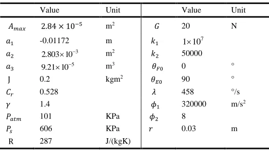
TABLE I
LIST OF PARAMETERS USED IN MODEL AND CONTROLLER IMPLEMENTATION
Value Unit Value Unit
m2 20 N
-0.01172 m 7
1 10
3
2.803 10 m2 50000 5
9.21 10 m3 0 °
J 0.2 kgm2
90 °
0.528 458 °/s
1.4 320000 m/s2
101 KPa 8
606 KPa 0.03 m
R 287 J/(kgK)
Three major parameters of the controller , ,
, together with the boundary layer width and were tuned through experimental iterations to optimize the controller performance. The tuned parameters and various modelling constants are listed in TABLE I. It is noteworthy that the equivalent area of a valve is constrained by the maximum opening area, . The applied voltage to the valve,U
i, which is the actual input to the physical system, is calculated using a linear piecewise function of the controller output , given as:max max 6
max max max max
178592 5.255 (0.02 )
10 5 ( 0.02 0.02 ) ( , )
178592 4.745( 0.02 )
i i
i i i
i i
A A A A
U A A A A i E F
A A A A
(51)
The developed and tuned multivariable SM controller has been extensively validated with a variety of experiments. All the experiments reported in this manuscript were conducted on subjects, who were healthy and had no lower limb injury. The ethics approval for experiments with healthy subjects was granted by the University of Auckland Human Participants Ethics Committee (Ref. 014970). Written consents were ob-tained from all the participants. Tracking both the knee joint trajectory and the average PM pressure is the main objective of the controller; hence this was validated primarily. When con-ducting the experiments, the subjects were asked to stand up-right with their up-right legs strapped to the shank (Figure 1). It was ensured the shank and thigh segments of the subjects’ legs and the mechanism were aligned; meanwhile the human’s and mechanism’s knees were also aligned to be coaxial. It was ensured that the human’s and mechanism’s knee joint positions were equal.
Instead of using sinusoidal reference trajectories, a healthy subject’s knee joint trajectory during level walking was adapted as the position control reference in this study. The first ex-periment conducted was to validate the main objective, which is the tracking performance of both the knee joint trajectory and the average PM pressure of the MIMO SM controller. A male
subject (Height: 178cm, weight: 75kg) participated in this experiment. The subject was instructed to relax his right leg and let the mechanism to guide the knee joint movement. The ref-erence knee trajectory was set to 5 seconds per gait cycle; meanwhile, step changes to the reference average pressure were also applied. The experimental results are shown in Fig. 3. The figure indicates both the trajectory and pressure tracking were effective. The controller was tuned so that the step changes of the desired average pressure can be reacted quickly enough without affecting the trajectory control performance. This tuning setup resulted a longer rising time, but no overshoot in the average pressure when the reference changed from 200 KPa to 320 KPa and then to 360 KPa. Such controller behavior is thought to be acceptable, as sharp changes in compliance level are unlikely to happen during robotic rehabilitation training. It is observed that the trajectory control accuracy increased as the average pressure increased, which also indicates a decrease in the actuators’ compliance.
[image:7.612.327.546.277.462.2]ments are illustrated in Fig. 4.
The three subplots (A, C and E) in the left column of Fig. 4 are for the first group of experiments. The subplots (B, D and F) in the right columns are for the second group. The periods when the subjects were requested to obstruct are highlighted in yel-low. The plots in the top, middle and bottom rows are of ex-periments when the average PM pressure was regulated to 360, 270 and 180KPa respectively.
From Fig. 4(A, C and E), it can be observed that the MIMO SM controller is capable of tracking the desired knee joint trajectory at different average PM pressures with different subjects. The tracking accuracy decreases with the average PM pressure. Such changes in tracking accuracy could be inter-preted as a result of changes in compliance. Such interpretation was validated in the second group of experiments whose results are shown in Fig. 4 (B, D and F).
In Fig. 4(B), only small increase in trajectory deviation is observed compared to Fig. 4(A), during the period when the subjects obstructed the mechanism’s guidance. This means that the mechanism’s joint had a low level of compliance when the average PM pressure was regulated at 360 KPa. When the average PM pressure was reduced to 270 KPa, an increase in trajectory deviation appeared during the obstructing periods, as shown in Fig. 4(D). This indicates a rise in compliance, and the subjects had more freedom around the desired trajectory. There was a further increase in compliance as the average PM pres-sure was reduced to 180KPa. At this prespres-sure, the subjects could back-drive the mechanism to much further positions away from its reference. The behavior of controlled actuators’ intrinsic compliance while performing trajectory tracking is comparable to controllers that simulate variable impedance or
virtual tunnels along a desired trajectory on motor driven gait rehabilitation exoskeletons [25, 26].
The final experiment was designed to explore the bandwidth of the SM controlled system. As mentioned in the introduction section, the gait rehabilitation training needs to be task specific. Hence, the controller and the hardware system need to be able to operate at a bandwidth that is similar to the average gait cycle frequency (0.67Hz) of stroke survivors [27]. The experiment was conducted with the same male subject and with the same setup as those of the first experiment. During the experiment, the subject was instructed to relax his right leg and let the mechanism guide the knee joint movement at discrete fre-quencies varying from 0.2 to 0.7 Hz with 0.1 Hz increment. The average PM pressure was regulated at 360 KPa for this ex-periment. The experimental result is shown in Figure 5. It can Fig. 4 Results of the experiments on knee joint trajectory tracking and compliance control with five healthy subjects. (A) (C) (E): the subjects were instructed to relax their right knees during the entire experiments; (B) (D) (F): the subjects were instructed to obstruct the mechanism’s guidance during the time period high-lighted in yellow. Average PM pressure was regulated at 360, 270 and 180 KPa for the results plotted in top (A, B), middle (C, D) and bottom (E, F) rows, respec-tively.
(D) (B) (A)
(C)
be seen that the control system is stable and effective at all the frequencies, although the trajectory tracking performance worsens as demonstrated by an increase in the RMS trajectory error with the frequency. One major contribution of the in-crease in RMS trajectory error is the inin-crease in the phase delay between the actual and desired trajectory, which could be caused by the intrinsic compliance of the PM actuation system, although, the compliance was controlled to a low level during the experiment.
V. CONCLUSIONS
The paper proposed a new MIMO SM control on a PM ac-tuated robotic mechanism. Experimental results demonstrated that both reference joint angular trajectory and average PM pressure can be tracked effectively and simultaneously.
In terms of SM controller implementation, non-integral ra-ther than integral sliding surfaces were adapted, although in-tegral control surfaces might lead to better trajectory tracking performances. The reason for such a decision is the safety of future gait rehabilitation applications of the system. During rehabilitation training, the active input of a subject may result in the accumulation of trajectory errors. Controller with integral sliding surfaces may react to the accumulation of trajectory errors with sudden movement or a short period of high fre-quency oscillation. This may cause discomfort or even injuries to the subject.
Further work will be design and implementation of a gait assessment module that provides reference compliance or av-erage pressure to the MIMO controller in order to adjust the assistance level of the gait rehabilitation training.
REFERENCES
[1] D. P. Ferris, J. M. Czerniecki, B. Hannaford, U. of Washington, and V. P. S. H. System, "An ankle-foot orthosis powered by artificial pneumatic muscles," Journal of Applied Biomechanics, vol. 21, p. 189, 2005. [2] G. S. Sawicki and D. P. Ferris, "A pneumatically powered
knee-ankle-foot orthosis (KAFO) with myoelectric activation and inhibition," J Neuroeng Rehabil, vol. 6, p. 23, 2009.
[3] T. G. Sugar, J. He, E. J. Koeneman, J. B. Koeneman, R. Herman, H. Huang, et al., "Design and control of RUPERT: a device for robotic upper
extremity repetitive therapy," IEEE Trans. Neural Syst. Rehabil. Eng., vol. 15, pp. 336-346, 2007.
[4] S. Hussain, S. Q. Xie, P. K. Jamwal, and J. Parsons, "An intrinsically compliant robotic orthosis for treadmill training," Med. Eng. Phys., vol. 34, pp. 1448-1453, 2012.
[5] D. G. Caldwell, G. A. Medrano-Cerda, and M. Goodwin, "Control of pneumatic muscle actuators," IEEE Control Systems, vol. 15, pp. 40-48, 1995.
[6] P. Carbonell, Z. Jiang, and D. Repperger, "Nonlinear control of a pneumatic muscle actuator: backstepping vs. sliding-mode," in Control Applications, 2001.(CCA'01). Proceedings of the 2001 IEEE International Conference on, 2001, pp. 167-172.
[7] S. W. Chan, J. H. Lilly, D. W. Repperger, and J. E. Berlin, "Fuzzy PD+I learning control for a pneumatic muscle," in Fuzzy Systems, 2003. FUZZ '03. The 12th IEEE International Conference on, 2003, pp. 278-283 vol.1. [8] T. D. C. Thanh and K. K. Ahn, "Nonlinear PID control to improve the control performance of 2 axes pneumatic artificial muscle manipulator using neural network," Mechatronics, vol. 16, pp. 577-587, 2006. [9] J. Huang, J. Qian, L. Liu, Y. Wang, C. Xiong, and S. Ri, "Echo state
network based predictive control with particle swarm optimization for pneumatic muscle actuator," J. Franklin Inst., vol. 353, pp. 2761-2782, 2016.
[10] M. Van Damme, B. Vanderborght, R. Van Ham, B. Verrelst, F. Daerden, and D. Lefeber, "Proxy-based sliding mode control of a manipulator actuated by pleated pneumatic artificial muscles," in IEEE Int Conf Robot Autom, 2007, pp. 4355-4360.
[11] J. H. Lilly and L. Yang, "Sliding mode tracking for pneumatic muscle actuators in opposing pair configuration," IEEE Trans. Control Syst. Technol., vol. 13, pp. 550-558, 2005.
[12] D. Reynolds, D. Repperger, C. Phillips, and G. Bandry, "Modeling the dynamic characteristics of pneumatic muscle," Ann. Biomed. Eng., vol. 31, pp. 310-317, 2003.
[13] K. Xing, J. Huang, Y. Wang, J. Wu, Q. Xu, and J. He, "Tracking control of pneumatic artificial muscle actuators based on sliding mode and non-linear disturbance observer," IET control theory & applications, vol. 4, pp. 2058-2070, 2010.
[14] M.-K. Chang, "An adaptive self-organizing fuzzy sliding mode controller for a 2-DOF rehabilitation robot actuated by pneumatic muscle actuators," Control Eng. Pract., vol. 18, pp. 13-22, 2010.
[15] T.-Y. Choi, B.-S. Choi, and K.-H. Seo, "Position and compliance control of a pneumatic muscle actuated manipulator for enhanced safety," Control Systems Technology, IEEE Transactions on, vol. 19, pp. 832-842, 2011. [16] X. Shen, "Nonlinear model-based control of pneumatic artificial muscle
servo systems," Control Eng. Pract., vol. 18, pp. 311-317, 2010. [17] H. Aschemann and D. Schindele, "Sliding-mode control of a high-speed
linear axis driven by pneumatic muscle actuators," IEEE Trans. Ind. Electron., vol. 55, pp. 3855-3864, 2008.
[18] A. Sala, Multivariable control systems an engineering approach. London: London : Springer c2004., 2004.
[19] J. Cao, S. Q. Xie, R. Das, and G. L. Zhu, "Control Strategies for effective robot assisted gait rehabilitation: The state of art and future prospects," Med. Eng. Phys., vol. 36, pp. 1555-1566, 2014.
[20] C.-P. Chou and B. Hannaford, "Measurement and modeling of McKibben pneumatic artificial muscles," IEEE Transactions on Robotics and Automation, vol. 12, pp. 90-102, 1996.
[21] J. Cao, S. Q. Xie, M. Zhang, and R. Das, "A New Dynamic Modelling Algorithm for Pneumatic Muscle Actuators," in Intelligent Robotics and Applications, ed: Springer, 2014, pp. 432-440.
[22] M. Smaoui, X. Brun, and D. Thomasset, "Systematic control of an electropneumatic system: integrator backstepping and sliding mode control," IEEE Trans. Control Syst. Technol., vol. 14, pp. 905-913, 2006. [23] J.-J. E. Slotine and W. Li, Applied nonlinear control vol. 199:
Prentice-Hall Englewood Cliffs, NJ, 1991.
[24] K. D. Young, V. I. Utkin, and U. Ozguner, "A control engineer's guide to sliding mode control," IEEE Trans. Control Syst. Technol., vol. 7, pp. 328-342, 1999.
[25] S. K. Banala, S. K. Agrawal, S. H. Kim, and J. P. Scholz, "Novel Gait Adaptation and Neuromotor Training Results Using an Active Leg Exoskeleton," IEEE/ASME Trans. Mechatron., vol. 15, pp. 216-225, 2010.
[26] A. Duschau-Wicke, J. von Zitzewitz, A. Caprez, L. Lunenburger, and R. Riener, "Path Control: A Method for Patient-Cooperative Robot-Aided Gait Rehabilitation," IEEE Trans. Neural Syst. Rehabil. Eng., vol. 18, pp. 38-48, Feb 2010.
FGC (Hz) 0.2 0.3 0.4 0.5 0.6 0.7
ERMS (°) 3.11 6.32 7.42 9.10 11.39 11.79
Fig. 5 Knee joint trajectory versus gait cycle progress plots at different gait cycle frequencies (FGC). The RMS trajectory errors during two gait cycles are