(will be inserted by the editor)
A State-Space Model and Control of a Full-Range PMSG Wind Turbine
for Real-Time Simulations
Agust´ın Tob´ıas-Gonz´alez1 · Rafael Pe ˜na-Gallardo1 · Jorge Morales-Salda ˜na1 · Aurelio Medina-R´ıos2 · Olimpo Anaya-Lara3
Received: 10/11/2017 / Accepted:
Abstract Direct drive permanent magnet synchronous ge-nerators (PMSG) have drawn great interest to wind turbine manufacturers, due to the advance of power electronic tech-nology, improved designs and fabrication procedures of these types of generators. In this research, a state-space model of a PMSG wind turbine was developed, and used for the obtain-ment of a control strategy in a easier way for a test system in thedqreference frame. Then, a complete model of a PMSG wind turbine connected to an electric grid through a full-scale Back-to-Back (BTB) converter with its controls was implemented, using the detailed models included in a Real-Time Digital Simulator (RTDS). Simulation results show that the controllers perform efficiently during transient and steady state conditions, and that the presented model can be used for the development of control strategies prior to their implementation in a professional software.
Keywords Control Strategies·Modeling and Simulation· Real Time·Synchronous Generator·Variable Speed Wind Turbine.
1 Introduction
Wind power is today’s most rapidly growing renewable ener-gy source. Wind turbines can either operate at fixed speed or
Rafael Pe˜na-Gallardo [email protected]
1Facultad de Ingenier´ıa, Universidad Aut´onoma de San Luis Potos´ı,
San Luis Potos´ı, M´exico
2 Facultad de Ingenier´ıa El´ectrica, Universidad Michoacana de San
Nicol´as de Hidalgo, Morelia, M´exico
3 Institute for Energy and Environment, University of Strathclyde,
Glasgow, UK
variable speed. In a fixed-speed wind turbine, the generator, normally a conventional squirrel-cage induction machine is directly connected to the grid through a transformer [1–3]. Variable speed wind turbines are controlled by power elec-tronic equipment, and depending on the arrangement, both induction and synchronous machines can be employed [4– 7].
Recently, the concept of a variable-speed wind turbine equipped with permanent magnet synchronous generators (PMSG) has received increased attention by various wind turbine manufacturers. The use of permanent magnets in the rotor of the PMSG makes unnecessary to supply magne-tizing current through the stator for constant air-gap flux; the stator current needs to be only torque producing [8, 9]. Hence for the same output, the PMSG can operate at a higher power factor because of the absence of magnetizing current, and will be more efficient than the induction machine used in other types of wind turbines.
Several models that represent the dynamic behavior of the PMSG wind turbine have been reported in the open lit-erature. Most of them are formulated in the phase domain [10], since in this frame the dynamics of the PMSG wind turbine can be represented in a natural way. For instance, re-cently in [11] a dynamic model of a PSMG wind turbine is proposed for small capacity turbines, while in [12] the dy-namic modeling and control of a PMSG wind turbine with MPPT control connected to the grid is presented. However, phase domain models have the disadvantage that the compu-tational load involved in their solution is high, and because of this, they are not suitable for real-time simulations [13].
the modeling [4, 15]. In this contribution a state-space model in thedqreference frame was developed based on these con-siderations, that is, the model needs to be simpler compared with models obtained in the phase domain and preserve the dynamic behavior of the test system. The developed model meets these characteristics and includes the modulation sig-nal required to control the power electronic converter, that allows the link between the wind turbine and the grid; varia-ble that is omitted in many works.
On the other hand, various techniques have been de-veloped to investigate the behavior of a PMSG wind tur-bine under differentdqcontrol conditions [16–19]. The most widely used control technique is the linear control based on the proportional integral derivative (PID) technique, since it is robust, simple and easy to implement [20]. Nonlinear control has been also used for the control of wind turbines; the most popular technique is the sliding mode control [21]. This technique has the advantage to be robust and provides dynamic invariant property with uncertainties, however this technique presents the chaterring phenomenon [22]. Alter-native control techniques based on intelligent algorithms also have been proposed for the control of wind turbines, such as neural networks [23, 24], and fuzzy control [25]. Another type of control reported in the literature is the predictive control; this technique is used to represent the behavior of complex dynamic systems using estimation models [26].
Regarding to the control strategy developed in this con-tribution, a linear control strategy was used for the PSMG wind turbine, because the computational effort is low, it can be used for real-time simulations and performs well under different scenarios.
The state-space model of a PMSG wind turbine pre-sented in this paper includes a full-scale BTB converter for its connection with an electric grid, for the study and obtain-ment of a full-control strategy. The impleobtain-mentation of the model was done in the C programming language, the model was designed to be included as part of the main component library of the graphical user interface of a Real-Time Digi-tal Simulator (RTDS) [27]. This model can be connected to other customized component model libraries included in the RSCAD software. The controllers were programmed in a digital device, using the Rapid Control Prototyping (RCP) technique [28], with the aim to explore the system perfor-mance in real-time [29, 30].
The rest of this paper is organized as follows: Section 2 presents a description of the structure and the modeling of the test system; Section 3 presents the PMSG wind turbine model developed in this research; Section 4 shows control strategies used in the converter in order to obtain the maxi-mum power extraction of the wind turbine; Section 5 con-tains the tuning technique used in the controllers; Section 6 describes the RTDS station used in this investigation, as well as some considerations taken into account at the moment of
the implementation of the wind turbine model and the con-trol strategy using the RCP technique; in Section 7 simula-tions of the PMSG wind turbine model connected to an elec-tric grid through a electronic converter during transient con-ditions are presented and discussed; finally, Section 8 draws the main conclusions of this work.
2 Structure and modeling of the test system
Fig. 1 illustrates the general structure of a PMSG wind tur-bine connected to grid. The system consists of the following elements [31, 32]:
a) A wind turbine including a stochastic model that repre-sents a wind sequence.
b) A standard permanent magnet synchronous machine, with the stator windings connected to the grid through a full-scale frequency converter.
c) A model of a grid.
CA
CD CA
CD
β
PMSG BTB converter Wind
turbine Wind
model Grid model
3ϕ
∆-Y VSC1 VSC2
Fig. 1 PMSG wind turbine.
2.1 Wind model
This model represents the behavior of the wind as a speed sequence, and it has the advantage of cover a full range of characteristics of a real wind sequence. The model is com-posed by the sum of four components [33]:
vw(t) =vavg+vr(t) +vg(t) +vt(t), (1)
wherevavg is the average value of the wind speed (m/s),
vr(t)is the ramp component (m/s),vg(t)is the gust
com-ponent (m/s), andvt(t)is the turbulence component of the
wind (m/s), which is defined by Eq. (2) [33].
vt(t) = n
∑
i=1p
Swt(fi)∆f cos(2πfit+φi+∆ φ) (2)
Where fi is the frequency ofi−thcomponent (Hz),φi
is the phase of the same component (rad),his the height to the shaft level (m),lis the turbulence length (m), andz0is
Swt(fi)is the power spectrum (W/Hz), given by the Eq. (3),
established in the Danish standard[34].
Swt(fi) = 1
(ln(h/z0))2lvavg
(1+1.5vavgfil )53
(3)
2.2 Aerodynamic model
There are many mathematical models that have been ob-tained to describe the relationship between the wind speed and the mechanical power extracted from the wind [35, 36]. This paper uses the following equation to model a wind tur-bine:
Pw=
ρ
2ArCP(λ,β)vw
3 (4)
wherePw is the extracted power from the wind,ρ is the air
density (kg/m3),Ar is the area covered by the wind turbine
rotor (m2),v
w is the wind speed (m/s), andCpis the power
coefficient which is a function of both tip speed ratioλ, and
blade pitch angleβ (rad). To calculateCpfor the given
va-lues ofβ andλ the following numerical approximation has
been used [37].
CP(λ,β) =c1( c2
λi
−c3β−c4)e (−c5
λi)+c
6λ (5)
λi=
( 1
λ+0.08β)−(
0.035
β3+1) −1
(6)
The values of the coefficientsc1-c6are dependent of the
wind turbine design. In this research the following values were used:c1=0.5176,c2=116,c3=0.4,c4=5,c5=21
and c6=0.0068. Fig. 2 shows curves ofCp for different
wind speed values. Each curve shows a maximum point that corresponds to the maximum power that can be extracted from the wind.
Turbine output power (
pu
of
nominal mechanical power)
Turbine speed (pu of nominal generator speed) Máximum power at base wind
speed (11.5 m/s) and β=0°
5 m/s
7.6 m/s 6.3 m/s
8.9 m/s 10.2 m/s
11.5 m/s 12.8 m/s
Fig. 2 Wind turbine power characteristics withβ=0◦.
2.3 Torque equation
The torque equation describing the mechanical behavior of the wind turbine can be written based on a single-mass model given as [33, 38]:
Te=
2J P
d dtωr+
2Bm
P ωr+TL (7)
whereTL is the average aerodynamic torque (N·m), Te is
the electromagnetic torque (N·m),Jis the inertia constant of the wind turbine and the generator (kg·m2),ωr is the
frequency of the generator rotor (rad/s),P is the number of poles of the machine, and Bm is a damping coefficient
associated with the rotational system of the machine and the mechanical load (N·m·s).
2.4 Generator model
The generator was modeled considering the following assump-tions:
– Magnetic saturation is neglected.
– Any losses, apart from copper losses, are neglected. – The flux distribution in the windings is considered to be
perfectly sinusoidal.
The voltage equations of a permanent magnet synchronous generator in thedqsynchronous reference frame can be ex-pressed as [38]:
vdrs =Rsidrs +Ld
d dti
dr
s +ωrLqisqr+ωrλm0r (8)
vqrs =Rsiqrs +Lq
d dti
qr
s −ωrLdidrs (9)
wherevd,qs are the voltages (V), Rs is the resistance (Ω), id,qs are the currents (A),Ld,qare the inductances of the
sta-tor (H), andλm0r is the flux of the permanent magnet (Wb).
Thessubscript denotes variables and parameters associated with the stator circuit andrsubscript is associated with ro-tor variables; thedqsuperscript stands for variables in the synchronous reference frame.
The electromagnetic torqueTedeveloped by the machine
(N·m) can be obtained from the following equation [39]:
Te=
3P 4
h
λm0ridrs + (Lq−Ld)idrs iqrs
i
(10)
2.5 Full-scale BTB converter model
[image:3.595.41.279.592.715.2]Fig. 3 shows a PMSG wind turbine with a two-level full-scale BTB converter selected for the connection of the wind turbine to the grid. This topology gives the advantage of in-creasing the degrees of freedom in the system, where the V SC1controls the active and reactive power provided by the
PMSG and theV SC2controls the regulation of the DC-link,
and the reactive power at the Point of Common Coupling (PCC) [40, 41].
Vdc
Two-level Back-To-Back PWM-VSC PMSG Wind
Turbine
3ϕ
∆-Y Grid model
β
Fig. 3 BTB converter topology.
The dynamic model for the BTB converter [40] is ob-tained in order to have a full dynamic model of the system, and design the control strategies.
3 Full dynamic model of a PMSG wind turbine including a BTB converter
Taking into account the Eqs. (7)-(10) and the model of the BTB converter shown in the Fig. 3 [40], a state-space model of the PMSG wind turbine was obtained.
Equations (11)-(16) show the state-space dynamic model for the PMSG wind turbine including a BTB converter de-veloped in this research. This model is helpful for the design and analysis of different control strategies; besides, it repre-sents the dynamic behavior of the complete system and can be used in different type of studies.
d
dtωr=−
Bm
J ωr+
3P2
λm0
8J i
d
1−
P
2JTL (11)
d
dti
d
1= [
1
L1−Ld
][(Rs−R1)id1+ (L1+Lq)ωriq1+λm0ωr−
md1vcd
2UT1
] (12)
d
dti
q
1= [
1
L1−Lq
][(Rs−R1)iq1−(L1+Ld)ωrid1−
mq1vcd
2UT1
] (13)
d
dti
d
2=−
R2
L2
id2+ω2iq2+
vd
2
L2
− m
d
2vcd
2UT2L2
(14)
d
dti
q
2=−
R2
L2i
q
2−ω2id2+
vq2
L2−
mq2vcd
2UT2L2
(15)
d
dtvcd=
3
2CcdUT1
(md1id1+mq1iq1) + 3
2CcdUT2
(md2id2+mq2iq2) (16)
Eq. (11) represents the shaft model including the elec-tromagnetic torque; Eq. (12) and (13) represent theV SC1;
Eq. (14) and (15) represent theV SC2; and Eq. (16)
repre-sents the dynamic of the DC-link voltage. Besides,vdi and
vqi are the voltages,id,qi the line currents,Ri andLiare the
resistance and the inductance of theV SCi, respectively,vdc
the voltage in the DC-link,md,qi is the signal of modulation andUTi the maximum value of the triangular wave for the
Pulse-Width Modulation (PWM).
It is important to mention that this developed model is used to obtain the control techniques for the wind system, then these techniques were tested using the detailed models included in RSCAD and the results show that they work well and were obtained using a simplified model in an easier way.
4 Control strategies of the BTB converter
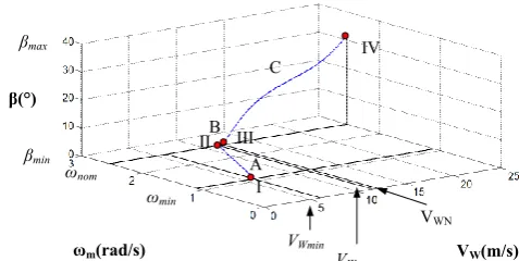
The design of the control strategies considers the operation of the variable speed wind turbine within three regions, which allow an optimal power extraction on a wide range of wind values, with a safe and optimal operation for the system.
Fig. 4 describes three basic operating regions of a varia-ble speed wind turbine [42], where the region A is the opera-tion on a low wind speed profile (LWS). In this region the value of the wind speed is below the rated value and it is necessary to operate the wind turbine at an optimal speed, trying to extract the maximum power from the wind (see Fig. 2). This is achieved by keeping the tip speed ratio at an optimal value, that is, λ =λopt, and the pitch angle at
a minimum constant value ofβ =β0. The region B is the
transition region between region A and C, where the sys-tem must have a smooth operation in order to avoid sudden mechanical vibrations that can damage the turbine. The ope-ration of the wind turbine in a wind speed above of the rated value or at high wind speeds (HWS) is carried out in the region C, where the mechanical speed must not exceed the design value of the wind turbineωm=ωnom, and also it has
to deliver its nominal electrical power to the network; this is achieved using the pitch angle control.
ωmin
VW(m/s) ωnom
ωm(rad/s) β(°)
βmax
βmin
VWωnom
I II III
IV
VWmin VWN
A B
C
Fig. 4 Operating regions of a variable speed wind turbine.
For the operating regions mentioned above in this re-search the following control objectives have been selected:
[image:4.595.48.278.208.289.2] [image:4.595.44.281.541.705.2] [image:4.595.300.539.554.674.2]– Mitigation of mechanical loads. – Keep the power quality.
In this paper, the direct drive PMSG concept is adopted with the utilization of fully-controlled power converters. The BTB converter assembly consists of a generator side AC/DC converter, a DC-link capacitor, and a grid side DC/AC con-verter. Each of the two power converters is composed of a two-level PWM-VSC converter.
The design of the control strategy of the PMSG wind turbine is based on the dynamic model given by the Eqs. (11)-(16). Fig. 5 shows the control scheme that considers the operation of the wind turbine in the LWS and HWS re-gions, whereωmppt is the optimal speed when the wind
tur-bine operate bellow the rated wind speed, and in the HWS region prevails the operation of the pitch angle controller to maintain the shaft speed at its nominal value.
WT
ω*m
Wind model
β
MPPT
ωm
PWM
VW
Wind speed (m/s)
Pm
Pitch control
ωnom βd
Vdc & Q control PMSG
+- dqabc
ωmppt
dqabc
BTB converter
PWM
Vdc
∆-Y
Grid model
+
-FOC Low wind
speed FOC High wind
speed θr 2MW, 0.69 kV L-L
0.69 kV/230 kV 3ϕ
3ϕ
θgrid
3ϕ
Load 1 MW S1
Fig. 5 Diagram of the PMSG wind turbine control [43].
4.1 Obtaining of the MPPT reference
The reference given for the maximum power point tracking algorithm (MPPT) is obtained from a function of the maxi-mum points of theCpcurves, shown in Fig. 2, and described
by Eq.(17).
ωmppt=0.0000321v3w+0.0003950v
2
w+0.2060213vw+0.076506 (17)
Appling thedqtransformation in the rotating reference frame, the active and reactive power generated by the wind turbine are given by:
P=3
2(v
qiq+vdid) (18)
Q=3
2(v
qid−vdiq) (19)
If the reference frame is such thatvq=0 andvd=|v|,
the equations for the active and reactive power are,
P=3
2(v
did) (20)
Q=3
2(v
diq) (21)
Therefore, the active and reactive powers can be con-trolled by means of the direct and quadrature current com-ponents, respectively.
4.2 Generator-side converter control
The Field Oriented Control (FOC) is used as the control technique for the converter of the generator-side. The FOC scheme proposed in this paper is shown in the Fig. 6. As this converter is directly connected to the PMSG, a mechanical speed reference given from a Maximum Power Point Algo-rithm (MPP) ωmppt is needed to determine the maximum
power extraction from the wind.
iq 1
ω* mppt
ωm
PI 0
PI
2UT1ωrλm
2LTdUT1ωr
V*cd
Σ
Σ
θr mabc
1
md 1 PI
-+ +
-+ id
1
id 1ref
iq
1ref
dq abc
-+ V*cd
2LTqUT1ωr
V*cd
mq 1
Fig. 6 Control block diagram of generator-side converter.
The active power can be controlled by means of theid
current, as described in Eq. (20). The angleθr, for the
trans-formation betweenabcanddqvariables is calculated from the rotor speed of the PMSG.
The Control Law for the FOC can be described by the following equations:
md1=2UT1
Vdc∗
(Rs−R1)id1+LT dωriq1+ωrλm0r
−U11 (22)
mq1=2UT1
Vdc∗
(Rs−R1)i1q−LT qωrid1
−U12 (23)
whereU11 andU12 are PI controllers, and the decoupling
terms areLT dωriq1andLT qωrid1.
Considering the closed loop for the id current, the PI control equation is:
U11=Kp11(id1re f−id1) + Ki11
s (i
d
1re f−id1) (24)
and the transfer function for the closed loop is obtained by substituting Eq. (22) into Eq. (12):
G11(s) =
id1(s)
id1re f(s)=
Vcd∗(Kp11s+Ki11)
2UT1(L1−Ld)s2+Kp11Vcd∗s+Ki11Vcd∗
[image:5.595.300.522.288.437.2] [image:5.595.47.285.317.417.2]4.2.1 Speed control loop
The outer loop that sends the referenceid1re f is obtained from Eq. (11), where it is considered thatBm=0 andTLis a
per-turbation, resulting in the control scheme shown in Fig. 7.
ω*mppt
PI -+
ωm
3P2λm
8J
1
s id1ref
Fig. 7 Speed control.
The closed loop transfer function is:
Gω(s) =
ωm
ωmppt∗
= 3P
2λ0
m(Kpωs+Kiω) 8Js2+3P2λ0
m(Kpωs+Kiω)
(26)
4.3 Load-side converter control
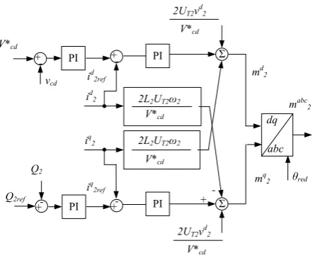
The control objectives for the load-side converter are to regu-late the DC-link voltage and to control the reactive power exchange with the network. The control strategy used in the grid-side of the inverter is the Decoupled Current Control (DCC). This technique allows to have an independent con-trol of the currents in thedqsynchronous reference frame.
The control law for the DCC can be described by the following equations:
md2=2UT2
Vdc∗
L2ω2iq2+v d 2
+U21 (27)
mq2=2UT2
Vdc∗
−L2ω2id2+v q 2
+U22 (28)
whereU21 andU22 are PI controllers and the decoupling
terms areL2ω2iq2andL2ω2id2.
Control blocks for the load-side converter with the DCC strategy are shown in Fig. 8. The control scheme consists in two inner control loops for thedqcurrents and two outer loops that send the current reference need to meet the control objectives.
In the same way than the FOC, the closed loop transfer function in the inner control loop is obtained by substituting Eq. (27) in Eq. (14).
4.3.1 DC-link control
The transfer function for the outer closed loop that sends the id
2reference is obtained by considering the steady state
ope-ration, i.e. the Eq. (16) with dtdid2=0, a unity power factor
V*cd
vcd
PI
PI
2L2UT2ω2
V*cd
Σ
Σ
θred
mabc 2
md 2
PI
-+ +
-+ id
2ref
dq
abc
-+
PI
-+ Q2
2UT2vd2 V*cd
iq 2ref
Q2ref
2L2UT2ω2
V*cd
V*cd 2UT2vd2
mq 2
id 2
iq 2
Fig. 8 Control block diagram of grid-side inverter.
withQ2=0 and a PI controller, resulting in the following
transfer function for the DC-link control:
Gcd=
vcd(s)
Vcd∗(s)=
vd
2(Kpcds+Kicd) 3
2V
∗
cdCcds2+Kpcdv d
2s+Kicdv d 2
(29)
4.3.2 Reactive power control
The reactive power control is carried out from Eq. (21); its loop control sends theiqreference to both converters. The closed loop transfer function with a PI controller is given as:
GQi=
Qi(s)
Q∗i(s)=
vdi(Kpi1s+Kii2)
(23−Kpi1v
d
i)s−Kii2v d 1
(30)
4.4 High wind speed control
Control objectives in the HWS region are to limit the me-chanical speed when the wind speed exceeds its nominal valuevwnom, and to send the nominal power to the grid. These
objectives are met by using a pitch angle controller that takes into account the mechanical power limit of the wind turbine, the nominal speed of the mechanical system, and the pitch angle required to maintain these parameters within limits.
The control scheme for this purpose is shown in the Fig. 9, which has two control loops, one for the nominal speed and other for the nominal mechanical power, it also has a time constantτof the pitch actuator.
The transfer function for the pitch angle control is given as:
Gβ(s) =
(Kpβ+Kpp)τs 2+ (K
iβτ+Kpβ(Kpp+1) +Kpp(Kpβ+1))s+2KiβKpp+Kiβ
τ2s3+ (τ+τ(K
pβ+1))s 2+ (K
pβ+Kiβτ+1)s+Kiβ
[image:6.595.308.531.95.277.2] [image:6.595.45.272.181.235.2]Σ
PI
ωnom 1
1 + sτ
ωm
βd β
βmax
βmin
dβmax
min
dβ
max Pm
Pnom
P
Σ
--
ΣFig. 9 Control scheme for the pitch angle.
5 Tuning control loops
Since the control strategies for the BTB converter contain cascade control loops, for tuning a inner control loop, it is necessary to select a bandwidth below of the switching fre-quency. For instance the criteria used on [44] is a frequency ratio ofzT =
fswi fi ≥9.
5.1 Tuning cascade loops of FOC
The switching frequency for the converter at the generator-side is selected with a modulation indexmf =81 for f1=
24.54 Hz, resulting in fsw1=1,987 Hz. The inner loops
are tuned first setting the proportional gain with a value of kp11=0.009 and for a bandwidth required, with the integral
gain selected aski11=0.0001, where its frequency ratio is zT =13. On the other hand, the proportional and integral
gains for the bandwidth of the outer speed loop are selected by using a second order system:
s2+2ζ ωns+ωn2 (32)
and consideringωn=2.57 rad/s andζ =0.59 for an
per-centage overshootPO=10 %, the result is:
Kpω=
16Jζ ωn
3P2λ0
m
=4.66 (33)
Kiω= 8Jωn2
3P2λ0
m
=10.139 (34)
The closed loop frequency response is shown in the bode diagram of the Fig. 10 withzT =63.
−40 −20 0
Magnitud
e
(dB)
10−3 10−2 10−1 100 101 102 103 104
−90 −60 −30
Ph
ase (
deg
)
Frequency (Hz)
G11(s) Gw(s) (2.27,−3)
[image:7.595.47.273.83.186.2](145,−3.02)
Fig. 10 Frequency response of cascade loops in the FOC.
5.2 Tuning cascade loops of DCC
The cascade loops of DCC are tuned in the same way that the FOC, with f2=60 Hz and fsw2 =4,860 Hz, resulting
in the following gains for the inner loops and the DC-link, respectively:kp21=0.0018 andKi21 =0.0003; Kpcd =2.0
andKicd =9.0. The frequency response is shown in Fig. 11.
10-2
10-1
100 1
102
103
104
−90 −60 −30 0
Ph
ase (deg)
10
Frequency (Hz)
−40 −20 0
Magnitud
e
(dB)
G21(s) Gdc(s)
(6.28,−3)
[image:7.595.297.537.200.315.2](113,−3)
Fig. 11 Frequency response of the cascade loops of the DC-link and the inner current loop.
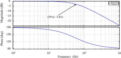
5.2.1 Tuning the reactive power loop
The reactive power loop considers tuning the PI controller with the grid frequency, and the bandwidth with a value of a decade away from the previous inner loop; this is achieved with the following expression:
KiQ =
ωc
3vd 2
v u u t
10−103 (−3Kp Qv
d
2+2)2−(3KpQv d 2)2
1−10−103
(35)
Consideringωc=377 rad/s,KpQ=0.0001, and the
nega-tive sign for the Routh-Hurwitz criteria resulting inKiQ =
−0.4059, the frequency response for the reactive power loop of the DCC is shown in Fig. 12.
100 101 102 103
90 120 150 180
Phase (deg)
Frequency (Hz) −20
−15 −10 −5 0
Magnitude (dB)
GQ2(s)
(59.6,−3.01)
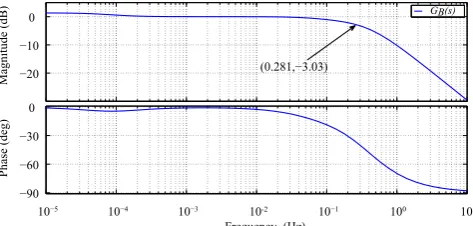
[image:7.595.298.536.600.715.2] [image:7.595.42.279.634.717.2]5.3 Tuning the pitch angle control loop
This loop takes into count an arbitrary time constant of the actuator of the bladesτ=2.5 s. By using the principle of su-perposition, the upper loop is tuned in a decade below from the speed loop with Kpβ =5.0 and Kiβ =0.003, then the
lower loop sets the gain of the closed loop to an unit gain with the proportional gain of the controller of Kpp=0.2,
resulting in the frequency shown in Fig. 13.
10−5 10−4 10−3 10−1 100 101
−90 −60 −30 0
Phase (deg)
10-2 Frequency (Hz) −20
−10 0
Magnitude (dB)
GB(s)
(0.281,−3.03)
Fig. 13 Frequency response of the pitch control loop.
5.4 HWS operation
The proposed tuning of controllers in the LWS region may have an oscillatory response when the wind turbine operates in the HWS region. To overcome this possible problem, the proportional gains of the inner loops in the FOC are set to Kp11h=Kp12h=0.0045. The frequency response for these
gains are shown in the bode diagram of Fig. 14.
−20 0
Magnitude (dB)
10−3 10−2 10−1 100 101 102 103 104
−90 −60 −30
Phase (deg)
Frequency (Hz)
G12(s)
[image:8.595.310.536.79.216.2](72.4,−3.02)
Fig. 14 Frequency response inner loops of FOC in HWS region.
Fig. 15 shows the switching scheme for the proportional gains of the inner loops of the FOC in both regions.
6 Real-time implementation
The Real Time Digital Simulator (RTDS) is a combination of specialized computer hardware and software designed spe-cifically for the solution of power system electromagnetic transients. This solution is carried-out in real-time, that is, the RTDS station can solve power system equations fast
id 1
id
1ref
+-md1 Σ x Vw>11.5
Vw≤11.5
Ki11 Kp11h
Kp11
PI controller
[image:8.595.45.282.221.334.2]1 s
Fig. 15 Gains in the LWS and the HWS regions.
enough to continuously produce output conditions that rea-listically represent operation conditions in real power sys-tems [45].
The RTDS is based on Digital Signal Processor (DSP) and Reduced Instruction Set Computer (RISC) hardware. It uses advanced parallel processing techniques in order to achieve the computation speeds required to maintain conti-nuous real-time operation [45].
The RTDS also includes a graphical user interface (GUI) with the RTDS hardware called RSCAD. This software is comprised of several modules designed to allow the user to perform all of the necessary steps to construct, run and ana-lyze simulations cases.
[image:8.595.43.282.502.584.2]The overall network solution technique used in the RTDS is based on nodal analysis. The underlying solution algo-rithms are those introduced in [46], which are based on the use of the trapezoidal rule of integration. This solution al-gorithm is used in virtually all digital simulation programs designed for the study of electromagnetic transients. It is im-portant to mention that for power system simulations, the time-step used is typically on the order of 10 to 50µs.
Fig. 16 illustrates a RTDS station, and the RSCAD main window included as GUI of the real-time digital simula-tor, which runs in any personal computer. It also shows the Rapid Control Prototyping (RCP) scheme [28], where the control strategy for the wind system is implemented through an Arduino due card.
6.1 Control implementation
The implementation of controllers was carried-out in an Ar-duino due card through the RCP technique. This develop-ment card was selected due to its capability to control the wind system contained in the RTDS platform, where the sys-tem is being simulated with a time step of 50µs and the
RTDS
Arduino Due
PMSG WT in RSCAD RTDS-PC
interface
[image:9.595.50.262.80.325.2]RCP technique
Fig. 16 Real-time implementation setup using RTDS.
the RTDS. The FOC control presented in Section 4.2 was implemented using only one Arduino due card, and the full control strategies were implemented using three Arduino due cards.
In order to implement the law control in a digital plat-form, difference-equations need to be obtained taking into account the following considerations:
a) The time step considered for mapping the law of control at the Z domain isTs=20µs, where the Z-transform is
[47]:
Z{G(s)}=G(z) (36)
b) A typical form of a PI controller in the Z domain is given by:
G(z) =y(z)
x(z)=
Kpzz−Kiz
z−1 (37)
c) When the discrete controller is obtained in the form of Eq. (37), it is transformed into a difference-equation and then the inverse Z-transform is applied,
Z−1{y(z)
x(z)}=Z
−1{Kpzz−Kiz
z−1 } (38)
d) The difference-equation becomes:
y[k] =y[k−1] +Kpzx[k]−Kizx[k−1] (39)
and this equation is programmed in the digital platform.
6.2 PMSG model implementation
The PMSG model (Eqs. (7)-(10)) was implemented as a Power system component in the RSCAD software, where it is necessary to take the following considerations:
a) The trapezoidal rule of integration needs to be applied to the equations that describe the behavior of the PMSG wind turbine model. The Eq. (40) has the form neces-sary in the RTDS solution when the trapezoidal rule of integration is applied to the set of equations,
i(t) =Gvalv(t) +i(t−∆t) (40)
where∆tis the time-step.
b) The inputs, outputs and current injections of the model to the system need to be defined according to the CBUILDER rules.
c) Since the code programmed in the C language is exe-cuted in real-time in the RTDS, it is important to write this code as efficiently as possible. For example, avoid divisions if possible, rather than dividing by a constant, compute the inverse of the constant and then multiply by its inverse, since a multiplication is more efficient than a division, etc.
The PMSG wind turbine model developed and imple-mented in the RTDS is capable of running in real-time, that is, the model runs in less than 50µs on each simulation
time-step, and it has been successfully connected to other models included in the RSCAD software; the model has the capa-bility of configure their outputs directly in bothabcordq reference frames, and there are not needed transformation blocks between these two reference frames that make larger the operations on a time-step.
7 Case studies
The power system of Fig. 17 is used for the real-time analy-sis of the PMGS wind turbine under transient operating con-ditions. This figure also shows the RSCAD representation of the test system. The PMGS wind turbine is connected to a power system through a frequency converter. To this purpose, the detailed model contained in RSCAD of a BTB converter is used. The power system consists of one∆−Y transformer and a double transmission line connected to the power system.
PMSG A B C Tm Wm Select=1 RST select TORQUE Omega_r1 RST WIND MODEL PITCH CONTROL
WIND TURBINE AND
PITCH CONTROL BTB CONVERTERCONTROLLERS
0.0001 0.0001 0.0001 BUS1 N3 N2 N1
1.0 /_1.0
VB1
BUS4 NCf NBf NAf
1.0 /_1.0
VSC1-PMSG CONTROL VSC2-RED
DCC THD MEASUREMENTS OTHER MEASUREMENTS A B C A B C Tmva = 2 MVA
0.69 230 Trf = TRF1
#1 L #2
Leads RISC TRANSFORMER 0.0001 0.0001 0.0001 BUS4 NC NB NA
1.0 /_ 1.0 T-LINE NAME: LINE1 TERMINAL NAME: LINE1SE 1 2 3 T-LINE NAME: LINE3 TERMINAL NAME: LINE3SE 1 2 3 T-LINE NAME: LINE1 SENDING END RECEIVING END
TERMINAL NAME: LINE1RE 1 2 3 IAf IBf ICf T-LINE NAME: LINE3 SENDING END RECEIVING END
TERMINAL NAME: LINE3RE 1 2 3 LINE1 T-LINE NAME: LINE CONSTANTS: LT TLINE CALCULATION BLOCK
CONTROL AND MONITOR IN THIS SUBSYSTEM
GPC: Auto LINE3 T-LINE NAME: LINE CONSTANTS: LT TLINE CALCULATION BLOCK
CONTROL AND MONITOR IN THIS SUBSYSTEM
GPC: Auto LINE2 T-LINE NAME: LINE CONSTANTS: LT TLINE CALCULATION BLOCK
CONTROL AND MONITOR IN THIS SUBSYSTEM
GPC: Auto
TRANSMISSION LINE PARAMETERS THREE PHASE
FAULT L-G FAULT
LOGIC
A B C
L-G FAULT POINT
TRANSMISSION LINE
BUS4 Cfalla Bfalla Afalla
1.0 /_1.0
T-LINE NAME: LINE2 TERMINAL NAME: LINE2SE 1 2 3 DISTURBANCE SIMULATION T-LINE NAME: LINE2 SENDING END RECEIVING END
TERMINAL NAME: LINE2RE 1 2 3 175e-6H red BUS4 N3f N2f N1f
1.0 /_1.0
wind rstw 1 0 DELAY 0.003 RANDOM NOISE (white) G 1 + sT
rstwind ruido 5 24.5Max Min windf 11.5 vavg sr c 1e-6 1e-6 1e-6
A B C
CC Ty p e Sa Sb Sc Cs Bs As (m/s) PITCH SPEED (p.u.) TORQUE WIND SPEED GENERATOR (°) windf SPDOUT1f -1.0 TORQUE Betta_d MPPT WIND SPEED windf Wmppt FOC BTB CONVERTER
SAG AND SWELL SIMULATION 50 Km LINE 50 Km LINE 100 Km LINE THD P,Q WIND SEQUENCE AVERAGE VALUE RESET RANDOM
RTDS Technologies File: PMSG_LVRT_PRUEBAS
Created: Sep 3, 2014 (TOGA) Last Modified: Jan 19, 2018 (TOGA) Printed On: Jan 19, 2018
Test Circuit
SS #1
Subsystem #1 of 1 Fig. 17 RSCAD representation of the test system.
7.1 Performance of the controllers with turbulence in the wind
The performance of the controllers can be affected accor-ding to the current wind profile. This case study considers a roughness length of z0=0.01 m in the wind sequence,
which is obtained through simulation with the method pre-sented in the Section 2.1. A 2 MW wind turbine was used.
Fig. 18 shows the operating conditions of the test sys-tem in presence of the wind profile with turbulence and the electric variables measured at the PCC. The system must be capable of maintaining the power transmission at different values of the wind.
β BTB converter PMSG 3ϕ ∆-Y CA CA double-circuit transmission line Wind sequence with turbulence PCC
2 MW
0.69 kV L-L 0.69 kV/230 kV
Vdc=1200 V fsw1=1988 Hz fsw2=4860 Hz Tmnom=787kN-m
Wind turbine
Vwnom=11.5 m/s
Fig. 18 PMSG wind turbine operation with turbulence in the wind se-quence.
Fig. 19 a) shows the wind profile considered for the wind turbine operation. The Fig. 19 b) illustrates the tracking of the mechanical speed to the reference speed given by the MPPT algorithm; it has a good performance in all operating regions. Also in the Fig. 19 c) it can be observed that the pitch angle control works in the HWS region in order to help in the control of the mechanical speed at speeds above to the nominal of the wind turbine.
Fig. 20 shows the electrical power supplied to the grid. In Fig. 20 a), it can be seen the active power in the PCC;
9 10 11 12 13 14 Wind speed ( m/s ) Vw 1.5 1.75 2 2.25 2.5 2.75 3 Mechanical s peed (rad/s)
Wm Wmppt
0 5.83 11.67 17.5 23.33 29.17 35
Time (s) 0 0.5 1 1.5 2 Pitch angle (°) Beta a) b) c)
Fig. 19 Performance of the control strategy with turbulence.
while in the Fig. 20 b) the reactive power has a low value to meet a unit power factor; and in Fig. 20 c) is shown the voltage regulation at the DC-link.
0.6 0.7 0.8 0.9 1 1.1 1.2
Active power (p.u.)
Ppcc
-0.6 -0.4 -0.2 0 0.2 0.4 0.6
Reactive power (p.u.)
Qpcc
0 5.83 11.67 17.5 23.33 29.17 35
Time (s)
0.4 0.6 0.8 1 1.2 1.4 1.6
DC-link voltage
(p.u.)
Vcd
a)
b)
c)
Fig. 20 Output power and DC-link voltage regulation with turbulence.
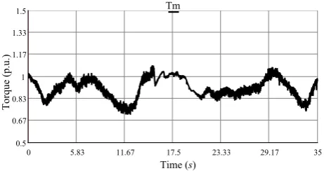
The results obtained illustrate that the system can send power in different regions of operation according to the chan-ges of wind sequence. The electrical and mechanical varia-bles can be kept within the desired values, that is, a constant value at the DC-link, a value ofPpccaccording to the wind,
Qpcckept at a low value for a unit power factor and a smooth
torque variation.
0 5.83 11.67 17.5 23.33 29.17 35
Time (s)
0.5 0.67 0.83 1 1.17 1.33 1.5
Torque (p.u.)
[image:11.595.42.284.82.364.2]Tm
Fig. 21 Mechanic torque obtained in all wind operating regions.
7.2 Load variations
In this case study, when the wind system is sending 2 MW of nominal power to the power system, an external load with a value of 1 MW is connected in the test system at 6 seconds of the simulation time. That is a 50% of the nominal value of
the wind turbine; it is removed 15 seconds later. This causes that the power system receives only 1 MW of the 2 MW generated by the wind turbine while the load is connected. Fig. 22 shows the scheme used in this case study, where the switch S1allows the insertion and removal of the load.
PMSG
3ϕ CACA
External load 1 MW
S1
2 MW
0.69 kV L-L
∆-Y
0.69 kV/230 kV
β
Vw=11.5 m/s
Wind turbine BTB Vdc=1200 Vconverter
fsw1=1988 Hz
[image:11.595.303.535.175.301.2]fsw2=4860 Hz
Fig. 22 External load connected to the test system.
Fig. 23 illustrates the behavior of the electrical variables when the load is connected. This simulation was carried-out considering a constant wind speed value ofvw=11.5 m/s
(see Fig. 23 a)). It can be observed from Fig. 23 b) that the power delivered to the grid is reduced in 50 %. Fig. 23 c) shows that the control system helps to maintain the DC-link voltage in a constant value of 1200 V, and it is not affected by the load change. The Fig. 23 d) shows that the electrical power sent by the wind turbine at the PCC is not affected when this load change occurs.
10.5 11 11.5 12 12.5
Wind speed (m/s)
Vw
500E3 1E6 1.5E6 2E6 2.5E6
Active power (W)
P source
8E2 9.17E2 1.03E3 1.15E3 1.27E3 1.38E3 1.5E3
Volta
g
e (
V
) Vdc
0 5.83333 11.66667 17.5 23.33333 29.16667 35
Time (s) -1E6
0 1E6 2E6 3E6
Electrical
power (W,VAR)
P Q
a)
b)
c)
[image:11.595.298.541.492.735.2]d)
[image:11.595.43.274.514.636.2]The obtained results for this case study show that the system is capable of return to its steady state after that a load change has been applied.
7.3 Solid three-phase to ground fault
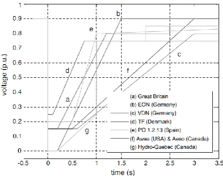
[image:12.595.298.535.199.460.2]This case study tests the Low Voltage Ride-Through (LVRT) capability, which is a requirement for a wind turbine to re-main connected to the system without tripping when a short-duration fault occurs in the power system [48, 49]. Voltage disturbances occur up to specified time periods associated with voltage levels, as described by the grid codes [50] (see Fig. 24). The line of each code indicates that the system must remain in operation if the voltage stays in the zone above the line of the code, according to the time established.
Fig. 24 LVRT requirements for different grid codes [50].
A three-phase fault is applied at the middle of the second transmission system (see Fig. 25), after 6 seconds of simu-lation time, when the system is already operating in steady state; the fault is maintained for 0.16 seconds and then re-moved. The voltages and currents at load terminals in the system are presented and analyzed. A solid three-phase fault is applied, as it involves considerable mechanical and elec-trical stresses.
β
PMSG
F 3ϕ
∆-Y CA
CA
Double circuit transmission line
Vw=11.5 m/s
Wind turbine
Tmnom=787kN-m
BTB converter
Vdc=1200 V fsw1=1988 Hz
fsw2=4860 Hz
2 MW
0.69 kV L-L
PCC
[image:12.595.44.274.311.492.2]0.69 kV/230 kV
Fig. 25 LVRT capability test system.
In Fig. 26 the behavior of voltages and currents in the presence of the fault is shown. The fault is applied at the middle of the second transmission system at 50 km. After the fault is applied, these currents reach an amplitude of 3.5 p.u., when the fault is removed they return to their pre-fault state.
0.2 0.4 0.6 0.8 1
1.2 Vpcc
0 1 2 3 4
Current in PCC
(
p.u.) Ipcc
5.8 5.92 6.03 6.15 6.27 6.38 6.5 Time (s)
0 0.25 0.5 0.75 1 1.25 1.5
Voltages in
the
fault point (p.u.)
Vfault
a)
b)
c)
V
oltage in
the
PCC
(
p.u.
)
Fig. 26 Behavior of the three-phase voltages and currents in the PCC.
Fig. 27 shows the power exchange at the inverter ter-minals during the disturbance condition; the PMSG must supply the necessary reactive power to maintain the voltage level at the PCC. This is achieved with the control scheme of the Fig. 28, in which is added a loop of control with a vpcc
reference.
Fig. 29 shows the behavior of the torque and the me-chanical speed. It can be observed that they can go back to their nominal values once the three-phase fault has been re-moved.
[image:12.595.55.278.656.730.2]0.92 0.94 0.96 0.98 1 1.02 1.04
Active power (p.u.)
Ppcc
0.05 0.1 0.15 0.2 0.25
Reactive power (p.u.)
Qpcc
5 5.83 6.67 7.5 8.33 9.17 10
Time (s)
0.8 0.9 1 1.1 1.2 1.3 1.4
DC-link v
olta
g
e (
p.u.
) Vdc
a)
b)
[image:13.595.42.282.84.350.2]c)
Fig. 27 Behavior of the power exchange in the PCC.
iqi
PI 0
-+
PI -+
vpcc*pu i
q ref vpccpu
[image:13.595.45.281.383.454.2]mq1
Fig. 28 Change of the reference foriqcurrent when a fault to ground
occurs.
5 5.83 6.67 7.5 8.33 9.17 10
Time (s) 0.95
0.99 1.03 1.08 1.12 1.16 1.2
Mechanical speed
(
p.u.
) Wpu
0 0.25 0.5 0.75 1 1.25 1.5
Mechanical torque (p.u.)
Tm
a)
b)
Fig. 29 Behavior of the mechanical variables in presence of a three-phase fault.
8 Conclusions
In this contribution a full model of a PMSG wind turbine in-cluding a BTB converter in thedqreference frame has been proposed and discussed in detail. This model was used for the development of linear control strategies for the wind sys-tem. The designed control strategies consider the operation of the variable speed wind turbine within three operating re-gions, and allow an optimal power extraction from the wind on a wide range of values, with a safe and optimal operation for the power system.
The control strategies have been implemented in Arduino due cards in order to test their behavior under transient con-ditions. Considerations about their implementation were also presented. By using the developed model and the imple-mented control strategies, real-time simulations were carried-out.
Three case studies have been presented. The first case shows that the control strategies for the converters can main-tain its operation in wide regions of wind, and make possible to extract the optimal power for each wind condition. The second case study evaluates the performance of the wind system when a change of load occurs. It can be observed that the system can go back to its pre-disturbance steady state. Finally, the last case study has shown that the system can keep constant voltage at the PCC when a three-phase fault was applied at the middle of the second transmission system; this according to the grid codes.
Acknowledgments
The authors want to acknowledge the Universidad Aut´onoma de San Luis Potos´ı (UASLP) through the Facultad de Inge-nier´ıa, the Facultad de Ingenier´ıa El´ectrica of the Univer-sidad Michoacana de San Nicol´as de Hidalgo (UMSNH), and the Institute for Energy and Environment, University of Strathclyde, for the facilities granted to carry-out this inves-tigation.
Appendix A: Parameters of the test system
[image:13.595.44.281.495.680.2]The parameters of the test system used in this research are:
Table 1 Parameters of the wind turbine.
Wind sequence parameter Value Shaft height of the wind turbineh 80 m Rated wind speedvωn 11.5 m/s
cut-in wind speedvmin 5 m/s
Table 2 PMSG parameters.
Parameters Value Units
Nominal powerPnom 2 MW
Stator resistanceRs 0.008 Ω
Leakage inductances indq-frameLd,q 0.0003 H
Leakage inductanceLls 0.00002727 H
Permanent magnet fluxλm0r 3.86 wb
Number of polesP 120
Mechanical speedωm 2.5 rad/s
Inertia constantJ 8000 kg·m2
Viscosity coefficientBm 0.00001349 N·m·s
Table 3 BTB converter and grid parameters.
Parameters Value Units
Line resistanceR1,2 0.009 Ω
Line inductance of the generator sideL1 0.0003 H
Line inductance of the grid sideL2 0.000125 H
CD-link voltagevdc 1200 V
RMS voltage of the linev1,2 690 V
Inductance of the gridLn 0.000175 H
Switching frequency atωrnom,fsw1 1988 Hz
switching frequencyfsw2 4860 Hz
Frequency index modulationmf1 81
Frequency index modulationmf2 81
Table 4 Transmission line parameters.
Parameters Value Units
Number of phases 3
Positive sequence series resistance 0.0996228 Ω/km Positive sequence series inductive reactance 0.514432 Ω/km Positive sequence shunt capacitive reactance 0.315 MΩ/km Zero sequence series resistance 0.3618376 Ω/km Zero sequence series inductive reactance 1.227747 Ω/km Zero sequence shunt capacitive reactance 0.34514 Ω/km
Length of the line 100 km
References
1. Q. Shi, G. Wang, L. Fu and L. Yuan and H. Huang.State-space averaging model of wind turbine with PMSG and its virtual inertia control. Industrial Electronics Society, IECON 2013 - 39th Annual Conference of the IEEE, Nov. 2013; 1880-1886.
2. M. Martins, A. Perdana, P. Ledesma, E. Agneholm and O. Carl-son.Validation of fixed speed wind turbine dynamic models with measured data. Renewable Energy, 2007;32(8): 1880-1886. 3. Hamid Reza Najafi and Farshad Dastyar. Dynamic maximum
available power of fixed-speed wind turbine at islanding opera-tion. International Journal of Electrical Power & Energy Systems, 2013;47: 147-156.
4. Deok-Chul Kim, Joon-Ho Choi, Won-Wook Jung, Ju-Yong Kim and II-Keun Song.Modeling and MPPT Control in DFIG-Based Variable-Speed Wind Energy Conversion Systems by Using RTDS. Journal of International Council on Electrical Engineering, 2011;
1(4): 430-436.
5. S.M. Muyeen, Ahmed Al-Durra and J. Tamura.Variable speed wind turbine generator system with current controlled voltage
source inverter. Energy Conversion and Management, 2011;
52(7): 2688-2694.
6. H. Shariatpanah, R. Fadaeinedjad and M. Rashidinejad.A New
Model for PMSG-Based Wind Turbine With Yaw Control. IEEE
Transactions on Energy Conversion, 2013;28(4): 929-937.
7. Hiskens, I.A.Dynamics of Type-3 Wind Turbine Generator Mod-els. Power Systems, IEEE Transactions on, Feb. 2012;27(1): 467-474.
8. Junfei Chen, Hongbin Wu Sun, Weinan Jiang, Liang Cai and Caiyun Guo.Modeling and simulation of directly driven wind tur-bine with permanent magnet synchronous generator. IEEE PES Innovative Smart Grid Technologies, May 2012; 1-5.
9. F. Blaabjerg, M. Liserre and K. Ma.Power Electronics Converters for Wind Turbine Systems. IEEE Transactions on Industry Appli-cations, March 2012;48(2): 708-719.
10. M. Singh, S. Surya.Dynamic models for wind turbines and wind power plants. National Renewable Energy Laboratory, 2011. 11. R. Ben Ali, H. Schulte, and A. Mami.Modeling and simulation
of a small wind turbine system based on PMSG generator. 2017 Evolving and Adaptive Intelligent Systems (EAIS), June 2017; 1-6.
12. E. M. Youness and Z. Othmane.Dynamic modeling and control of a wind turbine with MPPT control connected to the grid by using PMSG. 2017 International Conference on Advanced Technologies for Signal and Image Processing (ATSIP), Oct. 2017; 1-6. 13. G. H. Kim, Y. J. Kim, M. Park, I. K. Yu and B. M. Song.
RTDS-based real time simulations of grid-connected wind turbine gen-erator systems. 2010 Twenty-Fifth Annual IEEE Applied Power Electronics Conference and Exposition (APEC), March 2010; 2085-2090.
14. M. Yin, G. Li, M. Zhou and C. Zhao.Modeling of the Wind Tur-bine with a Permanent Magnet Synchronous Generator for Inte-gration. IEEE Power Engineering Society General Meeting, July 2007; 1-6.
15. A. B. Dehkordi, A. M. Gole and T. L. Maguire.Permanent Mag-net Synchronous Machine Model for Real-Time Simulation. Inter-national Conference on Power Systems Transients (IPST05), Jun 2005.
16. L. A. Soriano, W. Yu and J. J. Rubio.Modeling and Control of Wind Turbine. Mathematical Problems in Engineering, June 2013; Article ID 982597: 13 pages.
17. W. Liu, L. Chen, J. Ou and S. Cheng. Simulation of PMSG wind turbine system with sensor-less control technology based on model reference adaptive system. Electrical Machines and Sys-tems (ICEMS), 2011 International Conference on, Aug 2011; 1-3. 18. Jemaa Brahmi, Lotfi Krichen and Abderrazak Ouali.A compara-tive study between three sensorless control strategies for PMSG in wind energy conversion system. Applied Energy, 2009;86(9): 1565-1573.
19. Ortega, D.F., Shireen, W. and Castelli-Dezza, F.Control for grid connected PMSG Wind turbine with DC link capacitance reduc-tion. Transmission and Distribution Conference and Exposition (T D), 2012 IEEE PES, May 2012; 1-8.
20. B. Malinga.Modeling and control of a wind turbine as a dis-tributed resource. 35th Southeastern Symposium on System The-ory, March 2013; 108-112.
21. V. I. Utkin.Sliding Modes in Control and Optimization. Commu-nications and Control Engineering Series, Springer, 1992. 22. B. Beltran, T. Ahmed-Ali, M. E. H. Benbouzid and A. Haddoun.
Sliding mode power control of variable speed wind energy con-version systems. IEEE International Electric Machines and Drives Conference (IEMDC ’07), May 2007: 943-948.
23. A. S. Yilmaz and Z. zer.Pitch angle control in wind turbines above the rated wind speed by multi-layer perceptron and radial basis function neural networks. Expert Systems with Applications, Au-gust 2009;36(6): 9767-9775.
24. X. Yao, X. Su and L. Tian.Wind turbine control strategy at lower wind velocity based on neural network PID control. International Workshop on Intelligent Systems and Applications (ISA ’09), May 2009: 1-5.
25. H. H. Lee, P. Q. Dzung, L. M. Phuong, L. D. Khoa and N. H. Nhan.
doubly fed induction generator. International Forum on Strategic Technology (IFOST ’10), October 2010: 134-139.
26. Y. S. Qudaih, M. Bernard, Y. Mitani and T. H. Mohamed.Model predictive based load frequency control design in the presence of DFIG wind turbine. 2nd International Conference on Electric Power and Energy Conversion Systems (EPECS ’11), November 2011: 1-5.
27. Chang Kang, Xue Feng, Fang Yongjie and Yu Yuehai. Com-parative simulation of dynamic characteristics of Wind Turbine
Doubly-Fed Induction Generator based on RTDS and MATLAB.
Power System Technology (POWERCON), 2010 International Conference on, Oct 2010; 1-8.
28. M. Tursini, L. Di Leonardo, C. Olivieri and E. D. Loggia.Rapid Control Prototyping of IPM Drives by Real Time Simulation. 2013 8th EUROSIM Congress on Modelling and Simulation, Sept 2013; 364-371.
29. T. Yao, I. Leonard, R. Ayyanar and M. Steurer.Single-phase three-stage SST modeling using RTDS for controller hardware-in-the-loop application. 2015 IEEE Energy Conversion Congress and Exposition (ECCE), Sept 2015; 2302-2309.
30. R. Pe˜na and A. Medina.Real time simulation of a power system including renewable energy sourcesNorth American Power Sym-posium (NAPS), Sept 2012; 1-5.
31. Ming Yin, Gengyin Li, Ming Zhou and Chengyong Zhao. Model-ing of the Wind Turbine with a Permanent Magnet Synchronous Generator for Integration. Power Engineering Society General Meeting. IEEE, Jun 2007; 1-6.
32. Robert J. Howlett, Nacer Kouider M’Sirdi, Aziz Naamane, Ali Sayigh, Y. Errami, M. Ouassaid and M. Maaroufi.Control of a PMSG based Wind Energy Generation System for Power Maxi-mization and Grid Fault Conditions. Mediterranean Green Energy Forum 2013: Proceedings of an International Conference MGEF-13, Energy Procedia, 2013;42: 220-229.
33. T. Ackermann.Wind Power in Power Systems. Wiley,2005. 34. Gonz´alez-Longatt, FM., Amaya, O., Cooz, M., Duran, L., Peraza,
C., Arteaga, FJ. and Villanueva C.Modelaci´on y simulaci´on de la velocidad de viento por medio de una formulaci´on estoc´astica. Revista INGENIER´IA UC, Dec 2007;14(3): 7-15.
35. Wai, R.-J., Lin, C.Y. and Chang, Y.R. Novel maximum-power-extraction algorithm for PMSG wind generation system. Electric Power Applications, IET, March 20071(2): 275-283.
36. Quincy Wang and Liuchen Chang.An intelligent maximum power extraction algorithm for inverter-based variable speed wind tur-bine systems. Power Electronics, IEEE Transactions on, Sept 2004;19(5): 1242-1249.
37. Siegfried Heier.Grid Integration of Wind Energy Conversion Sys-tems. Wiley, 1998.
38. Krause, P.C. and Wasynczuk, O. and Sudhoff, S.D. and Pekarek, S.Analysis of Electric Machinery and Drive Systems. IEEE Press Series on Power Engineering, 2013.
39. Rafael Pe˜na, Aurelio Medina and Olimpo Anaya-Lara. Steady-state Solution of Fixed-speed Wind Turbines Following Fault Con-ditions Through Extrapolation to the Limit Cycle. IETE Journal of Research, Jan 2011;57(1): 12-19.
40. Alcala, J., Cardenas, V., Ramirez-Lopez, A.R. and Gudino-Lau, J.Study of the bidirectional power flow in Back - to - Back con-verters by using linear and nonlinear control strategies. Energy Conversion Congress and Exposition (ECCE), 2011 IEEE, Sept 2011; 806-813.
41. J. Segundo and A. Medina.Modeling of FACTS Devices Based on SPWM VSCs. IEEE Transactions on Power Delivery, Oct 2009;
24(4): 1815-1823.
42. Bianchi, F.D., De Battista, H. and Mantz, R.J.Wind Turbine Con-trol Systems, principles, modelling and gain scheduling design. Advances in Industrial Control series, Springer, 2007.
43. A. Tob´ıas, R. Pe˜na, J. Morales and G. Gutierrez.Modeling of a wind turbine with a permanent magnet synchronous generator for
real time simulations. 2015 IEEE International Autumn Meeting on Power, Electronics and Computing (ROPEC), Nov 2015; 1-6. 44. Van der Broeck, H.W., Skudelny, H.-C. and Stanke, G.V.Analysis
and realization of a pulsewidth modulator based on voltage space vectors. Industry Applications, IEEE Transactions on, Jan 1988;
24(1): 142-150.
45. RTDS technologies. Real Time Digital Simulator Tutorial Manual. Winnipeg Canad´a 2015.
46. Dommel, H.W. Digital Computer Solution of Electromagnetic Transients in Single-and Multiphase Networks. Power Apparatus and Systems, IEEE Transactions on, Apr 1969;88(4): 388-399. 47. Phillips, C.L. and Nagle, H.T.Digital control system analysis and
design. Prentice-Hall, 1984.
48. H. Ali Mohd.Wind energy systems, solutions for power quality and stabilization. CRC Press, 2012.
49. V. Pagola, R. Pe˜na and J. Segundo.Low voltage ride-through anal-ysis in real time of a PV-Wind hybrid system. 2015 IEEE Inter-national Autumn Meeting on Power, Electronics and Computing (ROPEC), Nov 2015; 1-6.
50. Abad, G., L´opez, J., Rodr´ıguez, M., Marroyo, L. and Iwanski, G.

![Fig. 5 Diagram of the PMSG wind turbine control [43].](https://thumb-us.123doks.com/thumbv2/123dok_us/1420610.94799/5.595.300.522.288.437/fig-diagram-pmsg-wind-turbine-control.webp)