Efficient parameter identification and model selection in nonlinear dynamical systems via sparse Bayesian learning

http://eprints.whiterose.ac.uk/152298/

Version: Published Version

Proceedings Paper:

Fuentes, R., Dervilis, N. orcid.org/0000-0002-5712-7323, Worden, K.

orcid.org/0000-0002-1035-238X et al. (1 more author) (2019) Efficient parameter

identification and model selection in nonlinear dynamical systems via sparse Bayesian

learning. In: Journal of Physics: Conference Series. 13th International Conference on

Recent Advances in Structural Dynamics (RASD), 15-17 Apr 2019, Valpre, Lyon, France.

IOP Publishing .

https://doi.org/10.1088/1742-6596/1264/1/012050

[email protected] https://eprints.whiterose.ac.uk/

Reuse

This article is distributed under the terms of the Creative Commons Attribution (CC BY) licence. This licence allows you to distribute, remix, tweak, and build upon the work, even commercially, as long as you credit the authors for the original work. More information and the full terms of the licence here:

https://creativecommons.org/licenses/

Takedown

If you consider content in White Rose Research Online to be in breach of UK law, please notify us by

PAPER • OPEN ACCESS

Efficient parameter identification and model selection in nonlinear

dynamical systems via sparse Bayesian learning

To cite this article: R. Fuentes et al 2019 J. Phys.: Conf. Ser. 1264 012050

Content from this work may be used under the terms of theCreative Commons Attribution 3.0 licence. Any further distribution of this work must maintain attribution to the author(s) and the title of the work, journal citation and DOI.

Published under licence by IOP Publishing Ltd 1

Efficient parameter identification and model selection

in nonlinear dynamical systems via sparse Bayesian

learning

R. Fuentes, N. Dervilis, K. Worden, E.J. Cross

Dynamics Research Group, Department of Mechanical Engineering, University of Sheffield, Mappin Street, Sheffield, S1 3JD, UK

E-mail: [email protected]

Abstract.

Bayesian inference plays a central role in many of today’s system identification algorithms. However, one of its major drawbacks is that it often requires solutions to analytically intractable integrals, and this has led to solutions via Markov Chain Monte Carlo (MCMC). Today, few Bayesian system identification methods can compete with the robustness of the family of MCMC solutions. However, MCMC suffers severely from its computational cost.

Partly fuelled by the field of Compressive Sensing (CS), an interest in the machine learning community has arisen in sparse linear regression. Its value in identification of dynamical systems has also recently started to receive some attention. The idea is to represent the range of possible candidate functional forms that have generated a specific data set using a dictionary, and to then apply standard Lasso regression to select the “best” basis, with sparsity constraints. A major problem in this approach is that Lasso regression (and its derivatives) requires tuning of the regularisation parameter. In this paper, a procedure for selecting the “best basis” (and thus performing both model selection and system identification) is presented through a sparse Bayesian learning approach. Sparsity is induced via a hierarchical Gaussian prior and an approximation to the posterior distribution is sought using an iterative optimisation scheme for finding the optimal hyper-priors that govern prior and hence, the level of sparsity in the solution. The method is applied to five systems of engineering interest, which include a baseline linear system, an additive quadratic damping term, cubic stiffness (Duffing oscillator), Coulomb damping and a Bouc-Wen hysteresis model. The results are shown using numerical simulations. It is shown that this approach can identify not only the correct model parameters, but whether a nonlinearity is present in the system as well its type. With the formulation being Bayesian, it also yields estimates of uncertainty over the selected basis functions and predicted responses.

1. Introduction

The task of identifying and estimating nonlinearities in dynamical systems is an important task of engineering and scientific interest, and one particularly relevant to structural dynamics. A general Single Degree-of-Freedom (SDOF) nonlinear harmonic oscillator can be characterised by the well known equation of motion,

my¨+cy˙+ky+g(y,y˙) = 0 (1)

g(y,y˙). In general, identification of the parameters of the linear system can be achieved in a straightforward way by means of least-squares estimation. This has been thoroughly explored in the system identification literature, and in the case of structural dynamics has been generalised to multiple degrees-of-freedom and forms the basis of experimental modal analysis. Estimation of parameters becomes more difficult when the nonlinear term begins to play a non-negligible role. Examples of this are numerous across structural dynamics and other scientific domains. Geometric nonlinearities, for example, can introduce cubic displacement terms by settingg(y) =k2y

3

. This leads to the well-known Duffing oscillator, which is classically studied in the nonlinear system identification literature. Friction and hysterisis also introduce nonlinearities in a wide range of different forms; a good example of this is the Coulomb friction model which sets g( ˙y) = sgn( ˙y). The form of the nonlinearity could be completely different as is the case, for example, in a pendulum whereg(y) = sin(y) (withy in polar coordinates).

Estimating the parameters of any one class of nonlinear system is clearly an important and useful task and one which poses a difficult problem. However, in a realistic identification task one may not even be sure of the exact form ofg( ˙y, y) and so, as discussed in [1], one must start by first identifying whether a nonlinearity is present in the first place, identifying the type of nonlinearity and then estimating the associated parameters.

This paper proposes a technique based on sparse Bayesian learning [2] that is able to simultaneously solve this combined parameter identification and model selection task. Before describing the particular approach proposed here, it is worth discussing some of the methods already existing for this task, and reviewing the state-of-the-art in the topic. No attempt is made in this paper at reviewing the vast literature of nonlinear system identification. The reader is instead referred to some excellent recent reviews and tutorials for this [1].

The key question being investigated in this paper is that of how to accurately recover the correct equations of motion of a dynamical system together with the associated parameters. Individually, both of these tasks have received a significant amount of attention, both within the remit of structural dynamics as well as in the more general context of dynamical systems. However, combined model selection and parameter estimation is a significantly more challenging task. Models of higher complexity tend to also be better predictors and successful model comparison requires one to take this into account and balance complexity against quality of fit. Bayesian inference has emerged as a powerful tool to address exactly this type of problem; it has been studied in the field of system identification owing to its ability to quantify uncertainty in parameter estimates [3, 4]. This uncertainty quantification leads directly to the idea of Bayesian model comparison [5, 6], where one seeks to compare the quality of fit of different models according to posterior probability distributions (after observing evidence) over them.

Bayesian inference, applied to the parameter estimation problem, takes the usual form,

p(θ|Y) = p(Y|θ)p(θ)

p(Y) (2)

whereθare the unknown parameters to be estimated andYis the set of (multivariate) observed data. There are three probabilities on the right-hand side of Equation (2): the prior, the likelihood and the marginal. The prior, p(θ), should represent a prior belief about the process before it is observed. The likelihood,p(Y|θ), represents the distribution of the model error, with respect to the parameters. The marginal, p(Y), is often an intractable integral, with no closed form solution available. There are various flavours for approximate and numerical solutions to the Bayesian inference problem, although these will not be discussed at length here.

3

have fewer parameters than a complex nonlinear hysteretic model. The issue of dimensionality in MCMC schemes was identified early-on in [7] and the reversible-jump MCMC was devised as an algorithm for sampling across spaces of different dimensions, with appropriate dimensionality balancing laws. While this has been applied in the context of system identification in structural dynamics [8], RJ-MCMC is cumbersome, difficult to implement and computationally intensive. An alternative has been suggested that makes use of Sequential Monte Carlo (SMC) and Approximate Bayesian Computation (ABC) in the context of structural dynamics [9] and in biological systems modelling [10]. The ABC approach enjoys the benefit of being able to jump between different model spaces without having to define a mapping between the different dimensions, as in RJ-MCMC. In addition, using SMC allows for a flexible choice of prior functional forms and so avoids the restrictiveness of the Gaussian assumption, which may or may not be applicable to the problem at hand.

One common drawback of the sampling-based approaches is their computational burden. Moreover, a challenge in the general Bayesian model comparison framework is that one has to specify a-priori the exact model forms to be compared. This may be a hinderous if one is trying to identify the type of nonlinearity, or simply whether a nonlinearity exists amongst a vast number of possible model forms. Note that a nested sampling approach to ABC inference has been investigated in [11], which addresses its computational burden.

This paper explores a rather different approach to combined parameter estimation and model selection. The problem is posed as a large parameter estimation task where each parameter, in effect, represents a different model form. The idea is borrowed from the emerging field of Compressive Sensing (CS), which provides a basis for inferring signals when sampled under the traditional Nyquist sample rate [12]. In CS, signals are represented by a large over-complete dictionary D, where the columns ofDcontain candidate vectors that could form a basis for the signal x,

x=Dβ (3)

where β is a vector of weights that one would like to solve for to estimate x from D. As it is, Equation (3) could be solved without complication via a least-squares procedure. However, CS introduces the idea of sub-sampling x by means of a random transformation applied to both x and D. This turns the problem into a massively ill-posed linear regression problem; there are too many columns for the number of available rows. The key to all of this is in the solution of this badly-posed linear estimator, which is achieved by using an L1 regularised linear regression called the Least absolute shrinkage and selector operator (Lasso) [13]. The regularisation introduced by the Lasso approach allows for a solution of the over-determined problem, under the assumption that x is sparse in the domain of D. That is, the signal of interest can be accurately represented using only a few of the candidate vectors present in D. It is an intuitive idea that has revolutionised the field of signal processing.

The idea of this paper is to view the combined parameter estimation and model selection problem as one of sparse regression. To see how this can be applied to dynamical systems, the formulation of a dynamical system in its state-space form is considered, where one is interested in estimating the functional form of mapping between the state vector xand its first derivative

˙x

˙

x=f(x) +ε (4)

where f(x) defines the dynamics of the system andε is an additive noise term, which is to be modelled as Gaussian with zero mean and variance σ2

. The idea here is to define f(x) to be a sum of possible candidate function evaluations of the state vector, encoded in a dictionary D, so that,

˙

where each column in D(x) defines a candidate model form. For example, D(x) could include constant offset, linear and polynomial terms as well as trigonometric and discontinuous functions,

D={1,x,x2,x3, ...,sin(x),cos(x),sign(x), ...} (6)

Note thatD(x) is a function of the state vector because the candidate functional forms it defines are evaluated numerically on the state vector. In the structural dynamics case, this could be, but is not restricted to, a two-dimensional displacement and velocity vector.

This problem formulation requires the use of a sparse solver, in order to select only the columns of D1

that are relevant with respect to the observed state. It is at this point that the use of sparse Bayesian learning [2] becomes relevant, as it is designed to solve exactly this type of ill-posed linear estimator. The focus on Bayesian learning with sparsity constraints is the key contribution of this paper.

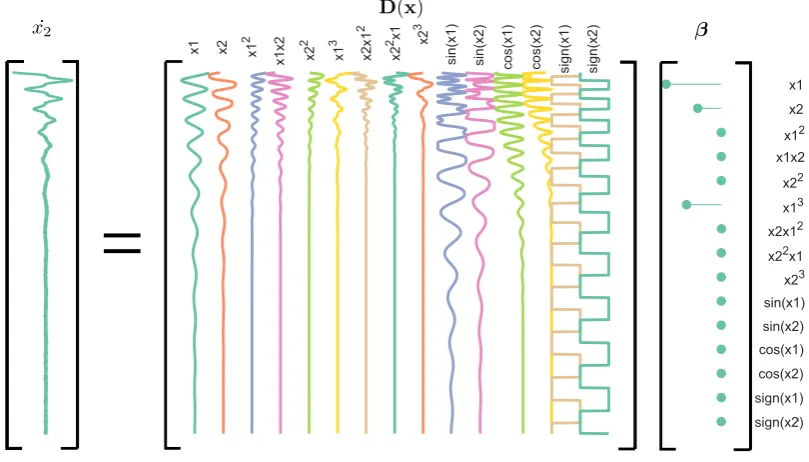
This idea is illustrated in Figure 1, which shows the solution to Equation (5) using sparse Bayesian learning (discussed in Section 2). The illustration uses the free-decay response of a Duffing oscillator and the different candidate terms that formD(x) are shown together with the sparse solution to β, which in this case yields non-zero coefficients on all terms except for x1,

x2 and x31 (where x1 is displacement andx2 is velocity).

In [14], a similar problem formulation is presented in terms of evaluating different candidate functional forms in a state-space and using a combination of symbolic regression and genetic programming to find the symbolic forms that best match an observed time series, while following conservation laws. While the general idea is laid out, the approach to optimisation lacks a natural balance between complexity and predictive accuracy. A genetic program might not naturally prefer solutions that are simple, or parsimonious. Sparsity is clearly a useful tool in solving Equation (5) with a parsimonious representation. The use of sparse linear regression (Lasso) to solve this type of problem has been investigated in [15] which deals with the general problem of recovering the governing physical laws from observed data. This is a step in the right direction, but the use of the Lasso implies the use of a tuning parameter that completely dictates the level of sparsity in the solution and hence the complexity and predictive ability of the solver. This paper builds on some of the ideas of [14] and [15] in terms of the problem formulation, but deviates in the solution to the problem. The authors are particularly interested in the investigation of Bayesian learning algorithms for the problem and this forms the focus of the current paper.

Section2will outline the key elements of the theory behind sparse Bayesian computation and will put an emphasis on comparing this approach with the non-probabilistic methods. Section

3 presents a series of numerical experiments on several systems that are of interest to nonlinear dynamics: a single degree-of-freedom system with quadratic and cubic nonlinearities, Coulomb friction and a Bouc-Wen hysteretic system. Section 4 provides a critical discussion of these results focusing on the practical limitations on the use of this algorithm. Finally, Section 5

summarises the conclusions of the paper.

2. Sparse Bayesian learning

Sparse learning is used here to provide a solution to the problem of Equation (5) that switches off any columns ofDthat do not significantly contribute to the observed dynamics. The classical solution to learning in sparse linear models is the Lasso [13]. One of the major limitations of the Lasso is that it does not give a definite answer to the appropriate level of sparsity that represents the signal. This is due to its non-probabilistic formulation. In this paper, sparse Bayesian learning is used in order to derive posterior probability distributions over the model weightsβand the predictive outputsx, whilst enforcing sparse solutions. The particular flavour of Bayesian inference that will be used here is the Relevance Vector Machine (RVM) [2].

5

˙ x₂

D(x)

β

Figure 1. Illustration of the problem formulation on a free decaying Duffing oscillator. The second state derivative (acceleration) is given in terms of candidate polynomial, trigonometric and discontinuous functions ofx, and a sparse Bayesian solution toβis shown, indicating which terms of the dictionary are active (non-zero).

2.0.1. Formulation of the RVM The presentation of the RVM in this paper essentially follows that of Tipping [2]. The RVM solves the following regression model,

y=

N

i=1

di(x)βi. (7)

The reader will recognise this as a standard regression model, where as before, the weight vector is represented by β= [β1, ..., β_N]. The basis function set is represented by D(x) = [d1, ...,d_N]. The RVM is designed to only select a sufficient and appropriate number of relevant vectors in D(x) that explain the observed data well, using sparsity constraints.

The observations of the model are assumed to be corrupted with noise, and this is modelled by a target vector,t,

t=y+ε (8)

where εis the noise term andy is the representation of the signal, as defined by Equation (7). The key ingredient in the formulation of the RVM is the form of the prior distribution of the parameter vector, p(β|α), (whereα is ahyperparameter) as it is the form of this prior that enforces sparsity. More specifically, this is given as a hierarchical Gaussian distribution, which is a conjugate prior to a Gaussian distribution and thus yields algebraic forms that are tractable. The form of this hierarchical prior is,

p(β|α) =

M

i=1

N(βi|0, α−

1

i ). (9)

hierarchical nature of this prior arises from the fact that prior distribution over this prior needs to be defined. This includes both the variance terms for the prior,α, as well as the signal noise variance σ2

. Instead of setting a prior over the variance directly, a prior is set over its inverse

ρ=σ−2:

p(α) =

M

i=1

Γ(a)−1baαa−1e−bα (10)

p(ρ) = Γ(c)−1

dcαc−1e−dρ (11)

where Γ is the Gamma function and a, b and c, d are hyperparameters of the prior and noise variance respectively (in effect, “hyper-hyperparameters”). In effect, it is these parameters that control whether the prior is sparse or not, and in practice they need to be set such that p(β|α) becomes infinitely peaked around zero, to within numerical precision. For a more detailed description of the role of these hierarchical hyper-priors see [2]. Assuming a Gaussian likelihood function, the posterior distribution over the parameters can be written using Bayes’ theorem as,

p(β|t,α, σ2) = p(t|β, σ 2

)p(β|α)

p(t|α, σ2₎ . (12)

Using standard Gaussian identities, this yields a Gaussian distribution,

p(β|t,α, σ2) =N(µ,Σ) (13)

where the mean and variance are given by,

Σ= (A+σ−2D⊤D)−1

(14)

µ=σ−2ΣD⊤t (15)

Ais a diagonal matrix with the elements ofαalong its diagonal. Equations (15) and (14) define the mean and covariance of the coefficient vector β.

In order to make predictions with this model, one would wish to evaluate the distribution

p(t⋆|t,α, σ2) (wheret⋆ is a set of testing data points), which can be shown to be a multivariate

Gaussian with mean and covariance [2],

y⋆ =Dµ (16)

V⋆ =σ

2

+D⊤ΣD (17)

The predictive variance in Equation (17) is the sum of two terms: the signal noise, σ2 and the predictive uncertainty, arising from the term D⊤_ΣD.

For sparse Bayesian learning to be effectively realised one has to optimise the hyperparameter vector α that encodes the sparsity level and σ2

7 3. Numerical Experiments

In order to investigate the proposed approach to combined model selection and parameter estimation, several numerical experiments are carried out. The system being investigated here is the single degree-of-freedom oscillator of Equation (1) which contains a general nonlinearity

g( ˙y, y). The state-space formulation of the system will be used throughout this discussion, where the first element is the displacement and the second is the velocity

x1 =y (18)

x2 = ˙y (19)

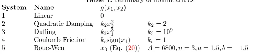
Different forms of the nonlinearityg(x1, x2) yield various systems of engineering interest. Five different cases are investigated here, summarised in Table3. The linear case, although simple is included as establishing whether the proposed algorithm is capable of ruling out the existence of any nonlinearities in the dynamic response is of fundamental interest.

The second system includes a quadratic damping term. This is representative of systems that operate in fluids and gases, where the force due to drag is non-negligible and contributes significantly towards the damping of the system. The third system is a Duffing oscillator, which arises from a cubic nonlinearity on the displacement of the system, g(x1) =k3x

3

1. The Duffing oscillator has been the subject of a large number of studies in system identification. This is both due to the complex behaviours it can generate but also because it is representative of geometric nonlinearities found in real world systems, such as that of simply-supported or cantilever beams undergoing large displacements. The fourth system is one with a Coulomb friction nonlinearity. The Coulomb model assumes that frictional force is constant (proportional to the normal load) and is only dependent on the direction of the velocity. This results in a nonlinearity of type

g(x2) = kcsign(x2) (where sign denotes the signum operator). This type of system has been of general interest in nonlinear system identification [18, 19,1] as it represents a wide range of practical structures where dry sliding occurs, such as systems with bolted joints, for example.

The fifth and last system investigated here is the Bouc-Wen model of hysteresis [20], which models a hysteretic nonlinear restoring force through a third state variable, g(x2) = x3. The dynamics of the restoring force are then described by the following nonlinear first-order differential equation,

˙

x3=

−a|x2|xn3 −bx2|xn3|+Ax2 fornodd

−a|x2|xn− 1

3 |x3| −bx2|xn3|+Ax2 forneven

(20)

Table 1. Summary of nonlinearities System Name g(x1, x2)

1 Linear 0

2 Quadratic Damping k2x 2

2 k2= 2

3 Duffing k3x31 k3= 109

4 Coulomb Friction kcsign(x1) kc= 1

5 Bouc-Wen x3 (Eq. (20)) A= 6800, n= 3, a= 1.5, b=−1.5

Each of the systems was simulated using a 4th_{-order Runge-Kutta numerical integration}

scheme, with a sample rate of 32768Hz. Note that this sample rate is significantly higher than the natural frequency of the linear system. The reason for this is to minimise the error in numerical differentiation and to minimise the introduction of artifacts of the numerical integration, which can confuse the sparse Bayesian learner. The systems with the form of their nonlinearities and the associated parameters used for the simulations are summarised in Table 3. The parameters used for the underlying linear model were m = 1, k = 1×104

and c = 20, which places the natural frequency of the underlying linear oscillator at 15.9Hz. Each of the nonlinear systems were simulated with the same parameters governing the linear model, and only varied in the additional nonlinear termg(x1, x2). The state vector,x, collected from the simulations consisted of displacement and velocity. Its derivative, ˙x, was obtained by numerical differentiation with respect to time. Of course in reality, the actual observed variables may differ from those used these case studies. However, this does not impede the application of the procedure proposed here, as long as the state variables can be computed to within reasonable accuracy by numerical differentiation/integration schemes.

A solution to the problem outlined in Equation (5) is then sought, in terms of a sparse coefficient vector β that links the state x to its derivative ˙x through selection of appropriate columns of D(x). The definition of the dictionary is critical to the success of this algorithm. For this procedure to work at all, the functional form of differential equation that describes the dynamics must be present inD. This includes any linear and nonlinear terms. In this paper, a dictionary was assembled using candidate functions that include polynomial expansion terms as well as trigonometric functions that could potentially describe the systems being studied here. The terms were as follows,

D(x) ={F(t), P1(x), ..., Pn(x),sin(x),cos(x),tan(x),sgn(x)} (21)

where Pn(x) denotes the polynomial expansion of ordern of the sum of the p state vectors (x1 +x2+...x_p)n. In this paper, polynomial orders of up to n = 6 were used as candidate functions. Furthermore, the state vector was augmented with|x|, in order to also generate the cross-terms necessary to capture the dynamics of the Bouc-Wen hysteresis of Equation (20). Note that the dictionary also includes the forcing term F(t) in the first column in order to capture the input force contribution as part of the sparse learning process. Performing this combined model-selection and parameter estimation in the case with unknown forcing would become much harder as one would have to discern whether forcing terms that are a residual of the underlying linear system are due to an internal nonlinear force or due to external forcing. The problem could be further exacerbated if the external forcing is itself generated by a nonlinear dynamical system, as is the case for example in fluid-structure interaction problems [27]. This is not treated in this paper, and instead the focus is first placed on simple forced systems with known excitation.

9

force ˙x3 for system five (Bouc-Wen). Note that in all cases, the solution to the first state derivative is trivial, since by definition ˙x1 = x2. However, it is important to note that in all cases, sparse Bayesian inference does select the linear term onx2 as the single non-zero relevant vector explaining ˙x1. These results are not shown here.

Appropriate scaling of the observed dataxis important for the success of this procedure, so all values of columns of x and ˙x have been scaled to unit standard deviation. This is critical for numerical stability, in particular when dictionary terms involve high polynomial orders or trigonometric terms such as tan(x). Furthermore, all the resulting columns of D(x) have been normalised to unit l2 norm.

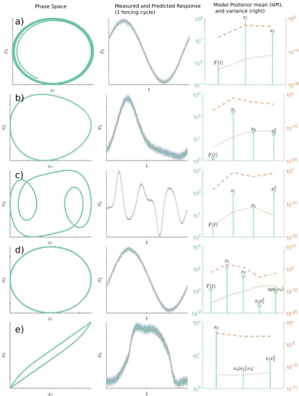
The results are presented in Figure 2 for systems one to five excited with a single sine wave of 10Hz at an amplitude of 100N. The output data were corrupted with white Gaussian noise with a variance of 0.4%, relative to the standard deviation of the observations. Note that this noise propagates through the numerical differentiation and leads to a higher variance in ˙x. The first column in Figure 2 shows the phase-space representation in terms of x1 and

x2. The second column shows the measured and predicted responses in the time domain (for one excitation cycle), where the shaded area illustrates the predictive uncertainty through the 3σ confidence interval. The third column shows the coefficient vector β resulting from sparse Bayesian inference. For clarity, only coefficients that yielded non-zero values are shown. Also, the absolute values of the coefficients are plotted so as to enable visualisation in the logarithmic domain. The posterior variances and optimised prior variance hyperparameters are shown alongside the coefficient, on the right axis. The posterior variance quantifies the posterior uncertainty around each coefficient vector. The optimised hyper-prior variance, αi for each

term is also called a “sparsity factor” as this quantifies the degree to which any given column in the dictionary contributes to sparsifying the solution. If α is low, this means that the prior assumption is that the solution will be concentrated tightly around that vector and thus deeming it “relevant”. If αis high, this implies that the vector does not contribute to a sparse solution. Terms that form a likely solution are those that have a low variance in both the posterior and the optimised hyper-prior. These tools are helpful because in practice, the RVM, or any other sparse learner may yield more non-zero terms than are true for the underlying system. However, these two variances, which result from the Bayesian treatment of the sparse solution, provide one with tools to assess how likely it is that suspected “spurious” terms are truly part of the dynamics, or have crept in from elsewhere (such as analogue or digital filtering).

rates, this effect is mitigated, and at lower sample rates more spurious terms tend to appear. Figure 2e shows the results of the Bouc-Wen hysteresis model, System 5. Note that combinations from the expansion (x1 +x2 +x3 +|x1|+|x2|+|x3|)n were used to build the candidate vectors in the dictionary (these absolute terms were present in D but not identified in other systems). In this case, the assumption is that the restoring force variable is measured. The solution to ˙x3, which contains the nonlinearity, is shown in Figure 2e for n = 2. The sparse Bayesian learner correctly identifies the terms for this model form, and its predictive performance reflects this.

4. Discussion

The results of performing combined model selection and parameter identification with sparse Bayesian learning are encouraging. The fact that the algorithm is able to identify individual terms of known difficult dynamical systems is a positive result. It is important to note that this investigation has been basic in some respects. The first is that no results are shown here for different types of forcing, something which will clearly have an influence on the identified system. The cases of random forcing, free vibration, chirp excitations and random phase multi-sines all produce some interesting results, but this falls outside the scope and length of this paper. Here, the basic concept has been laid out instead, with some simple demonstrations.

While the results that have been presented show the procedure working almost at its best, it is important to highlight that the outcome depends strongly on the simulation settings, data pre-processing and noise levels. This is an interesting point to highlight. The fact that the algorithm is sensitive to the simulation parameters makes sense given that the simulation is a dynamical system itself. Clearly the procedure needs to be validated on experimental data, but the results of the simulation raise some interesting question. For example, any amount of digital filtering of the displacements, velocities or accelerations tended to generate a solution with significantly more polynomial terms than those of the system. This makes sense, given that most pre-processing tasks could be described as passing the signals through another dynamical system, it should be no surprise that this will be identified upstream. This may also be the case for experimental data, as it will inevitably have to be pre-processed by hardware filters. However, that remains to be seen. Another factor that significantly influences the outcome of the identification in this case is the scheme for numerical differentiation required to estimate ˙x. Tools are available to perform complex interpolation schemes, but it was found that these would also have an effect on the identified system. In the end, a simple point-difference yielded the most consistent and robust results.

A final remark is that a move to multiple degrees of freedom would be straight-forward in principle under this scheme, but this is also outside the scope of this paper.

5. Conclusions

This paper has presented an approach for combined parameter estimation and model selection in nonlinear systems using sparse Bayesian learning techniques. The system identification problem has been formulated in terms of the solution to a first order differential equation that uses a dictionary containing a large number of candidate functional forms that could form part of the solution. The solution to the sparse Bayesian learning problem leverages the use of the Relevance Vector Machine (RVM) due to its computational tractability and fast implementations.

11

6. Acknowledgements

This work has been funded by the UK Engineering and Physical Sciences Research Council (EPSRC), through the Autonomous Inspection in Manufacturing and Re-manufacturing (AIMaReM) grant EP/N018427/1. Support for K. Worden from the EPSRC through grant reference number EP/J016942/1 and for E.J. Cross through grant number EP/S001565/1 is also acknowledged. The authors would also like to thank Dr. Kartik Chandrasekhar, from the Dynamics Research Group at Sheffield, for useful discussions that led to a better paper.

References

[1] Kerschen G, Worden K, Vakakis A F and Golinval J CMechanical Systems and Signal Processing 505–592 ISSN 0888-3270

[2] Tipping MJournal of Machine Learning Research 211–244 ISSN 1532-4435 [3] Beck J LStructural Control and Health Monitoring825–847 ISSN 15452255

[4] Worden K and Hensman JMechanical Systems and Signal Processing 153–169 ISSN 0888-3270

[5] MacKay D J C 2005Information Theory, Inference and Learning Algorithms(Cambridge University Press) ISBN 0521642981 (Preprint arXiv:1011.1669v3)

[6] Gelman A, Carlin J B, Stern H S, Dunson D B, Vehtari A and Rubin D B 2014 Bayesian Data Analysis, Third EditionISBN 978-1-4398-9820-8 (Preprint arXiv:1011.1669v3)

[7] Green P J and Hastie D I 2009Bioinformatics ISSN 13674811

[8] Tiboaca D, Green P L, Barthorpe R J and Worden K (Springer, Cham) pp 277–284

[9] Ben Abdessalem A, Dervilis N, Wagg D and Worden KMechanical Systems and Signal Processing 306–325 ISSN 0888-3270

[10] Liepe J, Kirk P, Filippi S, Toni T, Barnes C P and Stumpf M P HNature Protocols439–456 ISSN 1754-2189 [11] Ben Abdessalem A23`eme Congr`es Fran¸cais de M´ecanique (Association francaise de mecanique) ISSN

2491-715X

[12] Cand`es EProceedings of the International Congress of Mathematicians Madrid, August 2230, 2006 (Zuerich, Switzerland: European Mathematical Society Publishing House) pp 1433–1452 ISBN 978-3-03719-022-7 [13] Tibshirani R Regression Selection and Shrinkage via the Lasso (Preprint 11/73273)

[14] Schmidt M and Lipson HScience 81–85 ISSN 0036-8075

[15] Brunton S L, Proctor J L and Kutz J NProceedings of the National Academy of Sciences of the United States of America3932–7 ISSN 1091-6490

[16] Dempster A, Laird N and Rubin D BJournal of the Royal Statistical Society Series B Methodological 1–38 ISSN 00359246 (Preprint 0710.5696v2)

[17] Tipping M E and Faul A CProceedings of the ninth . . . 1–13 ISSN 0717-6163 (PreprintarXiv:1011.1669v3₎

[18] Dahl P RAIAA Journal1675–1682 ISSN 0001-1452

[19] Liang J W and Feeny B FNonlinear Dynamics 337–347 ISSN 0924090X

[20] Wen Y K 1976Journal of the Engineering Mechanics Division 102pp. 249–263 ISSN 0044-7951 (Preprint arXiv:1011.1669v3)

[21] Ismail M, Ikhouane F and Rodellar J Archives of Computational Methods in Engineering 161–188 ISSN 1134-3060

[22] Zhu X and Lu XProcedia Engineering 318–324 ISSN 1877-7058

[23] Charalampakis A and Koumousis VJournal of Sound and Vibration 571–585 ISSN 0022-460X [24] Charalampakis A and Dimou CComputers & Structures1197–1205 ISSN 0045-7949

[25] Spiridonakos M and Chatzi EComputers & Structures 99–113 ISSN 0045-7949

[26] Chandrasekhar K, Rongong J and Cross EMechanical Systems and Signal Processing 13–29 ISSN 0888-3270 [27] Rogers T J, Worden K, Manson G, Tygesen U and Cross E J 2018 International Conference on Noise and