Model selection and parameter estimation of dynamical systems using a novel variant of approximate Bayesian computation

This is a repository copy of

Model selection and parameter estimation of dynamical

systems using a novel variant of approximate Bayesian computation

.

White Rose Research Online URL for this paper:

http://eprints.whiterose.ac.uk/140389/

Version: Published Version

Article:

Abdessalem, A.B., Dervilis, N. orcid.org/0000-0002-5712-7323, Wagg, D. et al. (1 more

author) (2019) Model selection and parameter estimation of dynamical systems using a

novel variant of approximate Bayesian computation. Mechanical Systems and Signal

Processing, 122. pp. 364-386. ISSN 0888-3270

https://doi.org/10.1016/j.ymssp.2018.12.048

[email protected]

https://eprints.whiterose.ac.uk/

Reuse

This article is distributed under the terms of the Creative Commons Attribution-NonCommercial-NoDerivs

(CC BY-NC-ND) licence. This licence only allows you to download this work and share it with others as long

as you credit the authors, but you can’t change the article in any way or use it commercially. More

information and the full terms of the licence here: https://creativecommons.org/licenses/

Takedown

If you consider content in White Rose Research Online to be in breach of UK law, please notify us by

Model selection and parameter estimation of dynamical

systems using a novel variant of approximate Bayesian

computation

A. Ben Abdessalem

⇑

_{, N. Dervilis, D. Wagg, K. Worden}

Dynamics Research Group, Department of Mechanical Engineering, University of Sheffield, Mappin Street, Sheffield S1 3JD, United Kingdom

a r t i c l e

i n f o

Article history:

Received 10 December 2017

Received in revised form 6 September 2018 Accepted 21 December 2018

Available online 29 December 2018

Keywords: Dynamical systems

Approximate Bayesian computation Model selection

Nested sampling Wire rope isolator Nonlinearity

a b s t r a c t

Model selection is a challenging problem that is of importance in many branches of the sciences and engineering, particularly in structural dynamics. By definition, it is intended to select the most likely model among a set of competing models that best matches the dynamic behaviour of a real structure and better predicts the measured data. The Bayesian approach which is based essentially on the evaluation of a likelihood function is one of the most popular approach to deal with model selection and parameter estimation issues. However, in some circumstances, the likelihood function is either intractable or not available even in a closed form. To overcome this issue, the likelihood-free or approximate Bayesian computation (ABC) algorithm has been introduced in the literature, which relaxes the need for an explicit likelihood function to measure the level of agreement between model predictions and measurements. However, ABC algorithms suffer from a low accep-tance rate of samples which is actually a common problem with the traditional Bayesian methods. To overcome this shortcoming and alleviate the computational burden, a new variant of the ABC algorithm based on an ellipsoidalNested Sampling(NS) technique is introduced in this paper; it has been called ABC-NS. Through this paper, it will be shown how the new algorithm is a promising alternative to deal with parameter estimation and model selection issues. It promises drastic speedups and provides a good approximation of the posterior distributions. To demonstrate its robust computational efficiency, four illustrative examples are given. Firstly, the efficiency of the algorithm is demonstrated to deal with parameter estimation. Secondly, two examples based on simulated and real data are given to demonstrate the efficiency of the algorithm to deal with model selection in structural dynamics.

Ó2018 The Author(s). Published by Elsevier Ltd. This is an open access article under the CC BY-NC-ND license (http://creativecommons.org/licenses/by-nc-nd/4.0/).

1. Introduction

Model selection and parameter estimation still remain challenging issues for dynamicists, particularly for systems with complex behaviours (such as the existence of bifurcations and/or chaos, nonlinearities, etc). In model selection, the common

route is not to identify the true underlying model but rather to find a model which is useful. Box and Draper[1]made the

famous statement ‘‘All models are wrong but some are useful”. Typically the usefulness of a model is measured by its ability

https://doi.org/10.1016/j.ymssp.2018.12.048

0888-3270/Ó2018 The Author(s). Published by Elsevier Ltd.

This is an open access article under the CC BY-NC-ND license (http://creativecommons.org/licenses/by-nc-nd/4.0/).

⇑ Corresponding author at: LARIS, EA, 7315, Angers University, 62 Avenue Notre Dame du Lac, 49000 Angers, France. E-mail address:[email protected](A. Ben Abdessalem).

Contents lists available atScienceDirect

Mechanical Systems and Signal Processing

to make predictions about unseen observations. In this sense, there is no true model (in the absence of simulated data); there is only a model from a set of competing models which performs better. This is the model that explains the data in an accurate and parsimonious way with minimal model complexity.

In structural dynamics, it is always the case that the number of possible models that could be used to explain a particular data set could be very large. Therefore, it is often desirable to compare models to see whether all components are necessary and then select the model with the highest evidence. This suggests the need of a sophisticated statistical tool which can be used to evaluate the performance of the competing models and then provide a formal rank. To solve this challenging prob-lem, the Bayesian approach has been successfully applied in different domains (dynamics, genetics, biology, ecology, etc). Compared with other classical methods specifically the ones based on the evaluation of an information criterion, the Baye-sian approach is more informative in the sense that one gets the full distributions of model parameters. For more details about the implementation of the Bayesian method for parameter estimation and model selection, the reader is referred to [2–9]and the references therein.

Before presenting the approximate Bayesian computation (ABC) or likelihood-free algorithms for model selection, the main methods and techniques which have been proposed in the literature to deal with model selection are discussed. The standard approach to compare between a set of competing models, is based on their ability to reproduce experimental data. Basically, the model comparison involves the definition of a suitable metric of fit, e.g., the sum of squared residuals or the euclidean distance for instance, and selecting a model that minimises this metric. The principal limitation of this approach is that it only identifies a single best model and yields point estimates of the underlying parameter values, without providing a meaningful description of the uncertainty among competing models and in their parameters. In addition, the estimated parameter values are usually local optima of the fitting metric. Bayesian model inference overcomes the limitation of a least-squares fitting approach by providing a rigorous method using available experimental data with prior knowledge, to yield a fuller description of model and parameter uncertainties. Classical information criterions have been widely used to

deal with model selection, such as the Akaike information criterion (AIC)[10]and the Bayesian information criterion (BIC)

[11]. Another still popular IC is the deviance information criterion (DIC) proposed by[12]. Several other (ICs) have been

pro-posed in the literature and the question of which IC should be used in model selection is not a trivial task and is a still a matter of debate. To enforce parsimony (simpler models should be preferred as they generalise better), most of the

men-tioned ICs introduce anad hocpenalty term while in ABC, the parsimony principle is naturally embedded as will be shown

in the presented examples. The Reversible-Jump Markov-chain Monte Carlo (RJ-MCMC) algorithm is one of the methods which has been widely used in the literature; however, its major drawback is how to deal with multiple competing models with different dimensionalities. For a deep discussion and theory of RJ-MCMC, the reader is referred to the following paper

[13]. In[14], a recently proposed MCMC type posterior probability sampling algorithm called TMCMC[15]was implemented.

This algorithm estimates the model evidence by sampling the posterior probability distribution of the model by a sequence of non-normalised intermediate probability functions. It should be noted that an improved versions of the TMCMC algorithm have been proposed in the literature to correct the bias in the evidence observed in the original algorithm. For more details,

the reader may refer to[16,17]. Skilling[18,19]proposed the nested sampling algorithm, which is able to estimate efficiently

the evidence; it has been widely applied in several domains[20–24].

The application of the Bayesian approach requires the definition of a likelihood function to measure the level of agree-ment between the observed and simulated data. However, in some circumstances the likelihood function might not be avail-able in a closed form. To overcome this issue, and make possible the inference of complex systems, the ABC algorithm has been introduced. ABC offers the possibility of using different features and metrics to measure the similarity between simu-lated and observed data to infer a given system. For this reason, ABC has attracted attention in a wide variety of applied

dis-ciplines (e.g., biology, psychology, genetics, machine learning to mention just a few [25–27]) and recently in structural

dynamics for parameter estimation[28,29]and model selection[30,29,31,32]. The ABC algorithm has several advantages

compared to the existing methods: (i) it is easy to understand and to implement, (ii) no burn-in period for most of the vari-ants and no parameter distribution filtering is necessary as the a posteriori distributions are directly given at the last running step and (iii) offers the possibility to compare between a set of competing models simultaneously.

Several variants of the ABC algorithm have been proposed in the literature, including ABC based on Markov chain Monte

Carlo sampling[33]and ABC based on sequential Monte Carlo (proposed by Sisson et al.[34]), which has proven to be more

efficient than[33]. It should be noted that ABC was introduced initially to infer model parameters and then was extended to

deal with model selection[35]. One common issue with the existing ABC algorithms which has been widely reported in the

literature is the acceptance rate which decreases dramatically along the iterations (see,[36,37]for instance). Therefore, the

computational requirements exponentially increase which is a major drawback.

In this paper, a new ABC algorithm based on the idea of an ellipsoidal nested sampling technique[21]will be proposed to

overcome this issue, and it has been named ABC-NS. In the proposed algorithm, instead of removing one particle, as in the

traditional nested sampling algorithm[18], a proportion of particles are removed in each iteration (called the population in

The rest of this paper is structured as follows. Section2starts out with the basics of the ABC algorithm and presents in

detail the new variant of ABC algorithms. Section3presents two examples to demonstrate the efficiency of the novel

algo-rithm to deal with parameter estimation. In Sections4 and 5, two examples have been selected to demonstrate the efficiency

of the algorithm in solving the model selection issue and form the core of the paper. The main conclusions are given in

Section6.

2. Approximate Bayesian computation

2.1. Basic theory

In the Bayesian method, the posterior probability density,pðhjuÞgiven observed datauand a modelM, can be computed

using Bayes’ Theorem:

pðhjuÞ ¼R pðhÞLðujhÞ

hpðhÞLðujhÞdh

/pðhÞLðujhÞ ð1Þ

wherepðhÞis the prior probability ofh(the vector of model parameters) andLðujhÞis the likelihood function. The

denom-inator is a normalising constant.

However, as mentioned earlier, explicit forms for likelihood functions are rarely available. In addition, the evaluation of

the integral in Eq.(1)is sometimes numerically difficult. The ABC methods remove the likelihood by evaluating the

discrep-ancy between the observed data and the data generated by a simulation using a given model. It should be noted that the ABC offers the advantage to compare summary statistics instead of using the raw data. In the framework of ABC, an approximate form of the Bayes’ Theorem is given by:

pðhjuÞ /p_ð

D

ðu;u_Þ<

_e

_{jhÞpðhÞ ð2Þ}

whereu_fðjh_{Þis the simulated data,DðÞis a discrepancy metric,}p_ðDðu;u_Þ<

_e

_jh_{Þis a distribution that measures how}

sim-ilaruandu_and

_e

_{>0 is a tolerance threshold (when}

_e

_{tends towards 0, the approximated posterior distribution is a good}

approximation of the ‘‘true” posterior distribution).

The Bayesian method allows both levels of inference (i.e., parameters and models). For model comparison, the Bayesian

method relies on the computation of posterior model probabilitiespðMjjuÞ. Applying Bayes’s rule to a set of models, the

pos-terior probability of modelMjis given by:

pðMjjuÞ /pðMjÞpðujMj;hjÞ /pðMjÞ Z

pðujMjÞpðhjjMjÞdhj ð3Þ

wherepðMjÞis the prior model probability,pðujMjÞis the evidence of modelMj;pðhjjMjÞis the prior distributions of

param-eters andh_jis the vector of parameters in modelMj.

The most simple implementation of the ABC algorithm is ABC rejection sampling denoted by ABC-RS and illustrated in Algorithm 1. While ABC-RS is simple to implement, it can be computationally prohibitive in practice. To overcome this prob-lem, other variants have been proposed in the literature mentioned previously. In the next section, the new ABC algorithm is presented. It should be noted that in the ABC algorithms in general, the identification strategy starts at a coarse resolution

(higher initial

e

1value), which then is adaptively refined until a target tolerance threshold value defined by the user is

reached, giving a gradually finer representation of the model parameters estimation or model probabilities.

Algorithm 1ABC-RS

Requireu: observed data,M: model,

e

1

1:whilei6Ndo

2: repeat

3: generatehfrom the prior distributionpðÞ

4: simulateu_{using the modelMðÞ}

5: untilDðu_;uÞ<

_e

1

6: setH¼h

7:end for

2.2. ABC-NS implementation

In this section, a detailed description of the novel ABC algorithm is given. The ABC-NS algorithm broadly works following

the same scheme as the ABC-SMC algorithm in[35]. The main novelties are in (i) the way of sampling, (ii) the weighting

technique adopted from[25]and (iii) instead of dropping one particle per iteration, a proportion of particles is dropped

esti-mates. The iterative process is detailed in Algorithm 2. The algorithm starts by generatingNparticles from the prior

satis-fying the constraintDðu;u_Þ<

_e

1 (here,ufor observed data andu for simulated data). The accepted particles are then

weighted (see, step 9) and the next tolerance threshold is defined based on the discrepancy values ranked in descending

order (highest on top, see, step 11) as theð

a

0NÞthvalue where

a

0is the proportion of dropped particles defined by the user.

Then, one assigns a weight of zero to the dropped particles. After that, the weights of the remaining particles are normalised

(see, step 13). From the remaining particles, one selectsb0Nparticles based on the updated weight values, whereb0is the

proportion of particles, so-called ‘‘surviving” particles (see step 14). The surviving particles are then enclosed in an ellipsoid

in which the mass center

l

and the covariance matrixCare estimated based on the remaining particles; one denotes this

ellipsoid byE ¼ ð

l

;CÞ. The generated ellipsoid could be enlarged by a factorf0as mentioned in step 16 to ensure that the

particles on the borders are inside. It should be noted that ellipsoidal sampling was firstly proposed in[21]to improve

the efficiency of the nested sampling algorithm which has been widely used for Bayesian inference, mainly in cosmology

[38]. Finally, the population is replenished by resamplingð1 b0ÞNparticles inside the enlarged ellipsoid (see step 20)

fol-lowing the scheme in[39]and a re-weighting step is carried out (see step 28). The procedure is repeated until a stopping

criterion defined by the user is met. For the ABC-NS algorithm, the mean value and the covariance matrix of the ‘‘alive” par-ticles are given by:

l

¼1

n X

n

i¼1

xi ð4Þ

C ¼ 1

n 1

Xn

i¼1

ðxi

l

Þðxi

l

ÞT ð5Þ

wherenis the number of ‘‘alive” particles andxidenotes the vector of those particles.

In the framework of this work and in the considered examples, the hyperparameters are selected as follows: the number

of samples is set to 1000,

a

0;b0andf0are set to 0.3, 0.6 and 1.1, respectively. It has been shown that the selected tuning

parameters work quite well for the considered examples to maintain relatively high acceptance rates over the iterations. However, of course they can be optimised via common machine learning tools. In this work a brief discussion on the effects of the tuning parameters on the computational and statistical efficiencies is given.

Algorithm 2ABC-NS SAMPLER

Requireu: observed data,MðÞ: model,

e

1;N,

a

0,b0,f0

1:sett¼1

2:fori¼1;. . .;Ndo

3: repeat

4: Sampleh_{from the prior distributions}pðÞ

5: Simulateu_{using the modelMðÞ}

6: untilDðu;u_Þ<

_e

1

7: setH_i¼h_,ei¼Dðu;uÞ

8:end for

9: Associate a weight to each particle:

x

i/_e1

1 1 ð

ei

e1Þ

2

10: Sorteiin descending order and store them inet.

11: Define the next tolerance threshold

e

2¼etð

a

0NÞ

12: Drop particles withDðu;u_ÞP

_e

2,

x

j¼1:a0N¼0

13: Normalise the weights such thatPð1 a0ÞN

i¼1

x

i¼1

14: SelectAt¼b0Nparticles from the remaining based on the weights

15: Define the ellipsoid by its centre of the mass and covariance matrixf

l

t;Ctg

16: Enlarge the ellispoid byf0 .For simplicity the same notation for the updated ellipsoid is kept

17:fort¼2;. . .;Tdo

18: forj¼1;. . .;ð1 b₀ÞNdo

19: repeat

20: Sample one particleh_insideEt 1

21: Simulateu_{using the modelMðÞ}

22: untilDðu;u_Þ<

_e

t

23: setH_j¼h_,ej¼Dðu;uÞ

24: end for

25: Store the new particles inSt

26: Obtain the new particle set,Nnew¼ ½At 1;StŠwith their correspondent distance valueset

27: Sortet_{and define}

_e

tþ1¼etð

a

0NÞ

28: Associate a weight to each particle as in step (9)

29: Define the new set of selected particlesAtas in step (14)

30: Update the ellipsoid hyperparameters usingAt_,E

t¼ f

l

t 1;Ct 1g.The enlargement factor is kept constant

31:end for

3. ABC-NS for parameter estimation

3.1. Example 1: linear oscillator

A numerical example is presented here to demonstrate the computational and statistical efficiencies of the ABC-NS algo-rithm compared with the ABC-SMC. One considers the case of a SDOF oscillator in which the equation of motion is given by:

my€þcy_þky¼xðtÞ ð6Þ

wheremis the mass (the mechanical system is assumed to have known mass,m¼1),cis the damping andkis the stiffness.

y;y_and€yare displacement, velocity and acceleration responses, respectively. The excitationxðtÞis a Gaussian sequence with

mean zero and standard deviation 10.

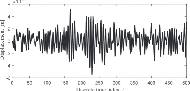
The training data shown inFig. 1was synthetically generated by integrating numerically Eq.(6)using the fourth-fifth

order Runge-Kutta method. The duration of measurements isT¼5 s with sampling frequencyf0¼100 Hz, so that the

num-ber of data points isn¼500.Table 1gives the true values used to generate the training data and their respective ranges.

Once the data has been generated, the ABC-NS algorithm illustrated in Algorithm 2 was applied to infer the model

param-eters. It is important to note that an appropriate final tolerance

e

may be difficult to specify a priori. In this example, one

considers that the convergence is met when the difference between two successive tolerance threshold values is less than

10 3. Finally, the normalised mean square error (MSE) given by Eq.(7)is selected as a metric to measure the discrepancy

between the observed and simulated data:

D

ðz

;zÞ ¼100

n

r

2

z

X n

i¼1

z

i zi 2

ð7Þ

wherenis the size of the training data,

r

2

zis the variance of the observed displacement;zandzare the observed and

sim-ulated displacements given by the model, respectively.

To be equivalent to ABC-NS, one considers for the implementation of the ABC-SMC algorithm, a percentage of alive

par-ticles

a

0¼0:6. We set the sequence of tolerance levels obtained by ABC-NS for the ABC-SMC algorithm. A proposal PDF is

assumed to be Gaussian to run the ABC-SMC algorithm (see[40], for more details).

To make a comparison between the ABC-NS and ABC-SMC algorithms, one focuses on the acceptance rate over the pop-ulations (measured by dividing the number of particles required to replenish a population by the total number of

simula-tions) together with the quality of the posterior. FromFig. 2, one can see that the ABC-NS algorithm outperforms the

ABC-SMC algorithm in terms of computational efficiency. The ABC-NS algorithm gives an acceptance rates for each

[image:6.544.110.439.514.671.2]

tion (population) in the range of 60–70%, while with the ABC-SMC, the acceptance rate decreases over the populations, it

stabilises around 35%after few populations.

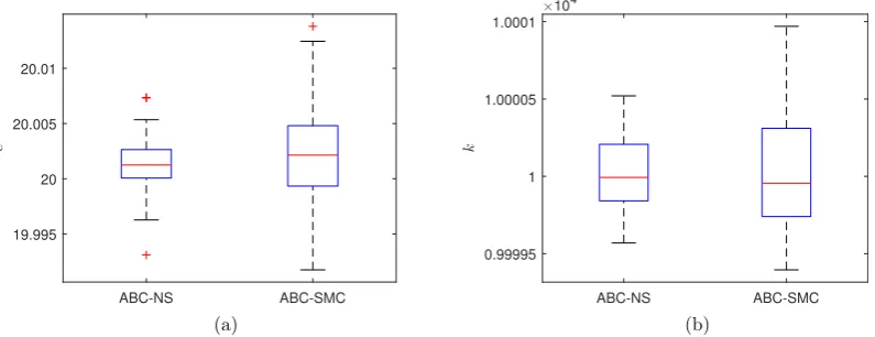
The ABC-NS and ABC-SMC results show that the mean estimates of the approximate posterior distribution is close to the

true parameters.Fig. 3displays a comparison between the posterior estimates based on 50 repeated runs of ABC-NS and

ABC-SMC. One can see that the ABC-NS achieves the same or better results in terms of accuracy with less variation on the posterior estimates.

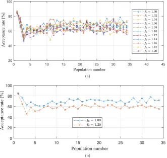
Next, one investigates the effects of the hyperparameters (f0;

a

0andb0) on the computational and statistical efficiencies.

Fig. 4a shows the effect off0on the acceptance rate, it should be noted that the pairð

a

0;b0Þis set to (0.3, 0.6). One can see

fromFig. 4a and b that by varyingf0from 1 to 1.2 impacts slightly the acceptance rate over the populations. For all the values

off0and after few populations, the acceptance rates oscillates between 60 and 70 per cent. Overall and based on Fig. 5a and

b, one can say that the effect on the posterior estimates is as well negligible.

Now, one examines the effects of the pairð

a

0;b0Þon the computational and statistical efficiencies of the ABC-NS

algo-rithm.Fig. 6shows the acceptance rate over the populations for 5 pairs. To run simulations, the value off0is set to 1.1. From

the same figure, one can see that when the value of

a

0is low (i.e., the value ofb0is high), the acceptance rate is high,

how-ever, several populations are required to ensure convergence. On the other side, a high value of

a

0is associated to a low

[image:7.544.167.373.66.285.2]

acceptance rate which is expected as we need more particles to replenish the population. We believe that the best solution Table 1

Parameter ranges of the linear model.

Parameter True value Lower bound Upper bound

c 20 10 50

k 104 5000 15000

[image:7.544.73.471.521.674.2]

Fig. 2.Acceptance rates over populations: ABC-NS vs. ABC-SMC.

is a trade-off between the rejected and the remained particles at each population. In our case studies, the values of

a

0andb0

are set to 0.3 and 0.6, respectively.

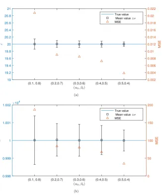
Fig. 7a and b show the evolution of the mean values (

r

) ofcandkfor the 5 different pairs. One can see that for the dif-ferent pairs, the posterior estimates are quite similar. The mean squared error (MSE) (computed using the following formula: (1

n Pn

i¼1ðhi htrueÞ) for the inferred parameters are shown on the same figures. One can see that the evolution of the MSE

val-ues shows the same tendency for both parameters. The MSE is high when the value of

a

0is low which means that from

pop-ulation to poppop-ulation a few new particles are injected. The MSE is at lowest value when

a

0is high which means a more

‘‘good” particles have been added to the population. However, as one can see from the previous figure, the acceptance rate

is low when the value of

a

0is high.

[image:8.544.110.442.54.368.2]

In this example, a brief discussion on the effects of each hyperparameter on the statistical and computational efficiencies is given. One can say that a good choice of the hyperparameters is the one who guarantees the best trade-off between the

Fig. 4.(a) The effect off0on the acceptance rate, (b) as for (a) only for the low and high values off0.

[image:9.544.110.437.252.646.2]

Fig. 6.Acceptance rates over populations: the effect of the pair (a0;b0).

computational and the statistical efficiencies. Of course, a finer study is required to provide a general guideline to the user to define those hyperparameters.

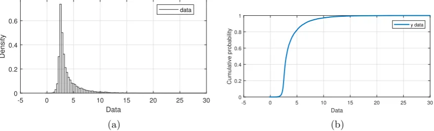
3.2. Example 2: parameter estimation of the g-and-k distribution

To demonstrate the efficiency of the ABC-NS for parameter estimation, the case study of theg-and-kdistribution is

pre-sented. Such a distribution has also been used for testing several ABC approaches as in[41–43]. This distribution can model

many types of behaviour through just a small number of parameters, and offers an ideal alternative to complex convolutions

of ‘‘regular” distributions. Theg-and-kdistribution is defined by its cumulative distribution function and no explicit

likeli-hood function is available. Theg-and-kdistribution, has four parameters describing location, scale, skewness and kurtosis

and is thus able to model many asymmetric distributions. The quantile function of theg-and-kdistribution (inverse

distri-bution function) is given by:

F 1ðX;A;B;c;g;kÞ ¼AþB 1þc1 expð grðXÞÞ 1þexpð grðXÞÞ

ð1þr2_ðXÞÞk_{rðXÞ ð8Þ}

whererðXÞis therðXÞth standard normal quantile,AandBare location and scale parameters andgandkare related to

skew-ness and kurtosis.

h¼ ðA;B;g;kÞis the vector of distribution parameters; given thatcis kept fixed toc¼0:8 following Rayner and

MacGil-livray[44](the parametercmeasures the overall asymmetry). It is noted that the normal distribution is a special case of the

g-and-kdistribution, withg= 0 andk= 0. Parameter restrictions areB>0 andk> 0:5. An evaluation of Eq.(8)returns a

draw (X-th quantile) from theg-and-kdistribution.

We follow the simulation set up for datay1;. . .;ynof sizen¼10

4

generated as in[41]withh¼ ð3;1;2;0:5Þ.Fig. 8a and b

show the histogram and the empirical distribution function of the data, revealing a peaked distribution with a long right-hand tail. Actually, it is extremely simple to obtain accurate inference for all parameters by reducing the dimensionality

of the problem as in[43]using a smaller set of summaries. It is assumed here thatSðyÞ ¼ ðP20;P40;P60;P80;skewðyÞÞas in

[43], that is the 20–40-60-80th percentiles of the data and the sample skewness. A uniform priorUð0;10Þon each parameter

is considered. The objective now is to estimate parameters with summariesSðyÞ ¼ ðyð1Þ;. . .;yðnÞÞ(the sequence of ordered

data) using the metric given by Eq.(9)to measure the degree of similarity:

Jðy;zÞ ¼ X

n

i¼1

½SiðzÞ Siðyފ2 !ð1=2Þ

ð9Þ

withSithei-th element ofSandz¼ ðz1;. . .;znÞa vector of samples from theg-and-kdistribution.

3.3. Results

To retrieve the unknown parameters, one uses the ABC-NS algorithm as illustrated in Algorithm 2. The hyperparameters

used to run the ABC-NS are defined as follows:

a

0¼0:3;b0¼0:6;f0¼1:1;N¼1000 and the convergence criterion is set

when the difference between two consecutive tolerance threshold values is less than 10 5_{. The tolerance level}

_e

_{has been}

chosen in a recursive way: first a very large value (equal to 100) has been selected and then the next value is defined based

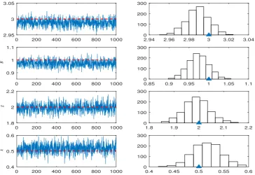
on the distances obtained in the previous population as illustrated in Algorithm 2.Fig. 9shows the marginal posterior

[image:10.544.56.496.541.674.2]

dis-tributions at the last population when the tolerance value is equal to

e

¼0:0074.

FromTable 5, one can see that ABC-NS provides a good inference of the distribution parameters. The 95%credible inter-vals for the posterior distribution of all parameters contain the true values. This example shows that by selecting a suitable set of summary statistics, one can provide a good estimates of the model parameters. From the obtained results, one can see

thatgis identifiable with high uncertainty compared with the other parameters of the distribution, mainly for the first two

tolerance values. It should be noted that it is possible to further reduce the uncertainty in the distribution parameters by decreasing the final tolerance threshold, of course by introducing computational cost.

The second example illustrates the statistical efficiency of the ABC-NS in dealing with parameter estimation from data. One can see how, by selecting an appropriate summary statistics, one can efficiently make Bayesian inference circumventing

the issue of intractable likelihood functions. In the rest of this paper, the efficiency of the ABC-NS to deal withmodel selection

[image:11.544.90.455.52.302.2]

is investigated through two examples using simulated and real data. (Table 2).

Fig. 9.(left)g-and-kdistribution: trace plots for the ABC-NS run at the last population, (right) marginal posterior distributions of theg-and-kdistribution parameters, (the blue triangles show the true values).

Table 2

Posterior estimates for theg-and-kdistribution parameters at different target tolerance values.

Tolerance value Parameter Posterior estimates

Mean Std dev ½2:5%;97:5%Špercentiles

e¼0:1345 A 2.9615 0.0573 [2.9313, 3.0587]

B 0.9839 0.0458 [0.9499, 1.0712]

g 2.5434 1.5117 [1.9146, 9.3087]

k 0.4964 0.0402 [0.4689, 0.5740]

e¼0:0444 A 2.9842 0.0201 [2.9702, 3.0230]

B 0.9873 0.0332 [0.9653, 1.0528]

g 2.0383 0.1317 [1.9406, 2.2894]

k 0.4970 0.0374 [0.4715, 0.5688]

e¼0:0169 A 2.9869 0.0129 [2.9777, 3.0113]

B 0.9794 0.0283 [0.9614, 1.0335]

g 2.0064 0.0648 [1.9604, 2.1281]

k 0.5085 0.0330 [0.04858, 0.5754]

e¼0:0074 A 2.9888 0.0115 [2.9815, 3.0114]

B 0.9738 0.0257 [0.9568, 1.0237]

g 1.9906 0.0515 [1.9569, 2.0980]

[image:11.544.36.506.511.691.2]

4. ABC-NS for model selection using Duffing-type oscillators

4.1. Example 1: cubic and cubic-quintic models

The performance of the ABC-NS algorithm is now investigated for model selection by considering two candidate models:

the cubic and cubic-quintic Duffing oscillators denoted byM1andM2, respectively. The equation of motion associated to

each model is given by:

M1: €zþcz_þkzþk3z3¼fðtÞ ð10Þ

M2: €zþcz_þkzþk3z3þk5z5¼fðtÞ ð11Þ

wherecis the damping,kis the linear stiffness,k3andk5are the non-linear stiffness coefficients.z;z_and€zare displacement,

velocity and acceleration responses, respectively. The excitationfðtÞis a Gaussian sequence with mean zero and standard

deviation of 10.

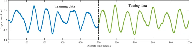
To make Bayesian inference, a noisy training data set was generated from the cubic-quintic model and shown inFig. 10

(the first 500 data points). It has been corrupted with Gaussian noise of standard deviation 1%RMS. The fourth and

fifth-order Runge-Kutta algorithm is chosen to integrate the equations of motion. To evaluate the model predictability, a set of

testing data has been generated shown inFig. 10(the second 500 points).Table 3summarises the prior lower and upper

bounds associated to each unknown parameter of the competing models.

For the ABC-NS implementation, the same scheme shown in Algorithm 2 is followed by considering the candidate models

as additional parameters. One sets the prior probabilities of each model to be equal, i.e.,pðM1Þ ¼pðM2Þ ¼12. In the ABC-NS

for model selection, one treats the pairðMk;hðkÞÞwithMkas a candidate model andhðkÞits vector of unknown parameters.

For a givenðMk;hðkÞÞ, the pair is accepted or rejected based on a discrepancy value. At the end of the algorithm, the model

probability forMkis approximated using Eq.(12).

pðMkjuÞ

Accepted particles forMk

Total number of particlesN ð12Þ

The convergence criterion used here is when the difference between two successive tolerance values is less than 10 7

(

e

ðjÞ

e

ðjþ1Þ<10 7; jisthepopulationnumber). For the rest, the same hyperparameters defined earlier have been used.

It should be noted that the number of the dropped and remaining particles are rounded to the nearest integer in each step

of the algorithm such that the sum of the dropped and new particles is equal toN. Finally, the normalised mean square error

(MSE) given by Eq.(7)and used in the first example is selected as a metric to measure the discrepancy between the observed

and simulated data.

4.2. Results and discussion

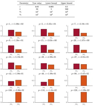
Fig. 11shows the model posterior probabilities over a selected number of populations. One can see how the ABC-NS algo-rithm oscillates between the competing models and finishes by converging to the correct model when the tolerance values become very small. From the same figure, one can see that the algorithm clearly tries first to favour the cubic model, this can be seen from populations 1 to 37. Then, when the cubic model is no longer able to match the data very well, the ABC-NS algorithm jumps to the complex model to accommodate the nonlinearity coming from the quintic term. The probability of selecting this ‘‘true” model approaches when the tolerance value is very small and close to zero. This demonstrates that

the parsimony principle[45]is well embedded in the ABC-NS algorithm by favouring first simpler models. As mentioned

earlier, in the classical methods based on the evaluation of an information criterion, overly-complex models are penalised

through anad hocpenalty term while the ABC algorithm naturally favours simpler models as shown here, which is a major

[image:12.544.75.473.575.673.2]

advantage circumventing the issue of which information criterion is more suitable to compare models.

[image:13.544.108.436.69.443.2]

Fig. 12shows the acceptance rate over the populations, one can see how the ABC-NS algorithm maintains a relatively high acceptance rate over the populations. At early populations, the acceptance rate decreases because the input space to be explored is large, then steadily rises as the volume of the search space shrinks down. From population 30 to population

Table 3

Parameter ranges of the competing models.

Parameter True value Lower bound Upper bound

c 0.05 0.005 0.5

k 50 5 500

k3 103 102 104

k5 105 104 ₁₀6

[image:13.544.107.434.476.622.2]

Fig. 11.Model posterior probabilities considering the cubic and cubic-quintic models.

[image:14.544.108.440.435.676.2]

81, it stabilises around an average value higher than 35 per cent and then decreases as a finer representation of the data is required at that stage until the elimination of the cubic model (population 91). Then, from population 91, the acceptance rate rises again as the search domain for the selected model is well defined.

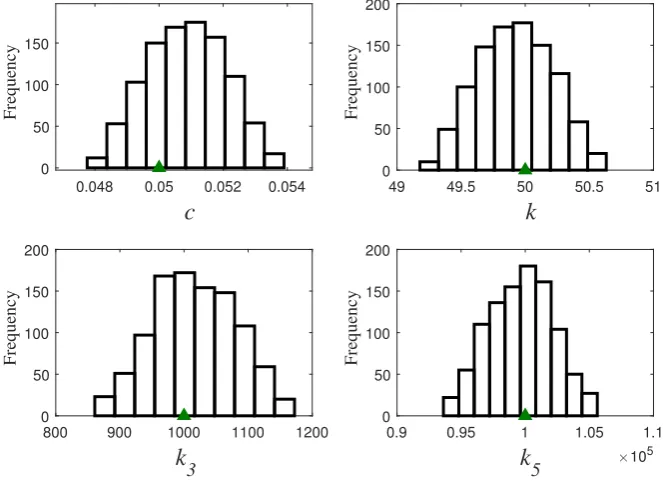
Fig. 13shows the histograms of the unknown parameters associated to the cubic-quintic model obtained at the last

pop-ulation. One can see how the histograms are well peaked around the true values.Table 4summarises the statistics of the

posterior estimates associated with the selected model. The estimated model parameters are then used to make future

pre-dictions and evaluate the model predictability. FromFig. 14, it can be seen that the training and testing data sets are well

predicted. The 99%confidence interval is found pointwise by generating randomly a large number of samples, simulating

the model responses and then the 99%confidence interval is found pointwise. The normalised MSE estimated on the first

500 data points is equal to 0.2580 and is 0.4698 on the testing data. Based on[2], the discrepancy measure formulated in

Eq.(7)has shown that a value less than 5 generally indicates a good fit while a value less than 1 means an excellent fit.

It should be noted that the obtained posterior estimates could be easily refined and therefore reduce the uncertainty on the parameters by further decreasing the final tolerance threshold value. The main advantage of the ABC-NS algorithm in comparison with its predecessors is that this can be done at low computational cost as the region from where one can sam-ple a ‘‘good” candidates is well delimited by the ellipsoids.

Finally, in order to check the repeatability of the model posterior probabilities, the ABC-NS algorithm is run 20 times. FromFig. 15, one can see how the ABC-NS produces repeatable results with small variations. Clearly the algorithm tries first to favour the simpler model (here the cubic model) (see the model posterior probabilities at populations 1, 11, 31, 51, 76 and 91) and when a higher predictive performance is required then the algorithm switches to the more complex model to justify the increase in complexity. In short, a simpler (but equally accurate) explanation for data always has the greater evidence.

5. Characterisation of the dynamics of a wire rope isolators using ABC-NS

5.1. Experimental set-up

The last system consists of characterising the dynamics of a wire rope isolator (WRI) used for vibration isolation. WRIs have found a vast number of application in medical equipment, mechanical machinery, and military hardware due to their superior performance for the isolation of impact and vibration. However, the dynamical properties of mechanical isolators are typically non-linear and these characteristics are seldom well defined, which may cause problems for design calculation and computer simulations. The system considered in this paper has been proposed within the framework of the European

COST Action F3 working group in ‘‘Identification of non-linear systems”[46]. The aim of this benchmark was to identify the

dynamic properties of resilient mounts used for vibration isolation in industrial applications using different methods. Fig. 16a shows the experimental set-up of the WRI mounted between a load massm2and a base massm1bwhileFig. 16b is a schematic illustration. The excitation produced by an electro-dynamic shaker corresponds to a white noise sequence,

low-pass filtered at 400 Hz. The motion and forces experienced by the isolators are measured; in particular, the acceleration

responses€x2and€x1bof the load mass and bottom plate, the appliedfand the relative displacementx12between the top and

bottom plates. Five excitations ranging from 0.5 up to 8 V have been considered. For more details concerning the experimen-tal set-up and the methods presented for the identification of the system, the reader is referred to the following references [49,50,47,48].Table 5illustrates the characteristics of the testing system and the WRI properties.

Wire rope isolators have different response characteristics depending on the selected properties mentioned inTable 5. To

determine their dynamic characteristics, a series of dynamic tests were conducted by imposing a random excitation at dif-Table 4

Posterior estimates for the cubic-quintic model parameters.

Parameter True value Posterior estimates

Mean,l Std. Dev,r [5th, 95th] percentiles

c 0.05 0.05086 1:2167103 _[1:87

10 2

;5:282710 2_]

k 50 49.9211 2:8995101 _{[49:4382;50:3844]}

k3 103 _{1016.5110 63:8396 [914:045;1123:6337]}

k5 105 _9:9670

104 _2:5015

103 _[9:5183

104_;1:036

[image:15.544.43.491.84.274.2]

105_]

Fig. 14.Model prediction using the cubic-quintic model on training and testing data sets.

[image:15.544.42.496.308.585.2]

ferent excitation levels. Random excitation consists of a white noise, low-pass filtered (LPF) (18 db/oct) at 400 Hz. Different levels of excitation were produced and the time signals were recorded with a sampling frequency of4096 Hz. As an example,

the displacement and inertial force versus relative displacement for three levels of excitation are shown in Fig. 17a–f.

Recorded inertial force-relative displacement loops showed hysteretic behaviour for all five amplitudes (only three of them are shown for brevity). A hysteretic behaviour can be seen which means that a hysteretic model could potentially describe the data reasonably well.

5.2. Selection of the candidate models

For the competing models, one selects the linear model given by the following expression as a competing model:

my€þcy_þAy¼xðtÞ ð13Þ

whereðm;c;AÞare the parameters to be identified andxðtÞis the applied excitation.

It should be noted that the linear model is selected on purpose to analyse the behaviour of the algorithm and to inves-tigate if this model could be used to describe the dynamics of the WRI, mainly at low excitation levels. To describe the hys-teretic behaviour of the WRI, a well developed mathematical model of hysteresis would be useful to make predictions and avoids the time-consuming experimental work. In this study, the Bouc-Wen model is used to model the hysteretic beha-viour. Many researchers have used the Bouc-Wen model to perform mathematical modelling of the hysteresis system in

sev-eral areas including hysteretic isolators[51,52]. The Bouc-Wen model of hysteresis is given by:

my€þgðy;y_Þ þzðy;y_Þ ¼xðtÞ ð14Þ

wheremis the mass of the system,gðy;y_Þ ¼cy_þkyis the polynomial part of the restoring force,zðy;y_Þis the hysteretic part

andxðtÞis the excitation force.

[image:16.544.53.493.54.253.2]

The hysteretic component is defined by Wen[53]via an additional equation of motion:

Fig. 16.(a) Experimental set-up: schematic configuration of the experiment, (b) illustration of the dynamical system under consideration[50].

Table 5

System characteristics and geometrical properties of helical wire rope isolators.

System characteristics

Load mass,m2 2.2 kg

Bottom plate,m1b 1.1 kg

Shaker base 3.7 kg

Wire diameter 2 mm

Length 110 mm

Number of loops 10

[image:16.544.127.427.308.388.2]

_

z¼

a

jy_jz

n _{by_jz}n_{j þAy;_ fornodd}

a

jy_jzn 1_{jzj by_jz}n_{j þAy;_ forneven}

ð15Þ

where (c;

a

;b;A) are the parameters to be identified,nis a discrete parameter.

The parameters (A;

a

;b) govern the shape and smoothness of the hysteresis loop. The equations offer a simplification from

the point of view of parameter estimation in that the stiffness term in Eq.(14)can be combined with the termAin the state

equation forz. The coupled Eqs.(14) and (15)were integrated forward in time using fourth-order Runge-Kutta integration.

In total, five competing models will be considered to perform model selection using ABC-NS: the linear model given by Eq.

(13)and hysteretic models (Eqs.(14) and (15)) by varyingnfrom 1 to 4. The priors assigned to the model parameters are

given inTable 6. All other settings for the ABC-NS algorithm were specified as before.

[image:17.544.69.469.57.419.2]

In the first part of this example, one aims to select the most likely model among the competing ones for each excitation amplitude. The data set contains 1000 samples representing a short recording period of the acceleration of the top plate. The

Fig. 17.Displacement and inertial force versus relative displacement under excitation levels of (a, b) 8 V, (c, d) 4 V and (e, f) 2 V.

Table 6

Priors on model parameters.

Parameter Lower bound Upper bound

c 103 ₁₀3

k 105 ₁₀6

a 104 105

b ₁₀4

105

[image:17.544.193.349.621.690.2]

data set is split into training data (from 501 to 1000) and testing data (from 1001 to 1500) as shown inFig. 18. It should be noted that the transient part (from 0 to 500) has been ignored in computing the MSE, to reduce the effect of initial conditions.

5.3. Results and analyses

Following the same scheme as before, the ABC-NS for model selection is implemented by assuming the same prior

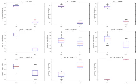
prob-ability to the competing models.Fig. 19shows the model posterior probabilities over some selected populations. One can see

that the most likely model isM2. As before, one can see that the parsimony principle is deeply embedded in the ABC-NS

[image:18.544.74.474.57.158.2]

algorithm. It tries firstly to select the simpler models and then when those models are not able to describe the dynamics due the complexity of the data and the presence of nonlinearity, then the algorithm jumps to a more sophisticated model. Table 7summarises the statistics of model parameters for the selected excitation levels from where one can see that the

Fig. 18.Training and testing data sets using an excitation of amplitude 8 V.

[image:18.544.82.463.332.673.2]

[image:19.544.43.490.80.332.2]

parameters have been estimated with a reasonable amount of uncertainties.Fig. 20shows the model prediction on the train-ing and testtrain-ing data sets from where one can see a good agreement.

Fig. 21shows how the ABC-NS maintains a high acceptance rate over the populations required for convergence. This reduces considerably the computational time to converge to the most likely model.

The same procedure is now applied for the rest of the data sets for all the excitation levels to determine the most likely

models. The Bayesian inference using ABC-NS with the same hyperparameters as earlier is performed.Table 8shows the

most likely model for each data set and the MSE estimated on the training and testing data sets.Table 9shows the statistics

of the model parameters from which, one can see as before, a reduced amount of uncertainty on the parameters. Model

pre-diction for excitation 4 V is shown inFig. 22, where one can see a good correlation between real and simulated data on

train-ing and testtrain-ing data sets. A good agreement is shown as well for the other excitation levels not shown here for brevity. The obtained results show that the Bouc-Wen model describes reasonably well the dynamics of the WRI. One point should be noted that the selection of the appropriate model varies with the excitation level which is not desirable mainly Table 7

Posterior estimates using an excitation amplitude of 8 V.

Excitation Moments Model parameters

level c a b A

8 V l 78.7315 3:9135103 _1:5644104 _3:3328105

r 0.2414 29.2111 97.9579 4:6459102

[image:19.544.107.435.517.672.2]

Fig. 20.Model prediction under excitation amplitude 8 V.

when the practitioner needs one model to describe the dynamics of the WRI independently of the excitation level. This point is addressed in the next subsection where the objective is to select one model which performs better considering all the

test-ing data sets and all the excitation levels simultaneously. To answer this question, one uses aconfusion matrixintroduced and

widely used in machine learning.

Before closing this section, one important point should be highlighted at low excitation levels (0.5 V, 1 V and 2 V). It has been noticed that the linear model is favoured at the beginning of the algorithm and has been eliminated at an advanced

stage, as can be seen fromFig. 23(at population 26 with

e

¼0:812). This leads one to think that the system behaviour might

be predominantly linear, though the algorithm converges to one of the hysteretic models when the performance require-ment in terms of prediction is high. To confirm this result, one uses the linear model to check its ability to make predictions. Figs. 24 and 25show that using the linear model at two different tolerance threshold values, an acceptable agreement is

shown between the predicted and simulated data (inFig. 25, the 99%CI is not shown as it is indistinguishable from the

model prediction).

5.4. Confusion matrix

[image:20.544.45.510.73.135.2]

Although model selection can be straightforwadly performed for each excitation amplitude alone. The practitioner may prefer one single model which can be used to describe the dynamics of the isolator regardless of the excitation level. In such Table 8

Normalised MSE evaluated on training and testing data using mean posterior estimates.

Excitation amplitude (V) Selected model Training data Testing data

8 M2 1.4010 2.4538

4 M2 0.7787 0.6338

2 M3 0.1783 0.2782

1 M5 0.1848 0.3368

[image:20.544.44.507.183.304.2]

0.5 M4 0.5550 0.9999

Table 9

Posterior estimates using the other excitation amplitudes.

Excitation level (V) Moments Model parameters

c a b A

4 l 70.9807 1:7234103 _3:3253

104 _4:5797105

r 0.1400 12.9543 58.2083 2:4260102

2 l 41.2794 1:1003103 _2:9893104 _4:7203105

r 0.2280 90.9088 1:7992102 _3:1932102

1 l 29.6899 4:1047103 _2:6767104 _4:7829105

r 0.1537 88.9378 1:8534102 _2:0254102

0:5 l 3.0524 _3:4739104 _1:7453104 _4:5444105

[image:20.544.59.480.249.468.2]

r 0.1422 1:8659102 _3:0277102 _1:5292102

cases, a problem may arise of deciding which of the competing models can provide acceptable predictions considering all the

testing data sets. To answer this challenging question, one introduces theconfusion matrix, a concept widely adopted in

machine learning as mentioned earlier. The objective behind its use is to train the model considering one amplitude and then quantify the performance of the model prediction based on the same metric (normalised MSE) using the rest of the testing

data sets as illustrated inFig. 26. The confusion matrix is given below for a better understanding of its use in this context.

[image:21.544.105.439.52.257.2]

This allows one to give a clear idea of how each model performs considering all the testing data sets. Then, the selection of the best model is done straightforwadly based on a comparison of the MSE values considering all the testing data sets.

[image:21.544.107.435.299.415.2]

Fig. 23.Evolution of the model posterior probabilities over the populations using an excitation amplitude of 0.5 V.

Fig. 24.Model prediction using the linear model under an excitation amplitude of 0.5 V (e¼5:44).

[image:21.544.110.435.455.571.2]

[image:22.544.173.377.56.181.2]

Fig. 27gives the confusion matrices associated to the competing models. One can clearly see thatMn¼2

3 is the best model

considering all the testing data sets based on the MSE values. This means that this model generalises better under different excitation levels and should be selected if the practitioner prefers one model rather than a model for each excitation

ampli-tude. The confusion matrix associated toM5is not shown here as it shows some numerical instability and therefore it has

been eliminated from the competition.

Based on these results, one may conclude that the Bouc-Wen model is a good way for describing the hysteretic behaviour of the WRI. It has been shown that this model is efficient and has a good performance in terms of prediction under different excitation amplitudes. Overall, the simulated data were in good agreement with experimental results.

[image:22.544.68.477.342.668.2]

Fig. 26.The confusion matrix concept.

6. Conclusions

A new approximate Bayesian computation algorithm based on an ellipsoidal nested sampling method named ABC-NS has been proposed in this paper for parameter estimation and model selection. It has been shown through four examples using simulated and real data how the ABC-NS outperforms the popular ABC-SMC and overcomes the low efficiency observed after few iterations by employing a more sophisticated technique to generate new samples. ABC-NS maintains a high acceptance rate over the populations, which speeds up considerably the algorithm without compromising the precision of the posterior estimates. As a result, significant savings in computational effort can be achieved, which is desirable particularly to enable larger models to be analysed, the use of more computationally intensive forward simulation models and the inclusion of additional uncertain parameters. Moreover, as it has been shown, the parsimony principle is naturally embedded in the ABC algorithm. The ABC tells one which models are supported by the data in a straightforward way without any additional cost. In conclusion, likelihood-free or approximate Bayesian computation algorithms represent a simple and efficient way to handle highly complicated problems. It is extremely useful mainly when the likelihood function is intractable or cannot be approached in a closed form offering the possibility to make Bayesian inference by using different kinds of features and met-rics representative of the data.

Acknowledgement

The support of the UK Engineering and Physical Sciences Research Council (EPSRC) through grant reference No. EP/ K003836/1 is greatly acknowledged.

References

[1]G.E. Box, N.R. Draper, Empirical Model-Building and Response Surfaces, Wiley, New-Work, 1987.

[2]K. Worden, J.J. Hensman, Parameter estimation and model selection for a class of hysteretic systems using Bayesian inference, Mech. Syst. Signal Process. 32 (2012) 153–169.

[3]Ph. Bisaillon, R. Sandhu, M. Khalil, C. Pettit, D. Poirel, A. Sarkar, Bayesian parameter estimation and model selection for strongly nonlinear dynamical systems, Nonlinear Dyn. 82 (2015) 1061–1080.

[4]J.L. Beck, K.V. Yuen, Model selection using response measurements: Bayesian probabilistic approach, J. Eng. Mech. 130 (2) (2004) 192–203. [5]R. Sandhu, M. Khalil, A. Sarkara, D. Poirel, Bayesian model selection for nonlinear aeroelastic systems using wind-tunnel data, Comput. Methods Appl.

Mech. Eng. 282 (2014) 161–183.

[6]J.L. Beck, S.K. Au, Bayesian updating of structural models and reliability using Markov chain Monte Carlo simulation, J. Eng. Mech.- ASCE 128 (2002) 380–391.

[7]J.Y. Ching, Y.C. Chen, Transitional Markov chain Monte Carlo method for Bayesian model updating, model class selection, and model averaging, J. Eng. Mech. ASCE 133 (2007) 816–832.

[8]C. Soize, Bayesian posteriors of uncertainty quantification in computational structural dynamics for low-and medium-frequency ranges, Comput. Struct. 126 (2013) 41–55.

[9]K.V. Yuen, Bayesian Methods for Structural Dynamics and Civil Engineering, John Wiley & Sons, 2010.

[10] H. Akaike, Information theory and an extension of the maximum likelihood principle, Breakthroughs in Statistics, vol. I, Springer, 1992, pp. 610–624. [11]G. Schwarz et al, Estimating the dimension of a model, Ann. Stat. 6 (2) (1978) 461–464.

[12]D.J. Spiegelhalter, N.G. Best, B.P. Carlin, A. van der Linde, Bayesian measures of model complexity and fit, J. R. Stat. Soc. Ser. B (Methodol.) 64 (4) (2002) 583–639.

[13]P.J. Green, Reversible jump Markov chain Monte Carlo computation and Bayesian model determination, Biometrika 82 (4) (1995) 711–732. [14]M. Muto, L.J. Beck, Bayesian updating and model class selection for hysteretic structural models using stochastic simulation, J. Vib. Control 14 (2008)

7–34.

[15]J.Y. Ching, Y.C. Chen, Transitional Markov chain Monte Carlo method for Bayesian model updating, model class selection, and model averaging, J. Eng. Mech.- ASCE 133 (2007) 816–832.

[16]W. Betz, I. Papaioannou, D. Straub, Transitional Markov Chain Monte Carlo: observations and Improvements, ASCE J. Eng. Mech. 142 (5) (2016). [17]S. Wu, P. Angelikopoulos, C. Papadimitriou, Petros Koumoutsakos, Bayesian annealed sequential importance sampling: an unbiased version of

transitional Markov Chain Monte Carlo, ASCE-ASME J. Risk Uncertainty Eng. Syst. Part B 4 (1) (2018), 011008-1.

[18] J. Skilling, Nested sampling for general Bayesian computation, Bayesian Anal. 1 (4) (2006) 833–860,https://doi.org/10.1214/06-BA127.

[19]J. Skilling, Nested sampling, in: R. Fischer, R. Preuss, U. Toussaint (Eds.), Bayesian Inference and Maximum Entropy Methods in Science and Engineering, AIP Conference Proceedings, 735, 2004, pp. 395–405.

[20] F. Feroz, M.P. Hobson, Multimodal nested sampling: an efficient and robust alternative to MCMC methods for astronomical data analysis, Monthly Notices R. Astron. Soc. 384 (2007) 449–463.

[21]P. Mukherjee, D. Parkinson, A.R. Liddle, A nested sampling algorithm for cosmological model selection, Astrophys. J. 638 (2006) L51–L54. [22]D. Parkinson, P. Mukherjee, P. Liddle, A Bayesian model selection analysis of WMAP3, Phys. Rev. D 73 (2006) 123523.

[23]A. Ben Abdessalem, Model selection, updating and prediction of fatigue crack propagation using nested sampling algorithm, in: Conference: 23 Congrès Français de Mécanique, 2017, Lille, France.

[24]A. Ben Abdessalem, F. Jenson, P. Calmon, Quantifying uncertainty in parameter estimates of ultrasonic inspection system using Bayesian computational framework, Mech. Syst. Signal Process. 109 (2018) 89–110.

[25]M.A. Beaumont, W. Zhang, D.J. Balding, Approximate Bayesian computation in population genetics, Genetics 162 (4) (2002) 2025–2035. [26]B.M. Turner, T. Van Zandt, A tutorial on approximate Bayesian computation, J. Math. Psychol. 56 (2012) 69–85.

[27] A. Ben Abdessalem, N. Dervilis, D. Wagg, K. Worden, Automatic kernel selection for Gaussian processes regression with approximate Bayesian computation and sequential Monte Carlo, Front. Built Environ. 3:52 (2017),https://doi.org/10.3389/fbuil.2017.00052.

[28]M. Chiachio, J.L. Beck, J. Chiachio, G. Rus, Approximate Bayesian computation by subset simulation, SIAM J. Scientific Comput. 36 (3) (2014), A1339-A1338.

[29] A. Ben Abdessalem, N. Dervilis, D. Wagg, K. Worden, Identification of nonlinear dynamical systems using approximate Bayesian computation based on a sequential Monte Carlo sampler, in: International Conference on Noise and Vibration Engineering, September 19-21, 2016, Leuven (Belgium). [30] M.K. Vakilzadeh, J.L. Beck, T. Abrahamsson, Using approximate Bayesian computation by subset simulation for efficient posterior assessment of

[31]A. Ben Abdessalem, N. Dervilis, D. Wagg, K. Worden, Model selection and parameter estimation in structural dynamics using approximate Bayesian computation, Mech. Syst. Signal Process. 99 (2018) 306–325.

[32]A. Ben Abdessalem, N. Dervilis, D. Wagg, K. Worden, ABC-NS: a new computational inference method applied to parameter estimation and model selection in structural dynamics, in: Conference: 23 Congrès Français de Mécanique, 2017, Lille, France.

[33]P. Marjoram, J. Molitor, V. Plagnol, S. Tavare, Markov chain Monte Carlo without likelihoods, Proc. Natl. Acad. Sci. U.S.A. 100 (2003) 15324–15328. [34]S. Sisson, Y. Fan, M. Tanaka, Sequential Monte Carlo without likelihoods, Proc. Natl. Acad. Sci. U.S.A. 104 (2007) 1760–1765.

[35]T. Toni, D. Welch, N. Strelkowa, A. Ipsen, M.P.H. Stumpf, Approximate Bayesian computation scheme for parameter inference and model selection in dynamical systems, J. R. Soc. Interface 6 (2009) 187–202.

[36]F.V. Bonassi, Approximate Bayesian Computation for Complex Dynamic Systems (Ph.D. thesis), Duke University, 2013.

[37]F.V. Bonassi, M. West, Sequential Monte Carlo with adaptive weights for approximate bayesian computation, Bayesian Anal. 10 (1) (2015) 171–187. [38]F. Feroz, M.P. Hobson, M. Bridges, MultiNest: an efficient and robust Bayesian inference tool for cosmology and particle physics, Monthly Notice R.

Astron. Soc. 398 (4) (2009) 1601–1614.

[39]J.R. Shaw, M. Bidges, M.P. Hobson, Efficient Bayesian inference for multimodal problems in cosmology, Monthly Notice R. Astron. Soc. 000 (2006) 1–7. [40]E. Jennings, M. Madigan, astroABC: an approximate bayesian computation sequential Monte Carlo sampler for cosmological parameter estimation,

Astron. Comput. 19 (2017) 16–22.

[41]D. Allingham, R.A.R. King, K.L. Mengersen, Bayesian estimation of quantile distributions, Stat. Comput. 19 (2009) 189–201.

[42]Christopher C. Drovandi, Anthony N. Pettitt, Likelihood-free Bayesian estimation of multivariate quantile distributions, Comput. Stat. Data Anal. 55 (2011) 2541–2556.

[43]U. Picchini, R. Anderson, Approximate maximum likelihood estimation using data-cloning ABC, Comput. Stat. Data Anal. 105 (2017) 166–183. [44]G. Rayner, H. Macgillivray, Weighted quantile-based estimation for a class of transformation distributions, Comput. Stat. Data Anal. 39 (4) (2002) 401–

433.

[45]H. Walach, Ockham’s razor, in: Wiley Interdisciplinary Reviews Computational Statistics, vol. 2, Sage Publications, 2007. [46]C.O.S.T. Technical Report, Action F3, VTT Technical, Research Centre of Finland (1999).

[47]M. Juntunen, J. Linjama, Presentation of the VTT benchmark, Mech. Syst. Signal Process. 17 (1) (2003) 179–182.

[48]G. Kerschen, K. Worden, Alexander F. Vakakisc, J.C. Golinval, Past present and future of nonlinear system identification in structural dynamics, Mech. Syst. Signal Process. 20 (2006) 505–592.

[49]G. Kerschen, On the Model Validation in Non-linear Structural Dynamics (Thèse de doctorat), Université de Liège, 2002.

[50]M. Peifer, J. Timmer, H.U. Voss, Non-parametric identification of non-linear oscillating systems, J. Sound Vib. 267 (2003) 1157–1167.

[51]G.F. Demetriades, M.C. Constantinou, A.M. Reinhorn, Study of wire rope systems for seismic protection of equipment in buildings, Eng. Struct. 15 (5) (1993) 321–334.