Filter Selection for Spectral Estimation Using a Trichrmatic Camera

Rochester Institute of Technology

RIT Scholar Works

Theses

Thesis/Dissertation Collections

2003

Filter Selection for Spectral Estimation Using a

Trichrmatic Camera

David C. Day

Follow this and additional works at:

http://scholarworks.rit.edu/theses

Recommended Citation

Filter

Selection for Spectral Estimation

Using

a

Trichromatic

Camera

David Collin

Day

B.S.

Imaging

Science

Filter Selection for Spectral Estimation Using a Trichromatic Camera

By

David Collin Day

B.S. Imaging Science

Rochester Institute of Technology (200

I)

A thesis submitted

in partial fulfillment of the requirements of

for the degree of Master of Science

in the

Chester F. Carlson Center for Imaging Science of the

College of Science

Rochester Institute of Technology

October 2003

Signature of Author. _ _ _ _ _ _ _ _ _ _ _ _ _ _ _ _ _ _ _ _

_

Accepted

by _ _ _ _ _ _

--:--_---=-_ _ _

----L-/_

tJ

_----=-'l'---_O-=-.3_

CHESTER F. CARLSON

CENTER FOR IMAGING SCIENCE

COLLEGE OF SCIENCE

ROCHESTER INSTITUTE OF TECHNOLOGY

ROCHESTER, NEW YORK

CERTIFICATE OF APPROVAL

M.S. DEGREE THESIS

The M.S. Degree Thesis of David Collin Day has been

examined and approved by the thesis committee as satisfactory

for the thesis requirement for the Master of Science degree

Dr. Roy S. Berns, Thesis Advisor

Dr. Francisco H. Imai

Dr. Mark D. Fairchild

THESIS RELEASE PERMISSION

ROCHESTER INSTITUTE OF TECHNOLOGY

COLLEGE OF SCIENCE

CHESTER F. CARLSON

CENTER FOR IMAGING SCIENCE

Filter Selection for Spectral Estimation Using a Trichromatic Camera

I, David Collin Day, hereby grant

permission to the Wallace Memorial Library of R.I.T.

to reproduce my thesis in whole or in part. Any reproduction will not be for commercial

use or profit.

Signature: _ _ _ _ _ _ _ _ _ _ _ _ _

_

Date:

/0/7

!tJ3

---./f----II'---=---FilterSelection for Spectral Estimation

Using

aTrichromatic Camera

By

DavidCollin

Day

Athesissubmittedinpartialfulfillmentoftherequirements of forthedegreeofMasterofScienceinthe

Chester F. Carlson Center for

Imaging

Scienceofthe CollegeofScience

RochesterInstituteof

Technology

Abstract:

Current

imaging

practices arebasedon_exploitingmetamerismtorecord and reproduce

images. Asa_{result, the}dataobtainedintheseimagesaredependentonthe_viewing conditions andtheobserver. Whilethesemethods produce acceptable results for

day

to

day

use,

they

oftendonot exhibitthe typeof_accuracyand control requiredforscientific purposes such as art conservation. Asa_{solution, many}researchinstitutionsare now advocatingtheuseof multispectral

imaging

torecordtheobjects fundamentalspectral propertiestoremovethedata's

dependency

ontheobserver and_viewingenvironment.

Theresearchdescribedinthis thesisinvolved

determining

ifatrichromaticcamera and

readilyavailablefilterscanbeusedforspectral estimation purposes. The Pixel Physics TerraPixcamera system was_{characterized,}itsresponsetoatargetand 105Kodak

WrattenFiltersundertungstenilluminationwas_simulated,and spectral reflectance estimations were generated. The

top

filtercandidates were chosenbasedontheir simulated performance. These filterswerethenusedinan

imaging

experimentdesigned

toapproximateconditionsthatwouldbe found inan art_galleryor other place where_copy workisperformed. Theresults ofthe

imaging

experiment werecomparedwiththe simulation,and shortcomings ofthemodel wereidentified. Theresults oftheexperiment showthata camera model canbeused as a_guidingtool tomakefilterselectionsfor

Acknowledgements:

Specialthanksgoto the

following

individuals:

Dr.

Roy

S.

Berns,

_{for giving}methe_opportunitytowork onthis_{project, making}it

possible formetosee various works of artina mannerthatmost peopledonot

know_exist,and

helping

meimproveas anindividual.

Dr. Francisco H.

Imai,

who gave me

help

and_pointers,butmore

importantly

made melookat_{everything in}adifferent_manner,helpedmerealizethat things

are notasbadas

they

_seem,and_{for simply}

being

an

incredibly

supportivefriend

throughout thisentire process.

Dr. Mark D.

Fairchild,

for hisadviceand_{recommendations,}and

helping

me out

inabind.

Lawrence

Taplin,

for_spendingtime_{answering my questions,}

helping

meimprove

my writingandresearch_techniques,and

listening

to_myproblems and concerns.

Allthepeople attheMunsellColor Science

Laboratory,

whohaveat one point or

another given me ahand.

My

sponsors,theMellon

Foundation,

theNational

Gallery

of

Art,

Washington

D.C.,

theMuseumofModern

Art,

New York

City,

andPixel Physicsfortheir generous

funding

and use of equipment which madethis thesispossible.

My

parents,for

being

therewhenIneededthemmost.

Taryn,

forallher_patience,support and_makingmefeel likesomeone whenIfelt likeIwasnothing.

Table

of

Contents:

TableofContents: vii

ListofFigures: ix

ListofTables: xiv

MunsellColor Science

Laboratory

Spectral Notation: xv

Chapter 1 - Introduction

andOverview: 1-1

Introduction: 1-1

Overview: 1-6

Chapter 2- Spectral

Imaging

Systems Background: 2-1

Narrowbandcapture: 2-1

Widebandcapture: 2-2

Trichromaticcamera with absorptionfilters: 2-3

Conclusions: 2-4

Chapter 3- Equipment: 3-1

Purpose: 3-1

Pixel Physics TerraPixcamera system: 3-1

Elinchrome ScanliteDigital 1000: 3-2

Targets: 3-3

Filters: 3-6

Processing: 3-7

Chapter4- Filter Selectionfor Spectral

Estimation usingaNoiselessCameraModel:.4-1

Purpose: 4-1

FilterSelectionMethod: 4-1

SpectralReconstruction Theory: 4-2

Experimental: 4-4

ResultsandDiscussion: 4-9

Conclusions: 4-22

Chapter5

-Modeling

theCamera Noise for Simulation: 5-1

Purpose: 5-1

Noise Sources: 5-2

Experimental: 5-3

ModelResults: 5-13

Conclusions: 5-17

Chapter6- Filter Selectionfor SpectralEstimation

Incorporating

aNoiseModel: 6-1

Purpose: 6-1

Theory

ofSpectralReconstruction usingadirectpseudo-inversetransformation: 6-1

Experimental: 6-2

ResultsandDiscussion: 6-3

Conclusions: 6-29

Chapter 7

-Imaging

andData Comparison: 7-1

Purpose: 7-1

Imaging: 7-1

Data ComparisonandErrorSource Analysis: 7-7

Model limitations: 7-7

Equipment Limitations: 7-17

Conclusions: 7-18

Chapter 8- Filter

Combination Analysis 8-1

Purpose: 8-1

Spectralestimation and performance evaluation: 8-1

ResultsandDiscussion: 8-4

Wratten 55andNF combination 8-6

Wratten 60andNF filtercombination 8-19

Wratten 2CandNFcombination 8-29

Sensitivity

ofthepseudo-inversetransformationmatrix: 8-33

Targetand

lighting

analysis: 8-36

Conclusions: 8-39

Chapter 9- Conclusions

andFuture Research: 9-1

Conclusions: 9-1

Future ImprovementsandResearch: 9-5

Chapter 10- References: 10-1

A. Matlab Programs A-l

generatedc: Usedtogeneratethedigitalcountsbasedon equation3.6 A-l combinations_a.m

-usedtocalculatedata fora noiseless simulation A-2 simulate_noise_il2_pyth

-simulates pixels and noise_usingMatlab

imnoise()

function A-6 make_transforms_pyth.m

-computestransforms fromsimulateddata A-l1 reflectance_estimates_from_noise_pyth.m

-creates reflectance estimatesfrom

simulatednoise A-13

pullDC_30.m

-takesdigitalcountsfrom

l/30th

secondimages A-16

pullDC.m

-pulldigitalcountsfromoptimizedimages A-l8

make_pixel_transforms.m

-calculatesthe transformsbasedon experimentaldataA-21 r_final_2.m

List

of

Figures:

Figure 1.1- General

process_servingasthebasis forthisthesis 1-5 Figure 2.1- Quantix

camerawithLCTFattached 2-2

Figure 2.2-TheVASARIsystem(National

Gallery, London)

2-3 Figure 2.3

-IBM Pro3000 scanningcamera 2-4

Figure3.1 - TerraPix

camerasystem 3-1

Figure3.2- TerraPix

unfilteredspectralsensitivities 3-2

Figure 3.3 - Scanlite

withlight diffuser 3-3

Figure 3.4- Elinchrome

relativespectralpowerdistribution 3-3

Figure 3.5

-Reflectance spectra of all samples onthe EsserandBluescharacterization

target

(top)

andtheGamblinpaintsampleverificationtarget

(bottom)

3-5 Figure 3.6- Targetsimaged: Blue

pigments(upper

left),

MacbethColorchecker

(center),

Essertest target(upperright), Kodak

Gray

Scale

(left/center),

halon disk

(right/center),

MacbethCCDC (lower

left),

Gamblinpigments(lower

right)

3-6

Figure 4.1 - Balzers UV/IRfilter

transmittance 4-7

Figure4.2- TerraPix

spectral sensitivities withUV/IRcutoff applied 4-8

Figure 4.3 - Histogram

oftheaverage percentRMSspectral error calculatedfromall

filtercombinations 4-9

Figure 4.4- Histogram_ofthe_averageCIEDE2000

calculatedfromallfilter

combinations 4-10

Figure 4.5- Average CIEDE2000

vs. average. RMSspectral error plot usedtoaidin

selectingthreshold_sortingcriteria,withblue_representingtheentire_set,green

representingthefirstsort,and red_representingthesecond sort 4-12

Figure4.6- MaximumCIEDE2000

vs. maximumRMSspectralerror plot usedin selectingthresholdsortingcriteria,withblue_representingtheentire_set,green

representingthefirstsort,and red_representingthesecond 4-13

Figure4.7

-Flowchart outlininggeneral selectionprocessforthiscase 4-15 Figure 4.8- Wratten81

yellowishfilterspectraltransmittance 4-16

Figure4.9- Filtered_{and unfiltered}TerraPix_{spectral sensitivities after}

usingtheWratten

81 4-17

Figure 4.10- Transformation

matrix_resultingfromtheWratten81 andunfiltered

combination. Notethe_extremelylargescale 4-19 Figure 4.1 1 - SpectralTransmittance_oftheWratten40_and80Afilters 4-20

Figure4.12- TerraPixCamera

sensitivitiesafterfiltrationwiththeWratten40and80A

filters 4-21

Figure 4.13 - Transformation_{matrix coefficients}

resultingfromtheWratten 40and80A

combination. _{The y}scaleismuch smallerthanin figure

4.10,

_{suggesting less}

sensitivity tonoise 4-22

Figure 5.1

-a,

b,

andc- TerraPix

signal variance_{relationship determined from images}of

the MacbethColorChecker DC foreach channel 5-6

Figure 5.2

-a,

b,

andc- Calculated

vs. measured averagedigitalcount_verifyingthatthe

slopes are_{approximately}one andthatconstants are correct 5-9 Figure5.3

-a,

b,

and c

Figure 5.4- Camera

model_{flowchart outlining}thepixel simulationprocess 5-13

Figure 5.5

-a,

b,

andc- Average

measureddigitalcountsvs. simulateddigitalcounts of

theCCDCafter

being

simulatedwiththemodel

including

flat

fielding

foreach

channel 5-15

Figure 5.6

-a,bandc

-Cumulative distributionplots ofthe measured(black

dashed)

andsimulated(colored_solid)digitalcounts

(x),

_verifyingthat thepixelsare

distributedwith anapproximateGaussian

density

5-17 Figure 6.1

-Average % RMSspectral errorhistogramcalculated_usingthe

top

1,351 filter

combinationsfromthenoiseless case 6-3

Figure 6.2- Average CIEDE2000 histogram

calculatedwiththenoise model and

top

1,351 filtercombinationsfromthenoiselesscase 6-4

Figure6.3 - Average % RMS

spectral error ofthenoise casevs.thenoiseless case plotted

tolook forcorrelations. Seetextforexplanationof color_coding 6-5

Figure 6.4

-Average CIEDE2000 fromthenoisecase vs.thenoiseless case. Seetextfor

explanationof color_coding 6-6

Figure 6.5

-Spectral TransmittanceoftheWratten55 6-1 1 Figure 6.6- Camera

sensitivities_{resulting from}theuse oftheWratten55and unfiltered

combination. Thedashed linesrepresentthe_{resulting filtered}sensitivities 6-12

Figure 6.7- Normalized

camera signal plots_{resulting from}theWratten 55 and unfiltered

combination. Thexaxis represents wavelength

(nm)

and_yaxis represents

normalizedspectral_sensitivity 6-13

Figure6.8

-Differenceplot of estimated spectrafrommeasured spectra oftheGamblin

verificationtarget_resulting fromtheuse ofdatasimulated withtheWratten55and

unfiltered camera sensitivitiesinthenoiseless case 6-14

Figure 6.9- Difference

plot of estimated spectrafrommeasuredspectra oftheGamblin

verificationtarget_{resulting from}theuse ofdatasimulated withtheWratten55and

unfiltered camera sensitivitiesinthenoise case 6-15

Figure6.10-_{Individualreflectance spectrafor bothcases}

usingtheWratten 55and

unfiltered camera sensitivities compared withthemeasureddata. Thexaxis

represents wavelength

(nm)

and_yaxis represents reflectancefactor. Seetextfor

colorandlinecodes 6-17

Figure 6.1 1 - Spectral

transmittanceoftheWratten80Dand90filters 6-18

Figure 6. 12- Camera

sensitivitieswiththeWratten80Dand90filtersapplied. The

dashed linesrepresentsensitivities_{resulting from}theuse oftheWratten 90 6-19

Figure6.13

-Normalizedcamerasensitivities_{resulting from}theWratten80Dand90

filters. Thex axis represents wavelength

(nm)

and_yaxis representsnormalized

spectral_sensitivity 6-20

Figure6. 14- Selected_{reflectance spectra}for both_cases

usingtheWratten80Dand90 filteredcamera sensitivities compared withthemeasureddata. Thexaxisrepresents

wavelength

(nm)

and_yaxis represents reflectancefactor. Seetextforcolor andline

Figure 6.17- Normalized

camera sensitivities_{resulting from}theWratten 38and60

filters. Thexaxis represents wavelength

(nm)

and_yaxis represents normalized

spectral_sensitivity 6-24

Figure 6.18 - Difference

plot ofthemeasured andestimatedGamblinspectra_usingthe WR-38 andWR-60filtercombinationinthenoisecase 6-25

Figure 6. 19

-Camerasensitivities_{resulting from}theWratten2Candunfiltered

combination. Thedashed linerepresenttheunfilteredsensitivities 6-26

Figure 6.20- Selected

reflectancespectrafor bothcases_usingtheWratten2Cand

unfilteredcamerasensitivities comparedwiththemeasureddata. Thexaxis

representswavelength

(nm)

and_yaxisrepresents reflectancefactor. Seetextfor

colorandlinecodes 6-27

Figure 6.21 - Difference

plot ofestimated andmeasured spectra_{resulting from}the

noiseless simulation_{using the}Wratten 2Candunfiltereddata 6-28

Figure6.22- Difference

plot of estimated and measured spectra_resultingfromthe simulation

including

noise_{using the}Wratten 2Cand unfiltereddata 6-29 Figure 7.1 - IR Cutoff Filter

mounted onthecamera 7-2

Figure 7.2

-Scene setupatMCSL 7-2

Figure 7.3- Scene dimensions

and_geometry ;. 7-3

Figure7.4- Histogram

examples usedto

help

determineoptimal exposuretime. For these_two,theunfilteredimagewas used. Theoptimized

(a)

wastakenat 1/30of a

second. _{One stop}greater

(b.)

takenat 1/15*of a second yields overexposure 7-5

Figure 7.5

-Imaging

pipeline usedforallfiltercombinations 7-7 Figure 7.6

-a,

b,

and c- Average

measureddigitalcountsversusaveragesimulated

digitalcountsfortheunfilteredimageoftheCCDC 7-10

Figure7.7- Experimental

versus simulated variance oftheunfiltered

CCDC,

_showingan

inability

to_accuratelymodel variancetomatchtheexperiment 7-14

Figure 7.8

-a,

b,

and c- Average

experimental versus simulateddata fortheEsserand blues

data,

_showinggoodlinearfit butoff

by

a scalarfortheCCDC 7-16

Figure 7.9- Experimental

versus simulated variance fortheEsserandbluestarget

showingthemodel's

inability

tohandletexture 7-16

Figure 8.1- Flowchart

ofthedata_processingpipeline 8-2

Figure8.2- Data

processingattheevaluationlevel 8-3

Figure 8.3 - Estimated

spectra of samples whereRMSspectral errordecreasedand

CIEDE2000 increased forthe 55andNFcombination. Thered, dashed line

representstheunoptimizedestimate,thegreenisoptimized,andtheblue is

measured. Thex axisiswavelengthand_{the y}axisisreflectancefactor 8-7

Figure 8.4- Difference_{ofestimated reflectance spectra}from_{measuredreflectance}

spectrafor bothoptimizedandunoptimizedcasesforthe55 andNFcombination.

The

blue,

dashedlinerepresentstheunoptimized_estimate,the_red,solidis

optimized. Thex axis iswavelength; theyaxisisreflectancefactor difference.... 8-8 Figure8.5- Reflectance

ofblankpatch37fortheoptimized andunoptimizedcase

compared with measured spectra 8-10

Figure 8.6- Histogram

ofindividualpixel%RMSspectralerrorfor blankpatch37- both

optimized and unoptimized case 8-10

Figure 8.7a andb- Histogram

ofindividualpixelCIEDE2000for blankpatch37

Figure 8.8

-Estimatedreflectance spectra of sampleswhereboth RMS spectral error and CIEDE2000 decrease forthe55andNFcombination. Thered,dashed line

representstheunoptimized_estimate,thegreenisoptimized,andtheblue is

measured. Thex axisiswavelengthandthe_yaxisisreflectancefactor 8-13 Figure 8.9 - Difference

plotsforestimated spectrasamples whereboth RMSspectral errorandCIEDE2000 decrease forthe55andNFcombination. The

blue,

dashed linerepresentstheunoptimized_estimate,the_red, solidisoptimized. Thex axisis

wavelength; the yaxisisreflectance factor difference 8-14 Figure 8.10- XYZ

arrowplotsfor55andNFcombination_comparingtheunoptimized

and optimized exposures 8-15

Figure8.1 1 - L*a*b*

arrowplots fortheWratten 55 andNFcombination 8-16 Figure8.12 -55andNFtransformationmatrix channels withtheblue line_representing

thechannelfromtheunoptimizedmatrixandthegreendashed line_representingthe

optimizedmatrixchannels 8-18

Figure8.13 - Estimated

reflectancespectra of samples whereRMSspectral error decreasesandCIEDE2000 increases forthe60andNFcombination. _{The red,} dashed linerepresentstheunoptimized_estimate,thegreenisoptimized,andtheblue ismeasured. Thexaxisiswavelength andthe_yaxisisreflectancefactor 8-20 Figure 8.14- Difference

ofestimatedreflectance spectra of samples whereRMSspectral errordecreasesandCIEDE2000 increases forthe60andNFcombination. The

blue,

dashed linerepresentstheunoptimized_estimate,thered, solidisoptimized. Thex axisis_wavelength;

they

axisisreflectancefactor difference 8-21 Figure8.15 - Estimated

reflectancespectra of samples whereboth RMS spectral error andCIEDE2000 decrease forthe60andNFcombination. Thered,dashed line representstheunoptimized_estimate,thegreenisoptimized,andtheblueis

measured. Thex axisiswavelength andthe_yaxisisreflectancefactor 8-22 Figure 8.16- Difference

plots forestimatedspectrasamples whereboth RMSspectral error andCIEDE2000 decrease forthe60andNFcombination. The

blue,

dashed linerepresentstheunoptimized_estimate,thered,solidisoptimized. Thexaxisis

wavelength;the_yaxisisreflectancefactor difference 8-23 Figure8.17

-XYZarrowplots fortheWratten60andNFfiltercombination 8-25 Figure8.18 -L*a*b*

arrow plotsfortheWratten 60andNF combination 8-26 Figure 8.19 - Wratten60

andNFtransformationmatrix channels withtheblue line representingthechannelfromtheunoptimized matrix andthegreendashed line representingtheoptimized matrix channels 8-28 Figure8.20-Selectedspectra estimates fortheWratten2CandNF combination. The

red,dashed linerepresentstheunoptimizedestimate,thegreen xline is_optimized, andtheblue ismeasured. Thex axisiswavelengthandthe_yaxisisreflectance

factor 8-30

Figure 8.21 - Transformation_{matrix channels} fortheWratten 2C_andNF_combination

Figure 8.24

-Averagereflectance over wavelengthfortheEsserandblues

characterizationtarget 8-37

Figure 8.25- AverageEsser

andbluestargetreflectance multiplied

by

source spectral

powerdistributionover wavelength 8-38

Figure 8.26

List

of

Tables:

Table4.1

-Cumulativecontributionindexandmetricsforthe 1931 standard observer and illuminant D65 calculatedinthereconstructionoftheEsserandBluestarget

reflectances 4-6

Table4.2-Metric correlation coefficients...'. 4-10

Table4.3

-Sorting

Criteriaand_resultingnumbersof combinations 4-13 Table 4.4

-Metrics ofthe

top

eightfiltercombinations_{resulting from}thenoiseless

simulation 4-14

Table4.5

-Integratedcamerasignals ofthe

top

eightfilters resulting fromthenoiseless

simulation 4-14

Table 4.6- Matrixfor Wratten 81

andNoFilterCombination 4-18

Table4.7- Transformation

matrixforWratten40and80Afilters 4-21 Table 6. 1 Selectioncriteria usedtodefine_{magenta, red,}and cyan groups_representing

differenttypesofperformance 6-7

Table 6.2- SelectedFilterCombinations

sorted

by

average%RMSspectral error.

C=cyan,

M=magenta, R=red,

G=green-seetextfor definitions 6-8 Table 6.3- Integrated

camera signals ofthe selectedfiltercombinations 6-9 Table 7.1 - TestedKodakWratten

absorption gelatinfiltercombinations(NF denotesno

filterwas_used) 7-4

Table 7.2- Optimized filter

timesforKodakWrattenfilters 7-5 Table 7.3

-Maximumdigitalcountsbetweenoptimizedtimeand optimizedtime+ 1

stop 7-6

Table7.4- Comparison

of average experimental and model valuesfortheCCDC 7-11 Table 7.5- Comparison

of model and experimentaldatawith exposuretimesdividedout. 7-12

Table8.1 - Average

statisticsfromtheGamblinverificationtarget 8-4 Table8.2- Average

performanceforEsserandBluescharacterizationdata 8-5 Table8.3 - CIEDE2000 Components forthe55

andNFcombination,showingan

increase in C 8-12

Table 8.4- CIEDE2000

components forthe60/NF filtercombination_{showing increase in}

C 8-24

Table8.5- Average_andindividual digital

countsfrom Cobalt Blue Patchwith_resulting

Munsell Color Science

Laboratory

Spectral Notation:

constantsandvariables a, b....,z

functions _a,b, .... z

vectors _a,

b,

.

..,z

matrices

A,B,

a9 JLJ

transpose T

inverse -1

mean bar

estimate hat

covariance Cov

pseudo-inverse pinv

wavelength X

spatial position _x,y - _origin

(1,1)

number_ofpixels k

number_ofwavelengths n

number_ofcolor samples _q

number_{of image}planes

(bands)

b

time t

spectral reflectance_ofobject rx r R

SPD_{of illuminant} Px P P

spectral radiance

Lx

L

spectralirradiance

h

spectral sensitivities_ofdetector Sx s S

spectraltransmittances_offilters

fx

f F

digitalcounts

ofi'h

band

dt

d D

noise "

residual error 8

transformationmatrix A,T

eigenvectors ex e E

eigenvalues a a

Chapter 1

-

Introduction

and

Overview:

Introduction:

"Onepictureisworth athousandwords." FredR.Barnard

Images are used for a _variety ofpurposes.

They

serve as records and give

historical informationabouttimeperiods_rangingfromthepaintings of cavemento theart

ofthemiddleagesto thedigital imagesof

today

thatwillbeused

by

futuregenerationsto

studythe occurrences of our life andtimes. Images are used to _{convey ideas} and are a

form of selfexpression.

They

can evoke powerful feelings in an individual and are

constantly manipulated in the mass media to _sway public opinion.

Depending

onhow

imagesare_recorded,the _{spatial, temporal,}and color properties canberelatedtophysical

properties _providingdataused invarious scientific_{disciplines allowing}usto learnabout

ourselves and our environment.

The acceptable _{quality level for} the imaged data

typically

depends upon the

application it is used for. The average consumer orbusiness is not as concerned with

accuracyas

they

are with aesthetics. _{For example,} it isoftendesirable toaltertheimage

to match _memory color as opposed to actual color.

Many

businesses and _advertising

firms alter or enhancetheappearance of a product in orderto increase sales. There are

manydifferentsituations whereappearanceismoreimportantthantruth.

and _{reproduction,}accuratehigh quality

imaging

is neededfor a_varietyof reasons. The

images are often used for archival _purposes, where an accurate representation is

necessarytopreservethepiece

long

afterit has deteriorated

(Day,

E.A.

2003)

ortomake

surethata pieceis

being

restoredtoremaintrueto the artist's original vision.

Also,

ifa

reproduction is ever

desired,

the _quality ofthe data is of paramount importance as the

output of_anysystem can_{only be}as good as itsworstcomponent.

Many

imaging

and reproduction devices and applications are designed to take

advantageofthehumanvisualsystem. Thesesystems_relyon metamerism(Berns

2000),

where a visual match can be achieved between two objects with different physical

properties. Examples of metameric systems_{include television,}which uses_red,green and

bluephosphorsordigitalcamerasthataredesignedwithsensors_usingcolorfilterarrays.

Themajorconsequenceof_relyingon metameric systems isthat thedataacquired

by

thedevicearedependentontheilluminantandtheobserver(Imai

2000b;

Imai2002).

Thismeansthatimagesor reproductions will_onlymatchtheoriginal under a given set of

viewingconditions. As aresult, images madeinthismannerlackthe _accuracyrequired

for _any kind of_archiving or analysis. An excellent example comes froma case in the

1930s,

whenmuch art restoration work wasbased _solelyon visual matching. APicasso

paintingfrom his blues period was

being

_restored, and severalinpaintings were made

by

theconservator. Whilethebluepigmentsheusedappearedtomatch_visually,

they

were

spectrally different from the originals used

by

Picasso.

Later,

when this _painting was

imaged withcolor

film,

the areas that had been inpainted

by

the conservator appeared

different to thecamera as it hadadifferentset of spectral sensitivities, andthe

inpainted

A solution to the metamerism problem is the use of multispectral imaging.

Multispectral

imaging

involves the use of _sampling multiple channels _correlating to

different points across the electromagnetic spectrum. Several different systems have

been devisedatvariousinstitutionsaroundtheworldtoresearch methods of multispectral

image capture.

Many

factors must be taken into consideration to make multispectral

imaging

work. There are _many questions thatneed to be asked, such as what will the

images be used for and how is an acceptable level of _quality defined? _{How many}

channels are appropriate? Where dothepeaks ofthe channels needtofall in thevisible

spectrum to create the appropriate _{sampling interval?} How will the

imaging

be

performed? Thetypesof

lights,

the

targets,

the camera_{characteristics,} all mustbetaken

intoconsideration.

The mainpurposeofthis thesis wasto

develop

a methodto selectthebest filters

from a set of_readily available filters to be used with atrichromatic digital camera that

will provide reasonable results with respect to both colorimetric and spectral

performance, andto

identify

thepotential problems associated with various components

ofthesystem. Mostoftheprevious workdone_using thismethodhas beenperformedat

MCSL over the last six _years,

beginning

with the work of

Imai, Fairchild,

and Rosen

(Fairchild

2001;

Imai

1998a-i;

Imai

1999;

Imai

2000a,b;

Imai

2002;

Rosen

1999),

and

thisworkis a natural continuation

by

trying

to

develop

methodsto

help

findthebestset

offilterstobeused with a giventrichromaticcamera as wassuggested

by

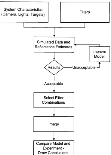
Imai (2000a).

to establish a _{relationship between digital} output and spectral reflectance. This

relationship is thenusedtomake spectral reflectance estimations ofaverificationtarget.

Once the spectral reflectance ofthe verification target is estimated, appropriate _quality

metricscanbeused and afiltercombination canbechosenforthe trichromaticcamerain

question. Figure 1.1 shows a flowchart ofthe general _process, which was used as the

System Characteristics

(Camera, Lights,

Targets)

Filters

V

Simulated

Data

and

Reflectance Estimates

i

Improve

Model

i'

Unacceptable

T

Acceptable

Select Filter

Combinations

Image

Compare Model

and

Experiment

[image:21.527.85.454.43.556.2]

-Draw Conclusions

Figure 1.1- General_process

cameratoperformspectralreflectance_estimation,beusedas part of a recommendationto

theNational

Gallery

of

Art,

Washington D.C. andTheMuseum ofModern Art in New

York

City

inthe constructionof aspectral

imaging

_system, as well as addtoandfurther

documentthe_growing

body

of spectral

imaging

research atMCSL.

Overview:

Chapters Two and Three give some background on spectral

imaging

and the

equipment used for this thesis. Chapter Two

briefly

discusses some ofthe previous

research done with regardsto spectral imaging.

Here,

the three main types of spectral

imaging

systems are discussed and some of their advantages and drawbacks are

described. Chapter Three describestheequipment usedforthis thesis. Thisincludesthe

camerasystem,

lights,

targets,

and other major aspects ofthesystem

being

evaluated.

ChaptersFourthroughSix discussthe simulations performed andhowthemodel

progresses froma simple linear model that is _only concerned with average values to a

more complex modelthatincorporatesaspects of system noise.

Chapter Seven describes the

imaging

_experiment, where filter selections made

basedontheresults ofthesimulations are usedina practical situation. Theexperimental

dataarethencompared withthesimulated

data,

and sourcesof error areidentified.

ChapterEightgives an analysis ofthree filtercombinations, which were chosen

based on simulated _performance, experimental _performance, and an example of poor

overall performance.

Finally,

ChapterNinegives a_recapofthis thesisand makes suggestionsfor future

Chapter

2

-

Spectral

Imaging

Systems

Background:

Spectral

imaging

and reproduction has become an

increasingly

important areaof

researchattheMunsell Color Science

Laboratory (MCSL)

as well asatotherinstitutions

around the world (Berns

1999;

Berns

2003;

Burns

1998;

Burns

1999;

Day

E.A.

2003;

Day

E.A.

2002;

Fairchild

2001;

Haneishi

2000;

Hardeberg 2003; Hardeberg

1999;

Imai

1998a-i;

Imai

1999;

Imai

2000a,b;

Imai

2002;

Imai

2003;

Johnson

1998;

Konig

1998;

Konig

1999;

Quan

2000;

Rosen 1999). Several different methods have been used to

perform spectral image capture and reproduction. Earlier systems at MCSL were

designed using filmasthespectraldetector (Rosen 1999). Asthe_availabilityand_quality

ofdigital camerashas

increased,

CCDcameras have become_commonlyused. Thereare

currently three methods that are _widelyused in

designing

spectral-based digital camera

systems. Theseare narrowband imagecapture with a monochromatic _sensor,wideband

imagecapture with a monochromatic sensor, and wideband imagecapture with an

off-the-shelf trichromaticdigitalcamera.Eachmethodhas itsadvantages anddrawbacks.

Narrowbandcapture:

The firstmethodinvolves theuse of a monochromaticdigital camera and narrow

band sampling. There are _many choices of

technology

available that provide the

spectrally narrowfiltrationrequired.

Typically,

aliquid crystal tunable filter

(LCTF)

is

usedas it has the advantages of

being

solid state and computercontrolled _meaningthat

experimentsthattheLCTFstillsuffersfromangular

dependencies,

butnot as severeasin

other

technologies,

suchasnormal

interference

filters. WhiletheLCTFdeliversthemost

accuracyas _many samples across thevisible spectrum are used, it is generallythemost

costly,time _consuming, andgenerates large amounts ofdata thatmust thenbemanaged

later. Figure 2.1 shows a LCTF attached to a Roper Scientific Quantix at the MCSL

[image:24.527.177.376.214.368.2]

Spectral

Imaging

laboratory.

Figure 2.1- Quantix_{camera with}LCTF_attached.

Widebandcapture:

Thesecondmethod uses a smaller set of wideband filterstocapturedigital image

data and then uses reconstruction algorithms to estimate the reflectance spectra of an

object. This approachproduces reasonable results because bothman made and natural

materials _generally have smooth spectral reflectance _shapes, thus the _{sampling interval}

canbereducedtobetweeneight andtenchannels withbroader bandpass filters whilestill

achievingaccurate results. Thishas generally beentheaccepted method ofimagecapture

as it is a good compromise between accuracy and efficiency. _{Systems using} this

as the National

Gallery

in

London,

England and the Uffizi

Gallery

in

Florence,

Italy.

These

institutions

are involved in the VASARI (Visual Arts System for

Archiving

and

Retrieval of

Images)

_program, which has successfully used a seven channel camerato

capture multi-spectral informationand _{map it}

directly

to colorimetric space. Figure 2.2

showstheVASARIsystem.

Figure2.2- The VASARI_{system(National}

Gallery,London).

Trichromaticcamerawith absorptionfilters:

The third methoduses ahigh qualitytrichromatic digital camera in conjunction

with spectral absorption filters to acquire unique spectral information. This method

enables three channels ofdata to be captured per exposure as opposed to one. This

red, green, and blue spectral sensitivities ofthe camera. Figure 2.3 shows the IBM

Pro3000systemusedin manyoftheexperimentsperformed atMCSL.

Figure 2.3

-IBM Pro3000 scanningcamera.

Conclusions:

This chapter has given a brief discussion ofthe three main technologies most

commonly used to perform spectral image capture.

Usually,

the choice of which

technology

touse willdependuponseveraldifferent

factors,

including

thepurposeofthe

images,

price, availability, and accuracy. As was mentioned in the

introduction,

this

thesis _{is mainly} concerned with the trichromatic approach and

developing

methods to

Chapter 3

-Equipment:

Purpose:

Themaingoal ofthisthesiswastoshowthatit ispossibleto selectfilters thatcan

beused with ahighresolutiontrichromaticdigital cameratoperform spectral reflectance

estimation. The

following

equipmentwas used for_{measurement, modeling, simulation,}

andfortheexperiment.

Pixel Physics TerraPixcamera system:

The TerraPix camera

by

Pixel

Physics,

shown in Figure

3.1,

uses aMegavision

T4 camera back. This back is based on the Kodak KAF-16801E CCD sensor. This

sensor providesimageswitha resolution of4096X4096pixels. The CCDuses aBayer

pattern colorfilterarray, andtherawdatamustbe interpolatedto deliverred, green, and

blue imageplanes. The cameraback was used with a Contax 645 camera

body

and an

80mm Carl Zeiss T*

Diagnon lens. The image capture software was custom made

by

Pixel Physics. Other _processing software used was created

by

Lawrence Taplin at

MCSL. For simulations, the camera's spectral sensitivities were also provided

by

Pixel

0.16

|

0.04 Q.

CO

0.02

500 550 600

Wavelength

(nm)

Figure 3.2- TerraPix_{unfiltered spectral sensitivities.}

ElinchromeScanliteDigital 1000:

Two Elinchrome ScanliteDigital 1000studio lightswere usedforthesimulations

and experiment. Chimera Pro Light diffusers were attached to the light sources to

provide

diffuse,

evenlighting. Figure3.3 shows the light sources andFigure 3.4 shows

their relative spectral powerdistribution measured with aPhoto Research Spectra Scan

PR-650 handheld spectroradiometer. At the image plane, the correlated color

temperature was measured to be _{approximately} 3,334 degrees Kelvin. The luminance

too

Figure 3.3- Scanlite_withlight diffuser.

450 500 550 600

Wavelength

(nm)

650 700

Hummeltal,

Germany)

was used in combination with the reflectance data ofthe blue

pigment target _consisting of _{phthalocyanine, ultramarine, cobalt,} and Prussian blues

mixedin differentcombinationsandconcentrationswithtitaniumwhite. TheEssertarget

was chosenbecause ofits spectralvariability. Itwas _necessaryto add the spectrafrom

pigments ofthe blues targetbecause thesepigments are

typically

found in art paintings

but are not represented on the Esser target. The Gamblin paint target was used as the

main verification target. Itwas composed of30 pigments _{commonly found in artwork,}

each mixed at two concentrations with titanium white. Both the blue pigment and

Gamblintargetwerehandpainted onto a piece of canvasboard found in_manyart stores.

Figure 3.5 showsthereflectance spectrafor allthe samples ofboth these targets. Other

targets included a Kodak

Gray

Scale as well as the GretagMacbeth ColorChecker and

ColorChecker

DC,

shown in Figure 3.6. The targets were measured _using a

GretagMacbeth ColorEye XTH handheld

integrating

sphere spectrophotometer withthe

400 450 500 550 600 650 700 750

nm

1

0.9

0.8

..0.7

o

I

0.6

0.5

"0.4

*0.3

0.2

0.1

0

;^a ML

"*""%*~ "

^"."r^rrTTz?^*.

IV

\ /

j$f

\

\

\

\Ji/j

Mivi

i^"-^->;rf^

--/*>=^^

/

/llz^^^Lv^vvz

/U/ _/^-^rfc-^ .

1 fZ *^7 yfl ^*n v

IllU- _<i Zt^ yJZ'

Wwk

i.

^^^^^^l

~

i i i

' i

400 450 500 550

nm

600 650 700 750

Figure 3.5- Reflectance_{spectra of all samples on}theEsser_andBlues_{characterizationtarget} (top)

Figure 3.6- Targetsimaged: Blue_pigments(upper

left),Macbeth Colorchecker_(center),Essertest target(upperright),Kodak

Gray

Scale_{(left/center),}halon disk_{(right/center),}MacbethCCDC

(lower_left),Gamblinpigments_{(lower right)}

Filters:

A set of105 Kodak Wratten filters were evaluated. These selective absorption

filters are used in a wide _variety oftechnical and photographic

imaging

applications.

Transmittance filters were selected because their spectral properties do not have the

angulardependencethatisfoundininterference

filters,

showntohavea significant effect

on spectral estimation and reconstruction accuracy. The nominal data used for

simulationswere provided

by

Kodakand spanthewavelength range of400-730nm.

AUnaxis Balzers IRcutofffilterwas usedtolimitthe spectrum ofinterestto the

visible region (400 - 730

nm). The transmittance data used for simulations was

measured with a Macbeth ColorEye 7000

integrating

sphere spectrophotometer in the

Processing:

All simulations and data processing were performed _using Matlab versions 5.3

and 6.5. Code for all processes are in Appendix

B,

and is adaptable to _any platform

Chapter

4

-

Filter

Selection for Spectral

Estimation using

a

Noiseless Camera Model:

Purpose:

This chapter is concerned with

describing

filter selection in a noiseless case.

First,

the

theory

of spectral reconstruction_usingmultiple camera signals and eigenvector

analysis is

described,

andthenthemethod and metrics usedtoselect an appropriate filter

arediscussed.

FilterSelectionMethod:

The first factor that was considered was the method of _{searching for filter}

combinations. Several different approaches can be used and have been discussed

(Hardeberg

2003). The first and most intuitive method was to _simply

try

to find a

combination of filters where the dominant wavelength is _equally spaced across the

spectrum of interest. While this approach worked well for monochromatic cameras

which _only consider one channel at a time and have a _{relatively flat} response when

unfiltered, it is very difficult to find a filter that will cause three channels in a

trichromatic camerato shift_{significantly}without_entirely

blocking

thesignal in anyone

channel. The second, which was first proposed

by

Maitre and expanded on

by

Hardeberg,

involves_maximizing the_{orthogonality}inthecharacteristicreflectance vector

space

(Hardeberg

2003). This method was shown to be

fast,

_{but only} considered one

channel at a time and demonstrated suboptimal results. The final method was an

exhaustive search which considers all possible combinationsoffilters inquestion. Dueto

thecomplex natureofthe taskat

hand,

thismethodwas chosenbecause it_will,in theory,

findtheoptimal results fromallcombinations. Caremustbetakenwiththisapproach as

the number of computations can _{easily become very} large given that the number of

evaluationsis determined

by

Eq.4.1

g=

I*

N!

(4.1)

K!(N-K)!

where_{g is} thenumber of_{combinations, N}isthe total number offilters inthe set,andK

arethenumber offilters

being

combined

(Hardeberg

2003).

Spectral Reconstruction Theory:

Reflectance spectra of objects canbeestimated

by

_usinga priorispectral analysis

withdirectmeasurement and

imaging

of color patchestoestablish a_relationshipbetween

cameradigitalcountsandspectralreflectancefactor (Imai 2000a).

The spectral reflectances ofa set of samples from a characterization target are

measured and (n x _q) reflectance matrix R is

formed,

where n is the number of

wavelength measurements and _q is the number ofmeasured samples.

Using

principal

component _analysis, <r eigenvectors

{ei...ef}

and the associated eigenvalues are

calculated and arranged in

descending

order. The cumulative contributionindex

(CCI),

v thatdescribes the amount of variance explained

by

the first i eigenvalues isgiven

by

where aisthevectorof eigenvalues. _{The CCI is generally}usedto

help

selectthenumber

of eigenvectors to beused inthe spectralreflectance reconstruction inconjunction with

othercolorimetric and spectral metrics(Imai 2000a).

Theestimatedspectralreflectanceis defined

by

Eq.4.3

R=E,a,

(4.3)

A

where

E,=[ei...e,],

the coefficients _a(=[ai...a,] , and R represents the estimated

reflectances.

A camera system gives (b x _q) digital _counts,

D,

where b is the number of

channelsand _{q is}thenumber of samples or pixels_{corresponding}tovarious samples. In

general,thenumber of channels

being

used shouldbeequaltoor greaterthan thenumber

of eigenvectors

(Imai, 2000a)

used in the estimation. The _relationship between the

eigenvalues

a,-ofthe targetanddigitalcounts ofthecharacterizationtarget

Dc

isgiven

by

Eq. 4.4:

Te=a,/wn>(Dc)

(4.4)

where_pinvQ denotes the Matlab function which performs the equivalent of a

pseudo-A

inverse calculation. The matrix

Te

can then be used to estimate eigenvalues a, from

digitalcounts of a verificationtarget

Dv

as shownin Eq. 4.5:

a,=TeD

(4.5)

Finally,

reflectance oftheverificationtarget

Rv

is estimated

by

_{substituting Eq. 4.5 into}

Rv=E/reDv

(4.6)

Acamera withlinearphotometric responsecanbemodeled_usingEq.

4.7,

andthe

simulated digital counts can then be used to establish the _{relationship between} camera

digitalcountsandobjectspectralreflectance:

dk=XpWrWS//(A)f(/l)AJl

(4.7)

X

where _{p(A.) is} the source relative spectral power

distribution,

_r(k) is the spectral

reflectance ofthe _{object, s^QC)} is the appropriate camera channel _sensitivity,

f(A.)

is the

filter

being

_used,and u=

R,

G,

orB.

Experimental:

An experiment was designed to

identify

a subset offilters from a set of_readily

available filterstobeused forspectral reflectance estimation with atrichromaticcamera.

The simulation experiment involved _calculating the TerraPix camera's filtered camera

signal when

imaging

a characterization and verification_{target, estimating}the reflectance

ofthesamples,andthen_makingafilterselectionthatprovidesgoodperformance.

The eigenvectors and eigenvalues ofthe combinationEsserandbluestargetwere

calculated_using eigenvector analysis andthe knownreflectance spectra ofthepatches.

The eigenvectors were thenranked from most significantto leastsignificant and a CCI

was calculated. Thenumberof eigenvectors selectedis typicallyacompromisebetween

eigenvectors calculated for the CIE 1931 standard observer and illuminant

D65,

for

which all subsequent calculations willbemadeunless notedotherwise,showingthat99%

of the variance in the data can be described with six _{eigenvectors, the} CCI stops

increasing

significantlyat six _{eigenvectors,} andthe metrics _stop

decreasing

_{significantly}

Table 4.1-Cumulative

contributionindexand metricsfor the 1931standard observer andilluminant

#of

Eigenvectors CCI

Average % RMS spectral error

Average CIEDE2000

Average Metameric IndexD65->A

Average Metameric IndexA->D65

1 0.63 18.2 44.71 4.70 5.78

2 0.86 6.7 18.02 1.34 2.08

3 0.97 3.3 4.18 1.27 1.49

4 0.98 2.4 1.29 1.25 1.43

5 0.99 1.7 0.97 0.29 0.30

6 1.00 1.3 0.52 0.20 0.23

7 1.00 1.1 0.27 0.15 0.15

8 1.00 0.9 0.18 0.11 0.13

9 1.00 0.8 0.16 0.04 0.04

10 1.00 0.6 0.14 0.02 0.02

11 1.00 0.5 0.15 0.02 0.03

12 1.00 0.3 0.06 0.02 0.03

Based on this

information,

data from previous experiments _analyzing color

difference and spectral RMS error _showing that six channels is _sufficiently accurate

(Imai, 2000a),

and information obtained from the

CCI,

six channels obtained

by

combining the three channels from each image were used for this and the

following

experiments.

Having

determined an appropriate number of eigenvectors to use in the

reconstruction,allpossiblecombinations ofdata fromtwofilters simulated with equation

4.6were evaluated. Thedataweresimulatedfor digitalcounts generatedfroma response

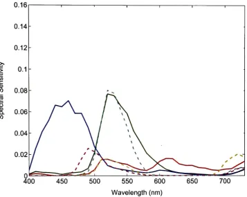
integrated over the 400

-730 nm range. This range was chosen _{partly because many}

show_respectivelythe spectraltransmittance propertiesandthe_resulting camera spectral

sensitivitiesoftheIRcutofffilter.

400 450 500 550 600

Wavelength

(nm)

650 700

0.16

0.14

0.12 >>

o

c

9> o m 111 E

C

CO

O

^ _0.08

>

'in

c

CD

CO

TO

0.04 o

CO Q.

CO

0.06

0.02

400 450 500 550 600 650 700

Wavelength

(nm)

Figure 4.2- TerraPix_{spectral sensitivities with}UV/IR_{cutoff applied.}

Using

the 105 Kodak Wratten filters and the unfiltered _case, a total of 106

separate sets of simulated digital counts were created and takenin combinations oftwo

givingatotalof5565unique combinations. Thesecombinations were usedtoreconstruct

the reflectance spectra of the Gamblin verification target. The mean and maximum

CIEDE2000 for illuminant D65 and the2 degree observer was calculated andthe RMS

spectral error overtherange of400- 730

nmacross all thepatches was thencalculated

ResultsandDiscussion:

Figures 4.3and4.4showthedistributionofthefiltercombinations with respectto

the average CIEDE2000 and RMS spectral error. It not _only shows that a large

percentage ofthe combinations perform _{equally well,} but the range ofthe metrics are

relatively small for those that doperform well. This lends to a degree of

difficulty

in

selecting the best combinations from just the mean and maximum metric measures.

Another method needed to be devised in order to eliminate combinations that were

unlikely to perform well and to reduce the number of filter combinations to a more

comprehensible level. The

following

method was used to sort the filters and make

eliminations.

1800

10 15 20

Average %RMS Spectral Error

25

10 15

Average CIEDE2000

20 25

Figure 4.4-Histogram_ofthe

averageCIEDE2000calculatedfromallfiltercombinations.

The metrics'

correlation coefficients were calculated and thepairthat correlated

best was plotted against each other. Table 4.2 shows the calculated correlation

coefficients.

Table 4.2- Metric_{correlation coefficients.}

Average

spectralRMS

Maximum

spectralRMS

Average

CIEDE2000

Maximum CIEDE2000

Average

spectralRMS

1.0000 .9013 .9019 .7780

Maximum

spectralRMS

0.9013 1.0000 .7810 .7807

It shows that the average CIEDE2000 and RMS spectral error correlate best and were

used as a first criteria. The maximum CIEDE2000 and RMS spectral error were then

used as a second selection criteria. The combinations were then sorted

by

_selecting

threshold levels ontheplot oftheaverage_{metrics, observing}wherethosepoints plotted

on the maximum metric plot and then _selecting thresholds on the maximum and

observingwherethenew_{group falls}ontheaverageplot. Thisprocesswas repeated until

a reasonable number was found. Figures4.5 and4.6 showthemetricplots andTable4.3

shows the thresholds and the_resulting number offilter combinations after each level of

selection. In Figures 4.5 and

4.6,

the bluerepresentstheentire set, the green represents

membersoftheset afterthefirst_sort, andthered represents members oftheset afterthe

25

20

15

o o o CN

LU Q UJ O w at

3

10 15

Average% Spectral RMS

20 25

Figure 4.5- AverageCIEDE2000_{vs. average.RMSspectral error plot usedto}

aid_{in selecting}

120

100

o o o CN 111 Q LU

o x co

20 30 40 50 60

Maximum% Spectral RMS

70 80

Figure 4.6-Maximum CIEDE2000

vs. maximumRMSspectral error plot used_{in selecting}threshold

sortingcriteria,with_{blue representing}theentireset,green_representingthefirstsort,and red

representingthesecond.

Table 4.3

-Sorting

Criteriaand_resultingnumbers of combinations.

Selection Criteria

Resulting

NumberofFilterCombinations

Average CIEDE2000<

1.5,

_AverageRMS<

2.5%

1351

MaximumCIEDE2000<

4,

Maximum

AverageRMS<6%

635

Average CIEDE2000<_.6,AverageRMS<

2%

71

Once the number of selections reached a reasonable _number, the filter

combinations were then eliminated

by

_calculating the area of the filtered camera

sensitivities for each curve. This would eliminate curves where the signal would be

signals were greater than 2.5 reduced the list to eight combinations whose metrics are

shownintable4.4andintegratedcamera signalsare shownintable4.5.

Table 4.4- Metrics_ofthe

topeightfiltercombinations_{resulting from}thenoiseless simulation.

Filter 1 Filter 2

Average % Spectral

RMS

Maximum % Spectral

RMS

Average CIEDE2000

Maximum CIEDE2000

WR-40 LIGHT GREEN WR-78A BLUISH 1.9 5.0 0.57 2.91

WR-40 LIGHT GREEN WR-80B BLUE 1.9 4.9 0.58 3.06

WR-66 VERY LT GREEN WR-78B BLUISH 1.9 4.5 0.51 2.79

WR-40 LIGHT GREEN WR-80A BLUE 1.9 4.9 0.59 3.12

WR-66 VERY LT GREEN WR-80C BLUE 1.9 4.6 0.54 3.05

WR-66VERYLT GREEN WR-78A BLUISH 1.9 4.7 0.58 3.30

WR-81 YELLOWISH NF 2.0 5.5 0.52 1.73

WR-3 LIGHT YELLOW WR-82C BLUISH 2.0 5.0 0.49 2.30

Table 4.5- Integrated_{camera signals ofthe}

topeightfiltersresu

Iting

fromthenoiselesssimulation.

Integrated Camera Sgnal

Filter1 Filter 2 R1 G1 B1 R2 G2 B2

WR-40 LIGHT GREEN WR-78A BLUISH 3.18 5.24 2.65 3.86 4.16 5.00

WR-40LIGHTGREEN WR-80BBLUE 3.18 5.24 2.65 4.31 4.38 5.62

WR-66 VERY LT GREENWR-78BBLUISH 5.95 8.26 4.79 7.15 6.90 6.86

WR-40 LIGHT GREEN WR-80A BLUE 3.18 5.24 2.65 3.39 3.79 5.33

WR-66 VERYLT GREENWR-80C BLUE 5.95 8.26 4.79 6.42 6.14 6.61

WR-66 VERYLT GREEN WR-78A BLUISH 5.95 8.26 4.79 3.86 4.16 5.00

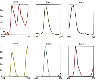
WR-81 YELLOWISH NF 15.89 12.85 9.95 17.83 14.75 11.73

WR-3LIGHTYELLOW WR-82C BLUISH 16.08 13.07 6.68 8.51 8.31 7.68

Final selections could _{only be} made after _evaluating curve shapes and the

resulting camera sensitivities as well as the different metrics measured for this case.

yield a_{comparatively}goodRMS spectralerror and_verygood colorimetric_results,yetthe

resultingcamera sensitivities are almostequivalent,as showninFigure4.9.

Findmetricsthatcorrelate

best,

plottwo scatter plots of

correlating metrics

Selectgroups with threshold

levelson one_plot, plotthe

groups onthesecondplot

NO- Alternate

plots

that threshold isselected from

and plotted on

Find area of

integratedsignals

- _eliminatefilters

with lowsignal

Evaluate remaining

curves andcamera

sensitivities

-make

selections

Figure4.7- Flowchart

o CO

Li-Cl) o

C CO

*s

E

CO c

CO

100 450 500 550 600 650

Wavelength

(nm)

Figure 4.8- Wratten 81_yellowishfilter_{spectraltransmittance.}

c

o

ui

E

+-< c CO 3

0.16

0.14

0.12

2-

_0.08

0.06 a)

co

I

0.04 o

CD Q.

CO

0.02

100 450 500 550 600

Wavelength

(nm)

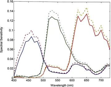
Figure4.9- Filtered_{and unfiltered}TerraPix_{spectral sensitivities after}

usingtheWratten81.

This combination's performance can be further explained

by

looking

at the

transformation matrix that was used to convert the digital counts of an image to the

coefficientstobeused withtheeigenvectorstoreconstructthespectral reflectance. Table

Table 4.6- Matrix for Wratten 81

andNo FilterCombination.

Camera Channel

R1 R2 G1 G2 B1 B2

Coefficients

1 -12.01 12.21 143.65 -123.11 10.81 -10.28

2 129.64 -116.10 -115.57 102.58 -246.16 220.30

3 163.70 -145.28 132.79 -118.82 -215.57 188.43

4 -398.18 358.61 400.59 -349.84 -381.71 322.87

5 -34.94 34.96 -873.72 753.15 400.66 -337.30

6 180.80 -156.08 -39.73 37.43 -558.21 464.52

Thismatrix_{is showing}thecontribution of each channeltoa particular coefficient. These

matrices work ina noiseless case because it is built offthe average simulated values of

the Esser and blues target. In reality, a _group of pixels associated with a particular

reflectance spectrum willhave variance. This particular matrix would then_amplify the

variance andintroduceanincreasedamount of errorintothesystem. For example,the4

coefficient shows that the contributions of the first two channels are multiplied

by

approximately -398.18 and 358.61. If the digital counts from a particular patch

corresponding to these channels varied even

by

a _very small amount, the difference

would become greatly amplified. This example can be looked at as an example where

there is a mathematical solutionto the problem with no physical meaning. Figure 4.10

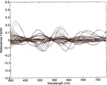
shows plots ofthe transformation matrix coefficients as a function ofwavelength. It

appearsthe transformis_verysymmetric aboutthex-axis andiscomposed of a number of

400

100 450 500 550 600

Wavelength

(nm)

650 700

Figure 4.10- Transformation_matrix

resulting fromtheWratten 81and unfiltered combination. Notethe_{extremely large}scale.

A much better choice _{resulting from} this filter selection process would be the

combination ofthe Wratten 40 and Wratten 80A filters. Figures 4.11 and 4.12 show

o

"5

co u.

(D o

c

co

E <n c

co

1

0.9

0.8

0.7

0.6

0.5

0.4

0.3

0.2

0.1

I

WR-40 WR-80A

00 450 500 550 600 650 700

Wavelength

(nm)

0.16

400 450 500 550 600

Wavelength

(nm)

650 700

Figure 4.12- TerraPixCamera_{sensitivities after}filtration_withtheWratten 40_and80A filters.

For comparison, the transformation matrix to convert camera signals to eigenvector

coefficientsis shownintable4.7.

Table 4.7- Transformation_matrixfor Wratten 40_and80A filters.

Camera Channel

R1 R2 G1 G2 B1 B2

Coefficients

1 1.4936 12.828 -7.4842 14.802 -0.9164 -3.4039

2 0.089341 -6.4197 5.3418 0.74343 -6.2315 29.036

3 5.0673 5.3384 9.4926 -34.009 -15.772 21.536

4 -4.4362 3.5821 -12.897 18.277 -12.911 12.465

5 -22.791 22.761 24.121 -44.337 35.162 -13.831

6 4.4082 5.8228 26.445 -31.974 -50.31 19.202

Thevaluesinthetransformationmatrixaremuch smaller_suggestingamore stable matrix

amplified with this transformation matrix and would be more

likely

to perform well in

actual

imaging.

Figure 4.13 shows the transformation matrix coefficients. Notice the

scale on the _y axis is smaller,

indicating

_{that a difference in pixel values will be less}

amplified.

Theoretically,

_{this transformshouldbe}

morerobusttonoise.

500 550 600

Wavelength

(nm)

650 700

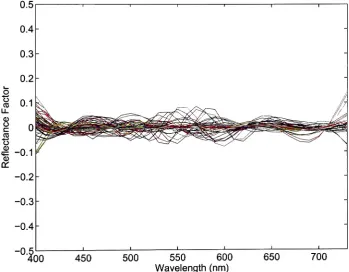
Figure 4.13- Transformation_{matrixcoefficients}

resulting fromtheWratten 40and80A combination. _{The y}scaleismuch smallerthanin figure_{4.10,suggesting less sensitivity}tonoise.

Conclusions:

Thenoiseless simulation canbeused as a preselection methodfor filterselection

taken into consideration.

Otherwise,

as shown withtheexample oftheWratten 2C and

nofiltercombination, erroneousselectionscanbemade. In any filterselection_case,it is

Chapter

5

-Modeling

the

Camera

Noise for Simulation:

Purpose:

While a camera with linear photometric response can be modeled as shown in

equation

4.6,

_{it is only} a measure ofthe average signal from the camera and does not

includenoise. A lackofnoise ona perpixelbasiscanleadtofilterselectionsthatdonot

make intuitive_sense, as wasshowninthenoiseless case. Thischapterdescribes howthe

noise variance in the TerraPix camera was modeled and applied to the basic camera

equationtosimulatethecamera response

including

noise.

The results ofthe noiseless simulation returned several filter combinations that

perform_similarly and made it difficultto_classifythe filters intermsof performance. It

was also shownthatsome ofthe filtercombinations thatdemonstratedgood performance

did not make intuitive sense. Filters combinations that fell into this _category were

usuallycombinations offiltersthatwere_verysimilarintheir transmittancepropertiesand

did relatively littletoalterthecamera signalsfromeach other. Itwasdeterminedthat the

addition of noise and a simulation of multiple pixels withtheappropriate noise properties

could be used to create more realistic reflectance estimates and give more physical

meaning to the results of_simulating the camera's response to different filters foruse in

spectral reflectance estimation.

Also,

the simulationof_manypixels would allowtheuse

of adirect pseudo-inverse transformas opposed to the eigenvector analysis used inthe

Noise Sources:

Noiseis defined to_{be any}unwanted signalthatcontains no

information,

whichis

addedto the imageroutput (Eastman Kodak

Company

1994). Thefirstmajor source of

noise comesfromtheCCD imager itself. A CCDcamerahasseveral sources ofinherent

noise that are alldependent onfactors such as

time,

_signal, and temperature. The main

sources oftemporalnoiseinaCCD imager include dark_current,photon shotnoise, reset

transistor noise, CCD clocking noise, and noise from the output amplifier (Eastman

Kodak

Company

1994). Dark current noise is dependent onthe _operating temperature

and the integration time. The dark current noise also varies across the pixels ofthe

imager,

leaving

afixedpatternnoise. The darknoise canbe dealtwith

by

taking

adark

imageorthe average of severaldarkimages attheappropriateintegrationtimeand_using

the average pixel referenced data as the zero level for each pixel (Eastman Kodak

Company

1994). Thereset transistornoise and output amplifier noise isgenerally dealt

with

by

_using different methodsof_samplingthe signal, butis beyondthe scope ofthis

research.

Finally,

thephoton shot noise cannotbeeliminated,butcan alsobereduced

by

taking

severalimagesand_averagingthedata.

The second source of noise comes from the scene illumination. While _every

attempt is made to create uniform illumination across the scene, in practice there is

always a certainamountofvariationimposed

by

theunevennessin

lighting

and optics of

the system. Thisnoiseis dealtwith

by

taking

areferenceimageof a uniform

target,

such

as an even _graysurface ofknown reflectance and_using it to flat fieldthe

image,

which

canbemathematicallydescribedinEq. 5.1.

D-D Dc=("r

\T

)*(PEr.y

-D-.*)

<51)

where

Dc

isthecorrected

data,

Dr

_{is theraw}

data,

D^y

is the_graycard,

Ddark

isthedark

exposure and

(D^

-Ddark)

denotes

theaverage_grayvalue overthe area oftheuniform

gray card. This is a _very common method of_reducing the variation in output signal

across ascene andis easily done inacontrolled environment.

Experimental:

Equation 4.6 gives the noiseless camera model in terms of a _relative, average

signal. Theequationisnow changedtothe

following

form:

d

=_{ptJ]pWr(X)sliWfWAA4n}

(5.2)

x

wheretistheintegration

time,

pisaconstantthatconvertstheintegratedsignaltodigital

counts and n is the noise associated with the signal. In the noiseless _case, the_p and t

termcanbe

ignored,

as

they

are constantsthatare dealtwith inthe transformgenerated

by

theeigenvector analysis. It isnow_necessarytoincludethesetermsbecausethenoise

isasignaldependent factorthatisinturndependentuponintegrationtime.

The noise characteristics of the camera were determined from images taken

during

an

imaging

sessionattheNational

Gallery

of

Art,

WashingtonD.C. Atthe

time,

theIRcutofffilterwas supplied

by

Pixel Physicsand cutstransmittance_{approximately}at

700 nm. Future simulations withthe model willbe based onthecamera_sensitivity and

the Unaxis Balzers UV/IR

blocking

filter that extends transmittance into the near IR

which 240 patches each of2883 (31 x 31 x

3)

pixels were sampled. These patches

consisted of236

individual

sample areas

measuring

1.3 x 1.3 cmandfoursamplesfrom

the

large

central square. _{The first step} wasto

determine

the variance characteristics of

the camera as a

function

of mean signal level. This was done

by

taking

the raw,

unfiltered

images

and_processingthemwiththesoftware provided

by

Pixel Physics_using

amodethatreturnedthedatascaledto 16 bitswithno correctionsapplied. Themean and

varianceoftheindividualpatcheswerethenplotted andfit_usingthe_robustfitQ algorit