An optimization framework for solving capacitated multi-level lot-sizing problems with backlogging

manuscript (Please, provide the mansucript number!)

An Optimization Framework for Solving Capacitated

Multi-level Lot-sizing Problems with Backlogging

Tao Wu†, Leyuan Shi†, Joseph Geunes‡, Kerem Akartunalı∗

†

Department of Industrial and Systems Engineering, University of Wisconsin-Madison, Madison, WI 53706

‡

Department of Industrial and Systems Engineering, University of Florida, Gainesville, FL 32611

∗

Dept. of Management Science, University of Strathclyde, Glasgow G1 1QE, UK

This paper proposes two new mixed integer programming models for capacitated multi-level lot-sizing prob-lems with backlogging, whose linear programming relaxations provide good lower bounds on the optimal solution value. We show that both of these strong formulations yield the same lower bounds. In addition to these theoretical results, we propose a new, effective optimization framework that achieves high quality solutions in reasonable computational time. Computational results show that the proposed optimization framework is superior to other well-known approaches on several important performance dimensions.

Key words: Capacitated, Multi-level, Lot-sizing, Backlogging, Lower and Upper Bound Guided Nested Partitions

1.

Introduction

This paper considers the Multi-Level Capacitated Lot-Sizing problem with Backlogging (ML-CLSB), a class

of problems often faced in practical production planning settings. The goal of this problem is to schedule

pro-duction at each level of a complex bill-of-materials structure over a finite horizon, while minimizing total cost

and ultimately meeting all customer demands by the end of the horizon. The total relevant costs include setup

costs, inventory holding costs, and backlogging costs. The output of this model consists of the setup periods

and the time-phased production, inventory, and backlog quantities at each stage of the bill-of-materials over

the planning horizon. Effective solution of this problem is one of the most important determinants of cost

performance in any dependent-demand production and inventory control system, which includes the

well-known material requirements planning systems prevalent in manufacturing practice. Research on models and

solution methods that facilitate more efficient solution of problems in this class thus has the potential to

provide tangible benefits to practitioners in the form of lower total production-related costs.

Past literature on the ML-CLSB is reasonably sparse due to the problem’s complexity. Most of the past

research considered simpler problems, such as the uncapacitated and single-level lot-sizing problems with

backlogging. For instance, Zangwill (1969) investigated single level lot-sizing problems with backlogging.

Pochet and Wolsey (1988) studied extended reformulations of uncapacitated lot-sizing problems with

back-logging and explored their relationships. Federgruen and Tzur (1993) developed an O(n log n) dynamic

programming algorithm for a standardn-period single-level lot-sizing problem with backlogging. Millar and

Yang (1994) proposed two Lagrangian decomposition and Lagrangian relaxation algorithms for solving the

capacitated single level multi-item lot-sizing problem with backlogging. Agra and Constantino (1999)

exam-ined the uncapacitated single item lot-sizing problem with backlogging and start-up costs, when

Wagner-Whitin costs are assumed. Cheng et al. (2001) formulated single-level lot-sizing problems with provisions

for backorders using a fixed-charge transportation model and proposed a heuristic solution method. Ganas

and Papachristos (2005) proposed a polynomial-time algorithm for the single-item lot-sizing problem with

backlogging. Song and Chan (2005) proposed a dynamic programming algorithm for solving a single-item

lot-sizing problem with backlogging on a single machine at a finite production rate. Mathieu (2006) proposed

two extended linear programming (LP) reformulations of single-item lot-sizing problems with backlogging

and constant capacities. In a recent study, K¨u¸c¨ukyavuz and Pochet (2009) provided the full description of

the convex hull for the single-level uncapacitated problem with backlogging. We refer the interested reader

to Pochet and Wolsey (2006) for a detailed general review of different lot-sizing problems. We note that the

termbacklog is used interchangeably withbackorder in the lot-sizing literature, referring to any demand that

is not satisfied on time but in a later time period, no matter what type of manufacturing environment. In

our context, we consider a model that is flexible enough to apply to both MTO (Make-To-Order) and MTS

(Make-To-Stock) environments when production is planned based on fixed demands or forecasts.

The past research has also considered other classes of lot sizing problems. For example, Thizy and van

Wassenhove (1985) designed a Lagrangian relaxation (LR) approach, in which capacity constraints are

relaxed, in an attempt to decompose the problem into N uncapacitated single item lot-sizing

subprob-lems, solvable by the Wagner-Whitin algorithm. Trigeiro (1987) developed a similar approach for solving

the deterministic, multi-item, single-operation lot-sizing problem. Trigeiro et al. (1989) also proposed LR

based methods for large-scale lot-sizing problems. Kuik and Salomon (1990) evaluated a simulated annealing

heuristic for solving multi-level lot-sizing problem. Pochet and Wolsey (1991) applied strong cutting planes

to solve two classes of multi-item lot-sizing problems, a class of single-stage problems involving joint machine

capacity constraints and/or start up costs and a class of multistage problems with general product structure.

Salomon (1991) developed a tabu search procedure where the solution set is searched quickly in a greedy

fashion. Kuik et al. (1993) proposed an LP-based heuristic, and compared the performance of the heuristic

with the performance of approaches based on simulated annealing and tabu search techniques. To solve the

capacitated single-item lot-sizing problem with setup and reservation costs (a separate reservation cost is

incurred for keeping the resource on, whether or not it is used for production), Hindi (1995) developed a

tabu search scheme that was shown to be capable of reaching an optimal solution for a large number of

varied problem instances tested. Also, Hindi (1996) developed a tabu search procedure for solving the

capac-itated single-level multi-item lot-sizing problem using a combination of other techniques, such as column

generation. ¨Ozdamar and Bozyel (2000) proposed a heuristic that combines genetic algorithms and

simu-lated annealing to solve the capacitated multi-item lot-sizing problem. Barbarosoglu and ¨Ozdamar (2000)

described an analysis of different neighborhood transition schemes and their effects on the performance of

a general purpose simulated annealing procedure for solving the capacitated dynamic multi-level lot-sizing

problem with general product structures. Miller et al. (2003a,b) studied the polyhedral structure of an MIP

model that occurs as a relaxation of a number of structured MIP problems (e.g., capacitated lot-sizing

problems with setup times and fixed-charge network flow problems), characterized the extreme points of

the convex hull, and defined cover inequalities and reverse cover inequalities for lot-sizing problems with

multiple products, multiple resources, multiple periods, setup times, and setup costs. Tang (2004) provided

a brief presentation of simulated annealing techniques and their applications in lot-sizing problems. Simpson

and Erenguc (2005) developed a neighborhood search heuristic method for capacitated multi-stage

prob-lems. Karimi et al. (2006) proposed a tabu search heuristic for the capacitated lot-sizing problem with setup

carryover. Almada-Lobo and James (2010) proposed a meta-heuristic that incorporates a tabu search and

a neighborhood search meta-heuristic to solve the capacitated multi-item lot-sizing and scheduling problem

with sequence-dependent setup times and costs.

Akartunalı and Miller (2009) provided one of the few past works that directly considers the ML-CLSB.

They generalized the traditional inventory and lot-sizing model originally proposed by Billington et al. (1983),

and they added classical lot-sizing (`, S) inequalities, which are quite effective in improving LP relaxation

lower bounds. They also proposed a heuristic framework for solving problems within this class. Their research

was significant in advancing the techniques for solving the ML-CLSB; however, computational results of their

framework leave significant room for improvement. In order to further advance the techniques available for

solving such problems, we propose two new mixed integer programming (MIP) models that are able to yield

strong LP relaxation lower bounds. A new optimization framework is also proposed for this problem class,

which can significantly improve solution quality when compared with the prior heuristic methods.

We refer to our new optimization framework as LugNP−Lower and upper bound guided Nested Partitions.

LugNP is a method based on partitioning and sampling, which focuses computational effort on the most

promising region of the solution space. The basic premise of the framework is that an efficient partitioning

and sampling strategy can be achieved by combining domain knowledge from exact and heuristic methods

to leverage the strengths of both of these approaches. In this framework, exact methods are used to generate

lower bound solutions, while heuristic methods are used to achieve feasible upper bound solutions. The

optimization framework effectively utilizes both lower and upper bound solutions, and then provides an

efficient partitioning and sampling strategy. The search is largely restricted to the most promising region(s)

where good solutions are likely clustered.

LugNP is an extended version of the nested partitions (NP) approach proposed by Shi and ´Olafsson (2000,

2007). NP has been efficiently applied to a wide range of MIP problems, such as the traveling salesman

problem (Shi et al. 1999), the product design problem (Shi et al. 2001), and the local pickup and delivery

problem (Pi et al. 2008). However, the generic NP method is not able to partition promising regions in

the case of the complex ML-CLSB sampling problems. LugNP has similarities with the hybrid NP and

mathematical programming (HNP-MP) approach proposed previously (Wu et al. 2010). LugNP is superior

to HNP-MP in that (i) its method for identifying promising regions can cluster good solutions together, (ii)

its partitioning and sampling approach can lead to higher-quality sampled problems or subproblems, and

(iii) it continuously refines upper bound solutions, which helps improve the efficiency of partitioning and

sampling.

In order to convey the advantages of the proposed approach, it is necessary to explain its similarities

to and differences from the classical branch-and-bound approach. The branch-and-bound method creates

fathomed or eliminated (i.e., when their lower bounds are larger than the current best upper bound). When

the number of branches is particularly large, it is impossible to search all branches because of computational

resource constraints. In LugNP, a subset of integer variables is fixed using branches as well. However, some

branches are deemed to fall within a so-called promising region, while other parts are considered to be in the

surrounding region. To avoid the disadvantages associated with the standard branch-and-bound approach,

LugNP does not search all branches with equal focus. Instead, using domain knowledge provided by lower and

upper bound solution values, it effectively places greater effort on promising branches that can possibly lead

to near-optimal solutions. Both LugNP and NP are similar to beam search methods in placing greater focus

on promising regions (Pinedo 2008). However, LugNP is significantly different from beam search methods in

the way it identifies promising regions, the way it partitions promising regions into several subregions, and

in obtaining good samples of subproblems, in addition to its ability to perform backtracking.

The remainder of this paper is organized in five sections. Section 2 proposes two MIP formulations, which

are capable of generating tight lower bounds. This section also theoretically demonstrates the relationship

between these two formulations. Section 3 first details our optimization framework as applied to generic

mixed integer programs, and then discusses its application to the ML-CLSB. Section 4 discusses the results of

computational experiments conducted on a number of previously published data sets via a comparison with

other state-of-the-art techniques. Finally, Section 5 concludes and suggests directions for future research.

2.

Problem Formulations

We make the following assumptions in defining and formulating the ML-CLSB. First, we assume that setup

times and costs are non-sequence dependent, setup carryover between periods is not permitted, and all initial

inventories are zero. Second, all production costs are assumed to be linear in production output and do not

vary over time; hence, they can be dropped from the model for simplicity. Setup and holding costs also are

assumed not to vary over time. Furthermore, end items are assumed to have no successors, and only end

items have external demands and backlogging costs. Finally, we assume zero lead times and no lost sales.

It is important to note that all these assumptions (except setup carryover) are made for ease of exposition

only and without loss of generality, i.e., the theoretical results remain valid even when they are removed. See

Ozt¨urk and Ornek (2010) for the lot-sizing problem with setup carryover as well as with external demands

for component items.

To present the problem formulations, we define the following notation:

Indices and index sets:

T number of time periods in the planning horizon. M number of production resources or machines. I number of items (subassemblies and/or end items). endp set of end items.

i, j item indices,i, j∈[1, I].

endpi set of end items that utilize subassembly itemi. q, p, t, `time period indices,q, p, t, `∈ {1, . . . , T}.

m machine index,m= 1, . . . , M.

Parameters:

sci setup cost for producing a lot of itemi.

bci backlogging cost for one unit of itemifor one period.

hci inventory holding cost for one unit of itemiremaining at the end of a period.

eci echelon inventory holding cost for one unit of itemiremaining at the end of a period. stim setup time required for producing itemion machinem.

aim production time required to produce one unit of itemion machine m. gdit gross demand for itemiin periodt.

gditp total gross demand for itemifrom periodtto periodp. edit echelon demand for itemi in periodt.

editp total echelon demand for itemifrom periodtto periodp.

rij number of units of itemineeded to produce one unit of itemj, where item j is one of the successors of itemi, but not necessarily an immediate successor.

Cmt available capacity of machinemin periodt.

Variables:

xit number of units of itemi produced in periodt. sit inventory of itemiat the end of periodt.

eit echelon inventory of itemiat the end of periodt. bit backlogging level for itemiin periodt.

yit binary setup decision variables, (yit = 1 if production is setup for itemiin periodtand 0 otherwise). uitp number of units of itemi produced in periodtto satisfy demand in period p.

witp percentage of itemiproduction in periodt used to satisfy the accumulated demand for itemifrom periodtto periodp.

2.1.

Inventory and Lot-sizing Formulation

The inventory and lot-sizing formulation for lot-sizing problems was originally proposed by Billington et al.

(1983), and was presented by Akartunalı and Miller (2009) for the ML-CLSB. In this paper, we refer to this

formulation as the inventory and lot sizing (ILS) formulation, which is written as follows.

ILS:

min I

X

i=1

T

X

t=1

sci·yit+ I

X

i=1

T

X

t=1

hci·sit+

X

i∈endp T

X

t=1

bci·bit (1)

Subject to:

xit+si,t−1+bit−bi,t−1=gdit+sit ∀i∈endp, t∈[1, T]. (2)

xit+si,t−1=gdit+

X

j∈ηi

rij·xjt+sit ∀i∈[1, I]\endp, t∈[1, T]. (3)

I

X

i=1

aim·xit+ I

X

i=1

stim·yit≤Cmt ∀m∈[1, M], t∈[1, T]. (4)

xit≤min

(

Cmt−stim aim

, X

j∈endp_i

rij·gdj1T

)

·yit ∀i∈[1, I], t∈[1, T]. (5)

si0= 0, sit≥0, bit≥0, biT= 0, xit≥0, yit∈ {0,1} ∀i∈[1, I], t∈[1, T]. (6)

In this formulation, the objective function minimizes total setup, backlogging, and holding costs over the

items, respectively, where the bill-of-materials (BOM) structure dictates the relationships among different

levels of items via the definition of immediate successor and predecessor sets. Constraints (4) enforce obeying

capacity restrictions. Constraint set (5) ensures that no production occurs for itemiin period t unless the

corresponding binary setup variable,yit, takes a value of 1, in which case the amount of production is limited

by a large value depending on the minimum of production time capacity and total demand. Constraints (6)

enforce the binary and nonnegativity requirements for variables. In this constraint set,biT= 0 indicates that

no backlogging is allowed in the final period. However, a minor change can be applied here to allow such

backlogging by requiringbiT≥0.

2.2.

Echelon Inventory and Lot-sizing Formulation

Akartunalı and Miller (2009) presented an alternative formulation for this problem. In this formulation,

three new sets of echelon variables and parameters,edit,ecit, andeit are introduced, whereedit are echelon

demands,eci are echelon inventory holding cost coefficients, andeit are echelon stock variables for alliand

t. The relationships between these echelon variables and parameters and their original counterparts can be

defined as follows.

edit=gdit, eci=hci, eit=sit ∀i∈endp, t∈[1, T].

edit=gdit+

X

j∈ηi

rij·edjt ∀i∈[1, I]\endp, t∈[1, T].

eci=hci−

X

i∈η_j

rji·hcj ∀i∈[1, I]\endp.

eit=sit+

X

j∈ηi

rij·ejt ∀i∈[1, I]\endp, t∈[1, T].

Using these relationships, the alterative formulation, referred to as the echelon inventory and lot-sizing

(EILS) model formulation, can be written as follows.

EILS:

min I

X

i=1

T

X

t=1

sci·yit+ I

X

i=1

T

X

t=1

eci·eit+

X

i∈endp T

X

t=1

bci·bit (7)

Subject to:

xit+ei,t−1+bit−bi,t−1=edit+eit ∀i∈[1, I], t∈[1, T]. (8)

eit≥

X

j∈ηi

rij·ejt ∀i∈[1, I]\endp, t∈[1, T]. (9)

I

X

i=1

aim·xit+ I

X

i=1

stim·yit≤Cmt ∀m∈[1, M], t∈[1, T]. (10)

xit≤min

(

Cmt−stim aim

, X

j∈endp_i

rij·gdj1T

)

·yit ∀i∈[1, I], t∈[1, T]. (11)

ei0= 0, eit≥0, bit≥0, biT= 0, xit≥0, yit∈ {0,1} ∀i∈[1, I], t∈[1, T]. (12)

The objective function here is slightly different when compared to the ILS objective function. That is,

demand satisfaction for all items over the entire horizon. Constraints (9) require that echelon inventories

for non-end items are at least as great as the echelon inventories of their corresponding successor items.

Constraints (10) and (11) are the same as constraints (4) and (5) in ILS, while constraints (12) enforce the

binary and nonnegativity requirements for variables.

The required model sizes corresponding to the ILS and EILS formulations are relatively modest. However,

the time required for proving the optimality of a given solution is often prohibitive, because the integrality

gap associated with the LP relaxation is typically large. Moreover, the relatively poor lower bounds provided

by the LP relaxation are typically not adequate to guide the search for good feasible solutions in the

branch-and-bound tree. Consequently, we propose two new formulations that are able to provide stronger lower

bounds.

2.3.

The Simplified Facility Location Reformulation

The first formulation we propose is called the simplified facility location formulation (SFL), based on the

classical facility location (FL) problem formulation. Such a formulation approach for single-stage lot-sizing

problems was originally proposed by Krarup and Bilde (1977). Stadtler (2003) later augmented the

formu-lation, and then proposed a simple plant location (SPL) formulation for capacitated multi-level lot-sizing

problems with setup times. Formulating SPL requires introducing a new set of variables, uitp (the number

of units of item i produced in period t to satisfy demand in period p). While SFL is similar to the SPL

formulation (Stadtler 2003), there are three significant differences between these formulations.

First, the inventory variables used in SPL can be eliminated by taking advantage of the relationships

between the uand evariables; SFL therefore uses fewer variables, because the inventory variables are not

explicitly required. Second, because backlogging is permitted in the SFL, the period indexpfor the variables

uitp may run from 1 toT as opposed to the SPL formulation, which contains onlyuitp variables such that p≥t. Finally, a new constraint set must be added to enforce that the echelon backlog levels for non-end-items

correspond to the backlog level of relevant end-items. In SFL, the relationships between the variablesuiqp,

xit,eit, andbit are written as follows:

xit= T

X

p=1

uitp ∀i∈[1, I], t∈[1, T].

eit= t

X

q=1

T

X

p=t+1

uiqp ∀i∈[1, I], t∈[1, T].

bit= T

X

q=t+1

t

X

p=1

uiqp ∀i∈endp, t∈[1, T].

X

j∈endp_i

rij·bjt= T

X

q=t+1

t

X

p=1

uiqp ∀i∈[1, I]\endp, t∈[1, T].

Here, the first three equations are quite straightforward, and the last equation ensures that echelon backlog

levels of non-end-items are correctly related to the backlog levels of corresponding end-item. Using these

relationships, we can substitutex,e, andbwithuinto (7), (8), (9), (10), and (12) in the EILS formulation.

SFL: min I X i=1 T X t=1

sci·yit+ I X i=1 T X t=1 T X

p=t

eci·(p−t)·uitp+

X i∈endp T X t=1 t−1 X p=1

bci·(t−p)·uitp (13)

Subject to:

T

X

p=1

uipt=edit ∀i∈[1, I], t∈[1, T]. (14)

t

X

q=1

T

X

p=t+1

uiqp≥

X

j∈ηi rij·

t

X

q=1

T

X

p=t+1

ujqp ∀i∈[1, I]\endp, t∈[1, T]. (15)

X

j∈endpi rij·

T

X

q=t+1

t

X

p=1

ujqp= T

X

q=t+1

t

X

p=1

uiqp ∀i∈[1, I]\endp, t∈[1, T]. (16)

uitp≤edip·yit ∀i∈[1, I], t∈[1, T], p∈[1, T]. (17)

T X i=1 T X p=1

aim·uitp+ I

X

i=1

stim·yit≤Cmt ∀m∈[1, M], t∈[1, T]. (18)

uitp≥0, yit∈ {0,1} ∀i∈[1, I], t∈[1, T], p∈[1, T]. (19)

In the above SFL formulation, constraints (14) ensure demand satisfaction in all periods for all items.

Constraints (15) ensure that echelon inventories for non-end-items are as large as those of their corresponding

successors. Constraints (16) require that echelon backlog levels for non-end-items are consistent with the

backlog levels of their corresponding end items. Constraints (17) correspond to setup forcing constraints,

while constraint set (18) enforces production capacity limits. Finally, constraints (19) enforce the binary and

nonnegativity requirements for variables.

Obviously there is a strong relationship between the EILS formulation and the SFL formulation. The

significant advantage of the SFL formulation lies in the fact that the new variablesuitpcan enforce a stronger relationship between production levels and setups. This is because the disaggregated constraints (17) in SFL

are stronger than constraints (11) in the EILS with respect to their LP relaxations. Consequently, SFL can

provide better LP relaxation lower bounds than EILS. To illustrate this, observe that if we replace constraints

(17) in SFL with another set of constraints obtained by substitutingxwith the proper sum ofuvariables in

(11), we can easily show that the EILS formulation and the resulting SFL formulation provide exactly the

same lower bounds.

2.4.

The Simplified Shortest Path Reformulation

The second formulation we propose is related to a shortest path (SP) formulation approach. This new

formulation introduces variables witp (the percentage of item i production in period t used to satisfy the accumulated demand for item i from period t to period p). Such a formulation was originally proposed

by Eppen and Martin (1987) for capacitated multi-item problems without backlogging. We extend this

approach to formulate the ML-CLSB. As before, due to the existence of backlogging, the period indexpis not

constrained to be greater than or equal to the period indextfor variableswitp. The respectivewitp anduitp variables, used in the SFL and simplified shortest path (SSP) formulations, obey the following relationships:

uipt= T

X

q=t

uipt= t

X

q=1

wipq·edit ∀i∈[1, I], p∈[1, T], t∈[1, p−1].

T

X

p=t uitp=

T

X

p=t

witp·editp ∀i∈[1, I], t∈[1, T].

t−1

X

p=1

uitp= t−1

X

p=1

witp·edi,t−1,p ∀i∈[1, I], t∈[1, T].

Note that the first two equations here can be combined and written as a single equation, simply as uipt=

PT

q=1wipq·edit. By substituting for theuitpvariables in the SFL reformulation using the correspondingwitp variables, we obtain the following SSP reformulation.

SSP: min I X i=1 T X t=1

sci·yit+ I X i=1 T X t=1 T X

p=t

( p

X

q=t

eci·(q−t)·ediq

)

·witp+

X i∈endp T X t=1 t−1 X p=1 ( t X

q=p

bci·(t−q)·ediq

)

·witp

(20) Subject to: t X p=1 T X

q=t wipq+

T

X

p=t+1

t

X

q=1

wipq= 1 ∀i∈[1, I], t∈[1, T]. (21)

t

X

q=1

T

X

p=t+1

T

X

`=p

wiq`·edip≥

X

j∈ηi rij·

t

X

q=1

T

X

p=t+1

T

X

`=p

wjq`·edjp ∀i∈[1, I]\endp, t∈[1, T]. (22)

X

j∈endp_i rij·

T

X

q=t+1

t X p=1 p X `=1

wjq`·edjp= T

X

q=t+1

t X p=1 p X `=1

wiq`·edip ∀i∈[1, I]\endp, t∈[1, T]. (23)

T

X

q=p

witq≤yit ∀i∈[1, I], t∈[1, T], p∈[t, T]. (24)

p

X

q=1

witq≤yit ∀i∈[1, I], t∈[1, T], p∈[1, t−1]. (25)

I

X

i=1

aim·

(t−1

X

p=1

witp·edi,t−1,p+ T

X

p=t

witp·editp

)

+ I

X

i=1

stim·yit≤Cmt ∀m∈[1, M], t∈[1, T]. (26)

witp≥0, yit∈ {0,1} ∀i∈[1, I], t∈[1, T], p∈[1, T]. (27)

In this formulation, constraints (21) ensure demand satisfaction for all items over the entire horizon.

Constraints (22) ensure that echelon inventories for non-end items are at least as large as those of their

corresponding successor items. Constraints (23) enforce the relationship between the echelon backlog levels

for non-end items and those of their corresponding end items. Constraints (24) and (25) are setup forcing

constraints, and constraints (26) enforce capacity limits. Finally, constraints (27) enforce the binary and

nonnegativity requirements for different variables.

2.5.

Equivalence of SFL and SSP

In this section, we will show that SFL and SSP yield the same LP relaxation lower bounds. Before presenting

Definition 1 The notation {(y, u)|(14)−(19)} corresponds to the set of vectors (y, u) that satisfy the con-straints (14)−(19). The decision problem min{(13)|(y, u)∈X} represents the minimization of the function

(13) among all the vectors (y, u) of the set X. The superscript LP denotes the LP relaxation of a feasible

region or a problem, e.g.,XLP _{refers to the set X with integrality requirements relaxed.}

Next, we define the feasible sets associated with each formulation as well as the corresponding decision

problem:

Definition 2 The feasible sets and decision problems considered are as follows:

XSF L={(y, u)|(14)−(19)} ZSF L= min{(13)|(y, u)∈XSF L}

XSSP={(y, w)|(21)−(27)} ZSSP= min{(20)|(y, w)∈XSSP}

Definition 3 Let_A⊆ {(x, z)∈Rn×Rm}; the projection ofAonto the spacex∈Rn, denoted byprojx(A), is{x∈Rn:∃z∈Rm,(x, z)∈A}.

In the above definition, _Ais a subset of the Euclidean space, including polyhedra and mixed-integer sets,

andAmay correspond to any of the previously defined feasible regions, e.g., Amight correspond toXSF L. Then, the projection ofXSF L onto the space of the SSP formulation is denoted byprojy,w(XSF L).

Definition 4 Letting (κ) denote an index corresponding to a set of constraints, we let c.(κ) denote the corresponding constraints (κ).

Next, we present the main result of this section. Note that ZLP

SF L andZ LP

SSP are the LP relaxations of ZSF L andZSSP, respectively.

Theorem 1 ZLP SF L=Z

LP SSP.

Proof.This theorem can be proved by showing thatprojy,w(XSF LLP )⊆X LP

SSP andprojy,u(XSSPLP )⊆X LP SF L. In order to show thatprojy,w(XSF LLP )⊆X

LP

SSP, we first consider any point (y

∗_{, u}∗_)∈XLP

SF L. Using the defined relationships betweenu∗_andw∗_{, we know the following equations are valid.}

u∗_ipt= T

X

q=t

w_ipq∗ ·edit ∀i∈[1, I], p∈[1, T], t∈[p, T].

u∗ ipt=

t

X

q=1

w∗

ipq·edit ∀i∈[1, I], p∈[1, T], t∈[1, p−1].

Given that (y∗_{, u}∗_)∈XLP

SF L, the following constraints are valid from constraints (14). T

X

p=1

u∗

ipt=edit ∀i∈endp, t∈[1, T].

By projecting these constraints onto the space of SSP, we have:

t

X

p=1

T

X

q=t w∗

ipq·edit+ T

X

p=t+1

t

X

q=1

w∗

As a consequence, we know (y∗_{, w}∗_{)∈c.(21) when (y}∗_{, u}∗_)∈XLP

SF L. Similarly, we know the following con-straints are true from concon-straints (15):

t

X

q=1

T

X

p=t+1

u∗_iqp≥X

j∈ηi rij·

t

X

q=1

T

X

p=t+1

u∗_jqp ∀i∈[1, I]\endp, t∈[1, T].

By projecting these constraints onto the space of SSP, we have:

t

X

q=1

T

X

p=t+1

T

X

`=p

w_iq`∗ ·edip≥

X

j∈ηi rij·

t

X

q=1

T

X

p=t+1

T

X

`=p

w∗_jq`·edjp ∀i∈[1, I]\endp, t∈[1, T].

Consequently, we know (y∗_{, w}∗_{)∈c.(22). Using the relationships betweenu}∗_andw∗_{, we can also easily show} that (y∗_{, w}∗_{)∈c.(23)∩c.(24)∩c.(25)∩c.(27).}

To show that (y∗_{, w}∗_{) is valid for constraints c.(26) in SSP, we apply the following relationships:} T

X

p=t u∗

itp= T

X

p=t w∗

itp·editp ∀i∈[1, I], t∈[1, T].

t−1 X p=1 u∗ itp= t−1 X p=1 w∗

itp·edi,t−1,p ∀i∈[1, I], t∈[1, T].

Using these relationships, we then project c.(18) onto the space of SSP, and we can easily see that (y∗_{, w}∗_)∈ c.(26). Thus far, we have shown (y∗_{, w}∗_)∈XLP

SSP given that (y

∗_{, u}∗_)∈XLP

SF L, and thereforeprojy,w(XSF LLP )⊆ XLP

SSP.

Next, we want to showprojy,u(XSSPLP )⊆X LP

SF L. It is easy to note that the above proof process is invertible. That is, if we let (y∗_{, w}∗_)∈XLP

SSP, and then project all constraints withinX LP

SSP onto the space of SFL, we can show that (y∗_{, u}∗_)∈XLP

SF L andprojy,u(XSSPLP )⊆X LP

SF L. This completes the proof. A related paper by the first author (Wu 2011) provided theoretical proof demonstrating that the LP

relaxations of SFL and SSP provide at least the same or tighter bounds when compared with EILS; we

also performed an extensive number of computational tests. Computational results showed that SFL can

increase the LP lower bound by 1.0% on average when compared with EILS, and can improve upper bounds

by almost 30% on average (the degree of improvement is generally greater for test problems with setup

times and high capacity utilization) when the branch-and-bound method is applied to the two formulations.

Though both SFL and SSP have advantages over EILS, based on our computational tests for a large number

of test instances, on average, solving SFL requires about 85% of the time required for solving SSP.

Therefore, we use the SFL formulation in our implementation of the LugNP solution approach, which we

next provide in detail.

3.

Lower and Upper Bound Guided Nested Partitions

In this section we first present the details of the Lower and upper bound guided Nested Partitions (LugNP)

method for mixed integer programming optimization, which includes the optimization of the capacitated

lot-sizing problem. Then we will discuss the specific implementation of the framework for the ML-CLSB.

We consider problems of the following form:

Subject to: A1x+A2y≥b (P)

x∈Rn, y∈ {0,1}m

In problem P, xis a vector of real variables,y is a vector of binary variables (y can also be represented

as yq whereq ={1, . . . , m}), and c1, c2,A1 andA2 are given parameters (or parameter vectors/matrices).

The above formulation can be slightly altered for presenting generic MIP problems, i.e., the objective may

correspond to a maximization,ymay be a vector of general integer variables (instead of only binary variables),

and the symbol “≥” in the constraints may be either “=” or “≤”. Without loss of generality, the above

formulation is used for the presentation in this paper. In practice, the presentation of problemP is simple,

but the problem is often considerably difficult to solve due to a large number of variables and constraints.

More than likely, difficulties in solving the problem arise as a result of the existence of binary variablesy.

3.1.

Introduction to the LugNP Method

The motivation behind the LugNP method is to find an efficient way to fix a subset of the binary variable

vector y that leads to a restricted version of problem P that is easier to solve and enables quickly finding

high-quality feasible solutions. The starting point of this method is a candidate feasible solutiony that can

be quickly obtained using some heuristic or exact method within a limited solution time. For simplicity of

presentation, we write a candidate feasible solution as y or y_q (forq ={1, . . . , m}), and let Qdenote some

subset of{1, . . . , m}. In the LugNP method, given a solutiony and some subsetQ, the variablesyq forq∈Q

are then temporarily fixed toy_q, while the remaining variablesyq (q∈ {1, . . . , m} \Q) are treated as binary

variables. This approach creates a restricted subproblem that contains fewer binary variables and is therefore

easier to solve.

To more clearly describe a subproblem in LugNP, we introduce four subsets of the binary variablesy (qf,

qp, qs and qm). The subset qf defines an index set of binary variables that have been fixed based on the

results of previous iteration(s),qpdefines an index set of binary variables that are used for partitioning the

feasible region, and qs defines an index set of sampled binary variables. The union of these three subsets

defines the subsetQdescribed above, i.e.,qf ∪qp∪qs=Q. The remaining subsetqmdefines the index set

of all remaining binary variables. The union ofqf,qp,qsandqm thus corresponds to the full set of binary

variables in the original problem; that is,qf ∪qp∪qs∪qm={1, . . . , m}.

With these definitions, and given subsetsqf,qp, qs, andqm, the corresponding subproblem,PS_{, can be}

defined as follows.

Minimize c1x+

m

X

p=1

c2pyp

Subject to: A1x+

m

X

p=1

A2pyp≥b

yp=yp, p∈qf∪qp∪qs (P

S₎

yp∈ {0,1}, p∈qm

In each iteration of the method we assume that we have a region, i.e., a subset of Θ (the entire feasible

region) that is considered the most promising, which is defined by the fixed variables in the set qf. We

partition this most promising region intoS subregions by randomly selecting binary variables in{1, . . . , m} \

qf as partitioning variables, i.e., as elements ofqpthat will be fixed to the values they take in the candidate

feasible solution y. Each selection of qf∪qp thus determines a subregion of the promising region, and

we create S such subregions. All remaining surrounding regions are then aggregated into one additional

“surrounding” subregion. At each iteration, we therefore look at S + 1 disjoint subsets (or subregions) of

the feasible region. Within each of the S promising subregions, we create a number of subproblems of the

form PS_{, where each of these is obtained by randomly selecting a set of sampling variables qsfrom among} the elements of{1, . . . , m}\qf∪qp; these randomly selected variables are also fixed to the values they take

in the candidate feasible solutiony. In the surrounding subregion, restricted subproblems are also sampled

using a random sampling scheme (where the restricted subproblem is defined by the variables whose values

are fixed). Unlike the strategy of fixing variables toyin the promising subregions, the values of the variables

that are fixed are selected completely at randomly. The objective function values of these randomly selected

subproblems are used to calculate a promising index for each of theS + 1 subregions. This index determines

which region is the most promising region in the next iteration. If one of the subregions is found to be

the best, this region becomes the most promising region by fixing the binary variables in qf∪qp. If the

surrounding region is found to be the best, the algorithm backtracks to a larger region that contains the

former most promising region. The new most promising region is then partitioned and sampled in a similar

fashion.

Observe that the partitioning and sampling procedures in the promising region only select two subsets

(qpand qs) of binary variables whose values must be fixed to their corresponding values in the candidate

solutiony. The difference between the variables inqpandqslies in the fact that the former set is generally

much smaller than the latter, and the elements ofqp serve as candidates to enter qf if the corresponding

subproblem leads to a current-best upper bound (or candidate feasible solution). The setqf∪qp∪qsdefines

the variables whose values are fixed in a given subproblem, and the remaining variables comprise the setqm,

which are free variables in the corresponding restrictedsubproblem.

In the LugNP method, the sets qf, qp, and qs are initially empty, and qm corresponds to the full set

of setup variables in the initial iteration. Subproblem PS _{is, therefore, initially equivalent to P. As the}

LugNP procedure evolves, more variables are selected and fixed for partitioning in each iteration, and the

four subsets of decision variables are updated iteratively until the problem is solved. Next, we will highlight

some other important features of the method.

a) Domain knowledge guided partitioning and sampling: To improve the efficiency of the LugNP method, a set of lower bound solutions is also used to guide partitioning and sampling. For simplicity

of presentation, the set of lower-bound solutions is defined as y, which, for example, can be obtained by

solving the LP relaxation of subproblem PS _{at the beginning of each iteration. Given y and y, if only one}

partitioning variable is to be selected, selecting a variable using uniform (equal) probabilities is one possible

likely to lead to a better choice, i.e., the smaller the gap between the variable’s value iny andy, the higher

the probability of selecting this variable as the partitioning variable. To enforce this priority, we define the

functionP rpcorresponding to the likelihood of selecting a binary variable inqmas a partitioning or sampling

variable in Equation (28). In this function,ρis a parameter used to adjust the weights used in sampling and

partitioning. We assumeρ≥1 so that a larger value ofρleads to a higher probability of selecting a variable

with a smaller gap between its correspondingy andy. The value of ρused for partitioning variables should

be larger than the value ofρused for sampling variables. This ensures the variables with tiny gaps are more

likely to be chosen as partitioning variables. We define this probability function as follows.

P rp= ρ

h

1−

yp−yp

i

ρ /

X

p0∈qm ρ

h

1−

yp0−y

p0

i

ρ , ∀p∈qm. (28)

b) Flexibility in applying heuristics and exact solution approaches:The LugNP method offers flex-ibility in selecting approaches for obtaining candidate solutionsyandy. For obtainingy, standard methods

such as LP relaxation, Lagrangian relaxation (LR), column generation (CG), and cutting planes (CP) can be

adopted. For obtainingy, many heuristic algorithms, such as tabu search, relax-and-fix, simulated annealing,

and/or genetic algorithms may serve as candidates. For simplicity, we letH denote the heuristic used in the

LugNP method, defineHuas the resulting solution upper bound value, and defineHyas the values of they

variables obtained by the heuristic. For example, for a specific subproblemPS_,H

u(PS) is the upper bound solution value for this subproblem andHy(PS) is the associated set of variablesy. Similarly, we letLdenote

a lower bounding (e.g., LP-based) solution technique, definingLo as the associated objective function lower

bound, andLy as the corresponding set ofy variables.

c) Double-checking of promise index:If we are consideringNj subproblems within thejth (j∈S+ 1) subregion of an iteration, then solving each of these subproblems may be computationally burdensome if

we require obtaining a feasible solution using a method H. Therefore, the LugNP method applies a lower

bounding method L to first solve these subproblems quickly, leading to a lower bound promise index for

each subproblem. The promise index for a subproblem is inversely proportional to the LP relaxation lower

bound. In other words, a smaller lower bound results in a better promise index. Within each subregion, the

sample problem with the best promise index is then identified for further evaluation by computing an upper

bound promise index. Consequently,S+ 1 sample problems are quickly identified for further exploration.

The upper bounding methodHis then applied to determineHufor each of theS+ 1 selected subproblems.

Again, the upper bound promise indices are inversely proportional to the corresponding upper bounds, i.e.,

a smallerHuresults in a greater promise index. Finally, the subproblem with the best upper bound promise

index is selected as the most promising sample. If the best sample is from within the current promising

region, the values of the partitioning variables in the subproblem are fixed, and these indices are inserted

into qf. Otherwise, if the best sample is from the surrounding region, a backtracking procedure (described

later) is then performed.

candidatey. To provide better guidance for partitioning and sampling at subsequent iterations,yis therefore

continuously updated when a better candidate solution is found.

e) Backtracking rules: Several alternative backtracking rules may be used in the LugNP method. The following options for backtracking are considered because of their ease of implementation. Backtracking Rule

I: Backtrack to the super-region of the currently most promising region. Backtracking Rule II: Backtrack

to the entire feasible region. The difference between these two rules can be thought of in terms of memory

requirements. If Rule II is used, then the procedure immediately moves out of a region in a single transition.

In case of Rule I, on the other hand, moving completely out of a region of depth greater than one requires

more than one transition backwards. Therefore, Rule I has greater memory requirements than Rule II, as the

former keeps track of more detailed information at each step. In our implementation of the LugNP method,

Rule II is used. Note that the feasible solution candidatey must be updated to the solution corresponding

to the best subproblem in the surrounding region after backtracking.

f) Stopping criteria: There are two options for stopping the algorithm. The first option is to set a time limit for the LugNP method, and the second option is to stop the algorithm whenqf=m. For both options,

the feasible solution candidatey at the stopping time is taken as the final solution.

3.2.

An Illustrative Example

The following example illustrates how the LugNP method works for a generic MIP problem.

EXAMPLE. Consider an MIP problem that has five binary variables and one nonnegative real variable.

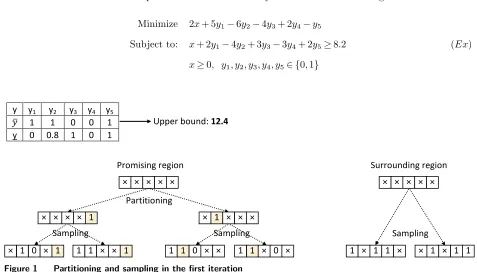
Minimize 2x+ 5y1−6y2−4y3+ 2y4−y5

Subject to: x+ 2y1−4y2+ 3y3−3y4+ 2y5≥8.2 (Ex)

x≥0, y1, y2, y3, y4, y5∈ {0,1}

y y1 y2 y3 y4 y5

𝑦𝑦� 1 1 0 0 1 y 0 0.8 1 0 1

Upper bound: 12.4

Sampling Sampling

Sampling

Partitioning *

× 1 1 1

× × × × ×

Promising region Surrounding region × × × × ×

1 × 1 1 × × 1 × 1 1 × × × × 1 × 1 × × ×

× 1 0 × 1 1 1 × × 1 1 1 0 × × 1 1 × 0 ×

Figure 1 Partitioning and sampling in the first iteration

In the first iteration, suppose the feasible solution candidate y and lower bound solution y shown in

sampling. As we discussed, the binary variablesy2,y4andy5are more likely to be chosen as partitioning and

sampling variables because they have smaller gaps between y and y. In this example, assume there is only

one partitioning variable, and the current most promising region is partitioned into two subregions, η1 =

{×,×,×,×, 1}andη2={×, 1,×,×,×}(×indicates the variable is free). In each of these two subregions,

suppose there are two sampled subproblems, in which two binary variables are chosen as sampling variables;

this leads to four subproblems in the promising region. Let us take the subproblem on the left in Figure 1,

for example, which can be described as follows (other subproblems can be constructed similarly).

Minimize 2x+ 5y1−6∗1−4∗0 + 2y4−1

Subject to: x+ 2y1−4∗1 + 3∗0−3y4+ 2∗1≥8.2

y5=y5= 1, {5} ∈qp (Ex

S1₎

y2=y2= 1, y3=y3= 0, {2,3} ∈qs

x≥0, y1, y4∈ {0,1}

To ensure that all points in the feasible region have a possibility of being evaluated, a random sampling

procedure is performed in the surrounding region. However, less effort is put on this region, as random

sampling is performed directly without first performing partitioning in this region. Let us assume that two

sample problems are identified from the surrounding region (see Figure 1). Three binary variables are first

chosen randomly as sampling variables and their values are also randomly selected. This results in a total of

six subproblems (defined asPS1 _toPS6_{in Figure 1 from left to the right) in the first iteration.}

Let us assume that all of these subproblems and their LP relaxations can be solved to optimality using

methods H and L, respectively; the lower bounds of these subproblems are 11.4, 8, 12.4, 7, 10.4 and 9.4,

respectively. Within each partitioned subregion and in the surrounding region, the subproblem with the

best promise index is identified for further evaluation using its upper bound promise index. Consequently,

subproblemsPS2_,PS4_andPS6_{are identified for further exploration. After solvingP}S2_,PS4 _andPS6 _using

H, their upper bounds are known to be 8, 7 and 9.4, respectively. This indicates that subproblem PS4

has the best upper bound promise index, and this is therefore selected as the most promising subproblem.

Because this subproblem comes from within the promising region, the value of partitioning variable y2 in

the subproblem is fixed, and its index {2} is inserted intoqf. SubproblemPS4 _{has a smaller upper bound}

than the original upper bound. Therefore, the candidate feasible solutiony must be updated to the upper

bound solution ofPS4_{, which is{1, 1, 1, 0, 0}. At the same time, the lower bound solution for the promising}

region must also be updated asy2 has been fixed to 1.

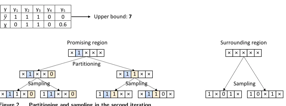
In the second iteration, the procedure is similar to the first one. Suppose we now have the six new

subproblems shown in Figure 2, and that the fourth subproblem from the left has the lowest upper bound,

equal to 3. Therefore, this subproblem is identified as the most promising subproblem. A similar procedure

as before would then be performed until meeting one of the stopping criteria. If at any point a subproblem

in the surrounding region provides the best upper bound promising index, backtracking must be performed,

Author: Article Short Title

Article submitted to ; manuscript no. (Please, provide the mansucript number!) 17

y y1 y2 y3 y4 y5

𝑦𝑦� 1 1 1 0 0

y 0 1 1 0 0.6

Upper bound: 7

Sampling Sampling

Sampling

Partitioning *

× 1 1 1

Promising region Surrounding region

× × × × ×

1 × 0 1 × 1 0 × 1 ×

× 1 × × 0 × 1 1 × ×

× 1 1 × 0 1 1 × × 0 1 1 1 × × 1 0

× 1 × × ×

× 1 ×

Figure 2 Partitioning and sampling in the second iteration

3.3.

The Lower and Upper Bound Guided Nested Partitions Algorithm

To present a step-by-step description of the LugNP method we require the following additional notation:

Θ = The feasible region.

Tlim = The algorithm time limit for the framework. y = The best candidate feasible solution.

y = The best lower bound solution.

σ(k) = The most promising region in thekth_iteration.

PS

kji = Theith subproblem in thejth partition of thekth iteration. qf = The index set containing fixed binary variables.

qpkj = The index set containing partitioning variables in thejthpartition of thekth iteration. qskji = The index set containing sampling variables in theithsubproblem of the jthpartition of the

kth_iteration.

With all the necessary notation in hand, we can now provide a precise description of the LugNP algorithm.

Algorithm LugNP:

Step-I: Initialization.Solve P usingH and Lto obtain an initial feasible solution candidatey and a lower bound solutiony. Setk= 1,qf =∅ and the current most promising region,σ(k) = Θ. Go

to Step-II.

Step-II: Partitioning.LetSσ(k) denote the number of subregions of σ(k). Partition σ(k) intoSσ(k)

subregionsσ1(k), ...,σS_σ(k)(k) by selectingqpkj for each subregionσj(k),j= 1, ..., Sσ(k). Aggregate

the surrounding region Θ\

S_σ(k)

P

j=1

σj(k) into one regionσSσ(k)+1(k). Go to Step-III.

Step-III: Sampling. Let Nj denote the number of subproblems from region σj(k). Use a sampling procedure to selectqskji, i= 1, ..., Nj, in order to construct subproblems from each of the regions σj(k),j= 1,2, ..., Sσ(k)+ 1,; these subproblems are listed as follows:

PS

kj1, PSkj2, ..., PSkjNj, j= 1,2, ..., Sσ(k)+ 1. (29)

Go to Step-IV.

Step-IV: Estimating promising index.Solve all subproblems usingL to obtain lower bounds,

Determine the most promising subproblem within each subregion, where

ˆ_i

kj= arg min i∈{1,...,Nj}

Lo(PSkji), j= 1,2, ..., Sσ(k)+ 1. (31)

Note that ˆikj is the index of the most promising subproblem within subregionσj(k). This results

inSσ(k)+ 1 subproblems, which are solved byH in order to obtain upper bounds.

Hu(PSkj(ˆikj)), j= 1,2, ..., Sσ(k)+ 1. (32)

Determine the most promising subproblem, where

ˆ

jk= arg min

j∈{1,...,S_σ(k)+1}Hu(P S

kj(ˆi_jk)). (33)

Note that ˆjk is the index of the most promising subproblem in thekth iteration, and ˆjk is also the

index of the most promising region to which the most promising subproblem belongs. If two or more

regions are equally promising, ties can be broken arbitrarily. If this index corresponds to a region

that is a subregion ofσ(k), then let this serve as the most promising region in the next iteration.

Note that in this promising region,qp_k(ˆj

k) has been inserted intoqf. Go to Step-V. Otherwise, if the index corresponds to the surrounding region, go to Step-VII.

Step-V: Updating the feasible solution candidate.UpdateytoHy(PSk(ˆjk)(ˆikˆj)) ifHu(P S

k(ˆjk)(ˆikˆj)) is the smallest upper bound so far. Setk=k+ 1. Go to Step-VI.

Step-VI: Stopping criteria check.Ifqf=mor the solution time exceeds the algorithm time limit

Tlim, then the algorithm stops. Lety be the final solution, otherwise, go to Step-II.

Step-VII: Backtracking. Set qf =∅, k = 1. Update the most promising region to Θ, and y to Hy(PSk(ˆjk)(ˆikˆj)) ifHu(P

S

k(ˆjk)(ˆikˆj)) is the smallest upper bound so far. Go to Step-II.

3.4.

Design of the Optimization Framework for the ML-CLSB

This subsection describes the application of the LugNP method to the ML-CLSB problem class. As we noted

before, the LugNP framework offers flexibility in selecting approaches for achieving lower and upper bound

solutions. For obtaining lower bound solutions, standard methods such as LP relaxation, LR, CG, and CP

can be adopted. In the case of ML-CLSB, we directly use the LP relaxation technique (L) to obtain the lower

bound solutions y. For obtaining upper bound solutions, many heuristic algorithms, such as tabu search, relax-and-fix, simulated annealing, and genetic algorithms, can be selected. Because of our focus on lot-sizing

problems, we use a relax-and-fix heuristic (H) technique to achieve upper bound solutionsy.

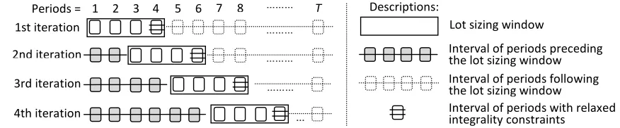
The basic idea of the relax-and-fix algorithm implemented here is to partition all periods in the entire

time horizon into three parts. The first part corresponds to a time window that contains several periods,

the second includes the periods preceding the time window, and the third covers the periods following the

time window. In the early stages of this algorithmic approach, only the lot-sizing problem in the first time

window is solved (here, αis defined as the size of the time window). Within this time window, the binary

variables in the first few periods are required to be binary, and the binary variables in the remaining periods

solver is then used for solving these smaller problems (here, the solving time limit is defined as Trf), with

fewer complicating binary variables, and the resulting solution is used to fix the binary variables in the first

few periods in the time window (here, the size of such periods is defined asβ, withβ≤α-γ). The following

periods (from periodβ+ 1 toβ +α) are then processed in the same manner until all binary variables are

fixed. In the example shown in Figure 3,αequals 4,β equals 2, andγ equals 1.

… … …

Descriptions: Periods = 1

3rd iteration 2nd iteration

1st iteration ………

………

……… 2 3 4 5 6 7 8 ……… T

Lot sizing window

Interval of periods preceding the lot sizing window Interval of periods following the lot sizing window

4th iteration Interval of periods with relaxed _{integrality constraints}

Figure 3 The relax-and-fix algorithm

In the case of the ML-CLSB problem class, subproblems in the LugNP framework are expressed as follows.

Minimize (13)

Subject to: (14),(15),(16),(17),(18)

uitp≥0 ∀i∈[1, I], t∈[1, T], p∈[t, T]. (ZSF LS )

yit=yit, it∈qf∪qp∪qs

yit∈ {0,1}, it∈qm

If we replace problemP with ZSF L, replace problem PS withZSF LS , use the LP relaxation technique as

the lower bound techniqueL, and use the relax-and-fix algorithm as the upper bound techniqueH, then the

LugNP framework expressed above can be implemented to solve the ML-CLSB problem class.

4.

Computational Results

Our computational experiments were conducted on numerous test instances of different sizes, in order to

characterize the performance of LugNP across a wide range of problem instances. Moreover, as noted by

Stadtler (2003), ”once this problem is solvable for some 100 items over a planning interval of 6-12 months

it may well substitute for the current MRP II logic”. Some of the test problems we used for computational

results are based on problems with sizes in this range or even bigger.

4.1.

Description of Test Instances

The first group of test data sets we used was generated by Tempelmeier and Derstroff (1996) and Stadtler

(2003). These data sets include sets A+, B+, C, and D, where A+ contains 120 test instances, B+ contains

312 test instances, C contains 144 test instances, and D contains 79 test instances. Sets A+ and B+ include

periods, and 6 machines. There are no setup times for sets A+ and C, but sets B+ and D include positive

setup times. Moreover, these data sets were constructed using a full factorial design with seven factors as

follows:

1. Operations structure: there are two such settings: general and assembly. Assembly structures have the

limitation that each item has only one ‘child’ item in the BOM, i.e., an item can only be used as a component

of one other item. In a general structure, no such limitation exists.

2. Resource assignment: there are two such settings, acyclic and cyclic. No item is allowed to use the

same machine as one or more of its predecessors for acyclic problems, though such situations are permitted

for cyclic problems. Acyclic problems are generally more difficult to solve than the corresponding cyclic

problems; we only consider acyclic problems.

3. Setup times: there are five such settings denoted by 0, 1, 2, 3, and 4, where 0 indicates that there are

no setup times, and 1, 2, 3, and 4 indicate that setup times are required before producing an item.

4. Coefficient of demand variation: we consider two settings denoted by 1 and 2, where 1 indicates slight

demand variation and 2 indicates sizable variation.

5. Resource utilization: there are five such settings denoted by 1, 2, 3, 4, and 5, where 1 represents high

utilization, 2, 4, and 5 represent medium utilization, and 3 corresponds to low utilization.

6. TBO: TBO denotes the time between orders, and we consider three such settings denoted as 2, 3 and

4, where 2 indicates a high TBO, 3 indicates a medium TBO, and 4 corresponds to a low TBO.

7. Amplitude of seasonal pattern: we consider three settings denoted by 0, 1, and 2, where 0 indicates no

seasonality for item demands, 1 indicates slight seasonality, and 2 indicates strong seasonality.

For more details about these instances, see Tempelmeier and Derstroff (1996) and Stadtler (2003).

Origi-nally, these data sets had no allowance for backlogging; we thus slightly alter the problem instances in order

to permit backlogging. We use a ratio of backlogging costs to inventory costs such that bci = 10*hci for

i∈endp. The resulting data sets are referred to asA+,B+,C, andD, after this modification.

We generated an additional group of data sets based on the above sets, in which, for each test instance,

the demand for all items increases by twenty percent for the first half of the time horizon, while the resource

capacities increase by ten percent over the time horizon. This new group of data sets was generated so that

backlogging plays a more significant role. The resulting data sets are referred to asA+,B+,C, andD.

The third group of test data sets we used was generated by Simpson and Erenguc (2005) and Akartunalı

and Miller (2009). These data sets include sets SET1, SET2, SET3, and SET4, each set having 30 instances

with low, medium and high variability of demand. This group of data sets was originally generated without

backlogging; Akartunalı and Miller (2009) later modified the data sets by adding backlogging costs to them.

The backlogging costs are set to twice the inventory holding costs for the first two sets, and 10 times the

inventory holding costs for the last two sets. Except for the problems in SET2, which have a horizon of

24 periods, all instances have 16 periods. All instances have 78 items and have an assembly structure, and

backlogging is allowed in the last period. For more details about the instances, see Simpson and Erenguc

4.2.

Settings for Computational Tests

We compare the LugNP procedure with the heuristic method proposed by Akartunalı and Miller (2009)

(denoted by Aheur) and the commercial MIP solver CPLEX 11.2 (B&C) in order to establish its efficiency

relative to state-of-the-art methods. The very efficient algorithm proposed by Akartunalı and Miller (2009)

is able to obtain excellent results for lot-sizing problems, and is the only algorithm in the extant literature

that has been implemented to solve ML-CLSB. The commercial MIP solver, CPLEX 11.2, is one of the

most powerful solvers with the branch-and-cut algorithm embedded. This solver is very efficient at solving

lot-sizing problems. In order to ensure fair comparisons, all three approaches were implemented on the same

SFL model, and the same computing capacity (Intel Pentium 4, 3.16 GHz processor) was used. Each of these

approaches was programmed using GAMS, a high-level algebraic modeling language, in which CPLEX 11.2

is called as the solver.

A total computing time of 100 seconds was allocated for instances in sets A+,B+,A+,B+, and SET1,

and 300 seconds for instances in setsC,D,C,D, SET3, and SET4 (because of the complexity). A computing

time of 150 seconds was allocated for instances in set SET2, due to the particularly bad results achieved

by Aheur when the time was set to 100 seconds. The total time assigned to the three approaches is the

same; so this comparison is reasonable and valid. There are many possible parameter settings, even when

the total solution time is limited for each of the above approaches. One possible setting that might maximize

the performance of the corresponding approach is based on empirical data. First, for LugNP, values of α,

β, and γ are set to d5 +Tlim/300e, 2, and 2, respectively, for obtaining the initial upper bound solutions,

while the value ofαis altered to the total length of the entire horizon when solving the subproblems,ZN P SF L. The number of partitioning variables at any iteration is set to 2, and the number of sampling variables at

any iteration is set to max I×T₂ ,|qm| ∗0.6in the dth iteration. Trf is set to 1 +Tlim/100 seconds for data sets A+,B+, A+,B+, and set to 5 + Tlim/100 seconds otherwise. The number of partitioned subregions

within the promising region at any iteration is set to 10, the number of sample problems in each partitioned

subregion at any iteration is set to 3, and the number of sample problems in the surrounding region at any

iteration is set to 1. Second, in Aheur, the strategy recommended by Akartunalı and Miller (2009) is applied

to set parameter values; details are omitted here. Finally, for the CPLEX solver, the “flow cover” and “Mixed

Integer Rounding (MIR)” cuts are activated to improve solution quality.

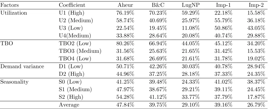
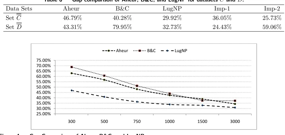
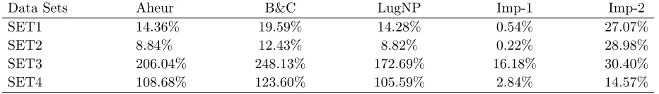
The computational results in terms of duality gaps are given in the Tables 1-3. The duality gap is calculated

as the difference between upper and lower bound values, divided by the lower bound value. For a fair

comparison, the lower bound yielded by the LP relaxations of SFL was used for calculating the duality

gaps for all three approaches. As the same lower bound is used for all three approaches, the comparison

of duality gaps also can be considered as a comparison of cost savings. In these tables, Imp-1 indicates

the improvement brought about by LugNP, compared with Aheur, while Imp-2 denotes the improvement

compared with B&C. Imp-1 is calculated as (Aheur’s duality gap−LugNP’s duality gap)/(Aheur’s duality

gap); Imp-2 is calculated in the same manner. The first two tables provide details of the computational

results for different problem characteristics, whereas Table 3 provides a summary. As these results indicate,

Table 1 Gap comparison of Aheur, B&C, and LugNP for the full factorial experiment of dataset A+.

Factors Coefficient Aheur B&C LugNP Imp-1 Imp-2

Utilization U1 (High) 54.91% 50.09% 41.71% 24.05% 16.74%

U2 (Medium) 27.44% 32.61% 21.79% 20.57% 33.16%

U3 (Low) 12.27% 14.63% 10.92% 11.04% 25.37%

U4(Medium) 25.04% 29.64% 22.56% 9.91% 23.91%

U5(Medium) 31.38% 34.24% 26.83% 14.48% 21.63%

TBO TBO3 (Medium) 32.89% 33.79% 27.01% 17.86% 20.06%

TBO4 (Low) 27.53% 30.69% 22.51% 18.23% 26.66%

Demand variance D1 (Low) 30.02% 32.62% 24.63% 17.96% 24.48%

D2 (High) 30.39% 31.86% 24.89% 18.10% 21.88%

Seasonality S0 (Low) 25.91% 28.64% 21.48% 17.10% 25.01%

S1 (Medium) 30.64% 33.40% 24.25% 20.86% 27.40%

S2 (High) 34.08% 34.68% 28.56% 16.19% 17.66%

Average 30.21% 32.24% 24.76% 18.03% 23.20%

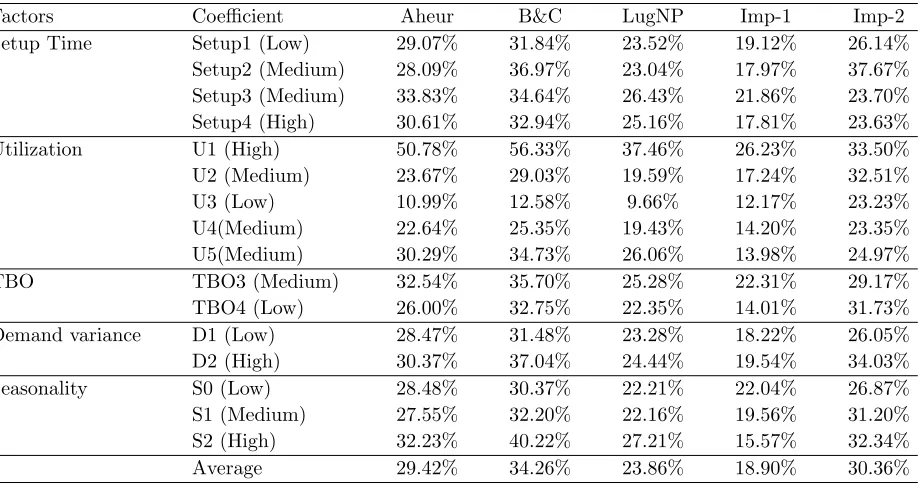
Table 2 Gap comparison of Aheur, B&C, and LugNP for the full factorial experiment of datasetB+.

Factors Coefficient Aheur B&C LugNP Imp-1 Imp-2

Setup Time Setup1 (Low) 29.07% 31.84% 23.52% 19.12% 26.14%

Setup2 (Medium) 28.09% 36.97% 23.04% 17.97% 37.67%

Setup3 (Medium) 33.83% 34.64% 26.43% 21.86% 23.70%

Setup4 (High) 30.61% 32.94% 25.16% 17.81% 23.63%

Utilization U1 (High) 50.78% 56.33% 37.46% 26.23% 33.50%

U2 (Medium) 23.67% 29.03% 19.59% 17.24% 32.51%

U3 (Low) 10.99% 12.58% 9.66% 12.17% 23.23%

U4(Medium) 22.64% 25.35% 19.43% 14.20% 23.35%

U5(Medium) 30.29% 34.73% 26.06% 13.98% 24.97%

TBO TBO3 (Medium) 32.54% 35.70% 25.28% 22.31% 29.17%

TBO4 (Low) 26.00% 32.75% 22.35% 14.01% 31.73%

Demand variance D1 (Low) 28.47% 31.48% 23.28% 18.22% 26.05%

D2 (High) 30.37% 37.04% 24.44% 19.54% 34.03%

Seasonality S0 (Low) 28.48% 30.37% 22.21% 22.04% 26.87%

S1 (Medium) 27.55% 32.20% 22.16% 19.56% 31.20%

S2 (High) 32.23% 40.22% 27.21% 15.57% 32.34%

Average 29.42% 34.26% 23.86% 18.90% 30.36%

Table 3 Gap comparison of Aheur, B&C, and LugNP for datasetsA+andB+.

Data Sets Aheur B&C LugNP Imp-1 Imp-2

SetA+ 28.98% 30.82% 24.92% 13.99% 19.12%

SetB+ 34.30% 34.69% 28.57% 16.69% 17.63%

4.3.

Computational Results for Test Instances of Medium Size

According to the results shown in Tables 1 and 2, the level of capacity usage has a significant influence

on the duality gap for all three approaches. For example, the duality gaps for highly capacitated problems

are about four times the gaps for less capacitated problems. In addition, TBO and seasonality also have a