Adaptive Backstepping Control for Optimal Descent
with Embedded Autonomy
Maodeng Li∗, Wuxing Jing
Department of Aerospace Engineering, Harbin Institute of Technology, Harbin,
Heilongjiang, 150001, China
Malcolm Macdonald, Colin R McInnes
Advance Space Concepts Laboratory,University of Strathclyde, Glasgow, Scotland, G1 1XJ, E.U.
Abstract
Using Lyapunov stability theory, an adaptive backstepping controller is pre-sented in this paper for optimal descent tracking. Unlike the traditional ap-proach, the proposed control law can cope with input saturation and failure which enables the embedded autonomy of lander system. In addition, this control law can also restrain the unknown bounded terms (i.e., disturbance). To show the controller’s performance in the presence of input saturation, input failure and bounded external disturbance, simulation was carried out under a lunar landing scenario
Keywords:
Adaptive backstepping control, Input failure, Input saturation, Optimal descent
∗Corresponding author
1. Introduction
Over the past four decades, many studies on the guidance of planetary descent have been extensively reported in the literature [1–6]. Among those approaches, the tangent optimal guidance law [4, 5, 7–9] has been investi-gated widely. The advantage of this steering law is that it is derived from optimal control theory, therefore it can achieve fuel optimal (suboptimal). In general, a closed form solution for this guidance law cannot be found for the full model [5]. An effective method to approach the optimal solution is restricting the acceleration profile in a polynomial function in each axis [4, 5, 7], the analytic equations of velocity and position can be integrated from the acceleration profile. Therefore, the guidance acceleration can be solved from boundary conditions. Another method is developing a closed form solution for the simplified model of the full model initially, and then designing a control law to track the developed closed form solution [8, 9].
However, much of above-mentioned works assume the actuator to work perfectly. In fact, the actuator is often subjected to saturation, while actuator failure may also occur. Therefore, the derivation of a controller for planetary optimal descent in the presence of input saturation and failure is an important issue.
systems.
The rest of this paper is organized as follows: In Section 2, the dynamics of the descent are presented. In addition, the optimal linear tangent law and a closed form solution based on a simplified model are also introduced in Section 2. Section 3 develops an adaptive backstepping controller for a class of nonlinear system with multiple input in the presence of input saturation and failure. Thereafter, the optimal descent control law is illustrated in Section 4. Section 5 shows the simulation results and discussion. Finally, conclusions are provided in Section 6.
2. Optimal Descent
The dynamics of descent can be described as follows [4],
˙
r = −w (1a)
˙
ϕ = 1
ru (1b)
˙
λ = 1
rcosϕv (1c)
˙
u = −v
2
r tanϕ+
uw
r +
Tx
m (1d)
˙
v = uv
r tanϕ+
vw
r +
Ty
m (1e)
˙
w = −u
2+v2
r +
µ
r2 +
Tz
m (1f)
˙
m = −T /(IspgE) (1g)
velocity in vehicle carried local vertical frame FH [9],
Tx
Ty
Tz
=
−T cosαBcosψB
−T cosαBsinψB
−T sinαB
(2)
is the thrust vector expressed in FH,T is the thrust vector magnitude, ψB is lander’s yaw angle, αB is lander’s pitch angle, m is the lander’s mass, Eq. 1g is the mass flow equation with Isp the lander’s specific impulse (impulse per unit weight-on-Earth of propellant) and gE the gravitational acceleration on the Earth’s surface.
For a landing mission in which boundary height and velocity are specified, it is well known that the tangents of the optimal attitude angles are linear functions of time which can be described as follows [4, 5],
tanψB = a1 (3a)
tanαB = a2t+a3 (3b)
where, ai (i= 1,2,3) are unknown constants to be solved.
Neglecting small terms−v2/rtanϕ,uw/r,uv/rtanϕ, anduw/rin Eq. (1)
trajectory can be solved as a closed form [9],
ud(t) =
n
∑
i=0
uiti (4a)
vd(t) = a ud(t) (4b)
wd(t) =
n−1
∑
i=0
witi (4c)
hd(t) =
n
∑
i=0
hiti (4d)
where ui, wi, and hi are functions of unknown constants ai (i= 1,2,3), and subscript d indicates desired values. Therefore, the unknown constants ai (i = 1,2,3) can be solved from boundary conditions of height and velocity and the closed form guidance trajectory can be solved as well.
3. Adaptive Backstepping Control
Consider a class of dynamic systems with the form of
˙
x1 = f1(x1)x2 (5a)
˙
x2 = f2(x1, x2) +d+B0u (5b)
where x1 ∈ Rn1 and x2 ∈ Rn2 are the state variables, f1 ∈ Rn1×n2 is a
matrix of continuously differentiable nonlinear functions,f2 ∈Rn2 is a known
smooth nonlinear function,dis a unknown bounded time-varying disturbance or an uncertain term, u ∈ Rm is the actual control input and B0 is the
coefficient matrix of control input.
In practice, if the control input is subjected to saturation and control failure may occur, the actual input u can be written as
u=fa(sat(uc)) (6)
where uc is the command input, sat(·) is the saturation function and fa describes the failure mode.
A control law is now required with the property that all states of the system in Eq. (5) are bounded and stable at x1, x2 = 0, i.e., x1, x2 → 0 as
t → ∞.
It will be shown that the control law for command input
uc =−B0†(F2(x2−p) +f1⊤x1+f2−p˙+
d20ez2
∥z2∥d0e+ ¯f3∥z2∥2
) (7)
possesses these properties, where B0† is the Moore-Penrose pseudoinverse of
B0 ( The definition of Moore-Penrose pseudoinverse can be found in Ref. [14]
), F2 is a positive definite matrix, 0<f¯3 <f¯2 and ¯f2 >1/2 is the minimum
matrix, d0e is an estimate of ∥d∥which is obtained from
˙
d0e=q∥z2∥ (8)
where q >0.
Next the derivation of the control law will be given. The following trans-formation is introduced to compensate the effect of input saturation and failure:
z1 = x1−λ1 (9a)
z2 = x2−λ2−p (9b)
where λ1 and λ2 are virtual states,p is the virtual control, which is designed
as,
p=−K1f1⊤x1 (10)
and K1 is chosen that F1 :=f1K1f1⊤ is a positive definite matrix.
The virtual statesλ1 and λ2 are chosen to satisfy the following equations:
˙
λ1 = −F1λ1+f1λ2 (11a)
˙
λ2 = −F2λ2−f1⊤λ1+B0∆u (11b)
where ∆u=u−uc and F2 is a positive matrix. The initial values of λ1 and
λ2 are chosen as λ1(0) = 0, λ2(0) = 0.
The candidate of Lyapunov function is chosen as,
V2 =
1 2z
⊤
1 z1+
1 2z
⊤
2 z2+
1 2q
ˆ
where ˆd0 =d0e− ∥d∥.
Substituting Eq. (10), Eq. (8), Eq. (11) and control law Eq. (7) into the derivation of V2 along with z system, the following inequality is derived,
˙
V2 ≤ −z1⊤F1z1−z2⊤F2z2+ ¯f3∥z2∥2
≤ −f¯1∥z1∥2−
( ¯f2−f¯3)∥z2∥2 (13)
where ¯f1 > 0 is the minimum eigenvalue of F1. To use LaSalle-Yoshizawa
Theorem [13], the designed parameters ¯f2 and ¯f3 are chosen as ¯f2 >f¯3 >0.
Using LaSalle-Yoshizawa Theorem, it is shown that
lim
t→∞z1 = tlim→∞(x1−λ1) = 0 (14a) lim
t→∞z2 = tlim→∞(x2−p−λ2) = 0 (14b) To see the convergence ofx1, x2, the candidate of Lyapunov function ofλi(i= 1,2) system is chosen as,
Vλ =
1 2λ
⊤
1λ1+
1 2λ
⊤
2λ2 (15)
Then, the derivative of Vλ along Eq. (11) can be given by
˙
Vλ = −λ⊤1F1λ1−λ2⊤F2λ2+λ⊤2B0∆u (16)
If no input saturation and failure occur, ∆u= 0. Using LaSalle-Yoshizawa Theorem, it is shown that limt→∞λ1 = 0 and limt→∞λ2 = 0. Then, from
Eq. (14a) it is seen that limt→∞x1 = 0. Thereafter, from Eq. (10) it is seen
that limt→∞p = 0. Then from Eq. (14b), it is shown that limt→∞x2 = 0
If input saturation and failure occur, ∆u ̸= 0. To show boundedness of
λ1 and λ2, Eq. (16) can be written as,
˙
Vλ = −λ⊤1F1λ1−λ2⊤F2λ2+λ⊤2B0∆u (17a)
≤ −f¯
1λ⊤1λ1−( ¯f2−0.5)λ⊤2λ2+
1
2(B0∆u)
⊤B
0∆u (17b)
To use Lasalle-Yoshizawa Theorem, the design parameter ¯f2 is chosen as
¯
f2 >0.5 such that the second term of the above equation is negative.
Integrating Eq. (17), the following equation is given
∥λ1∥2 ≤
1
√
2 ¯f1
∥B0∆u∥ (18a)
∥λ2∥2 ≤
1
√
2 ¯f2−1
∥B0∆u∥ (18b)
From Eq. (13), it is shown that
∥z1∥22 =
∫ ∞
0
z1⊤z1 dt≤
1 ¯
f1
V2(0) (19a)
∥z2∥22 =
∫ ∞
0
z2⊤z2 dt≤
1 ¯
f2
V2(0) (19b)
where
V2(0) =
1 2z1(0)
⊤z
1(0) +
1 2z2(0)
⊤z
2(0) (20)
with z1(0) =x1(0), and z2(0) =x2(0)−A1f1⊤x1(0).
From Eq. (18) and Eq. (19), the bounds of the transient tracking errors can be written as
∥x1∥2 ≤
1
√
2 ¯f1
(√2V2(0) +∥B0∆u∥) (21a)
∥x2∥2 ≤
1
√
¯
f2
√
V2(0) +
1
√
2¯c2
x 1
x 2
∆u
λ system λ1
λ 2
Eq.(11)
z system
Eq.(9) Eq.(8) d0e
Eq.(10),Eq.(5a)
p,p˙
z1, z2
z2
Eq.(7) uc Actuator
u
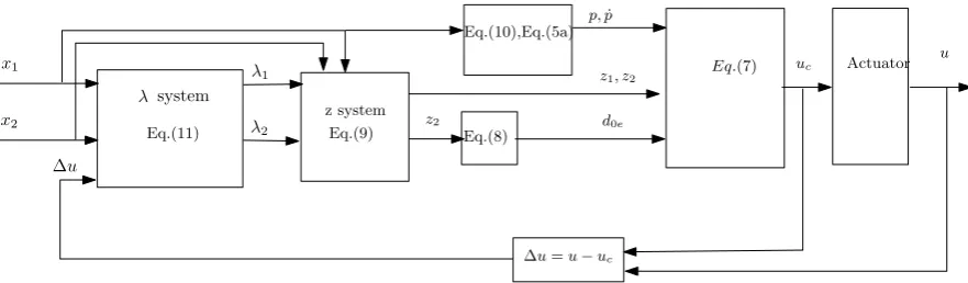
[image:10.595.117.558.124.253.2]∆u=u−uc
Figure 1: Flow chart of the implementation of the controller
Furthermore, the performance of control can be improved by increasing the parameters ¯f1 and ¯f2. For sufficiently large ¯f1 and ¯f2, then x1, x2 → 0 as
t → ∞.
The flow chart of the implementation of the controller is shown in Fig. 1. Firstly, the values λi (i=1,2) are integrated from Eq.(11). The values of p and ˙p are calculated from Eq. (10) and Eq. (5). Thereafter, the values of
4. Optimal Descent Control Law
Now that the general control law has been presented, an adaptive back-stepping control law is developed. The design of navigation system is not considered in this paper. It is assumed that the values of states can be ob-tained from the inertial navigation system and the control law is to track the predefined profile in Eq. (4).
For the orbit tracking, a height error and velocity error are defined as
eh(t) = h(t)−hd(t) and ev(t) = V(t)−Vd(t), respectively. Then the error equation of height and velocity can be written as,
˙
eh(t) = ahev(t) (22a) ˙
ev = do−1/m uo (22b)
where ah = [0,0,−1],do is nonlinear terms, and
uo =
T cosαBcosψB−TdcosαBdcosψBd
T cosαBsinψB−TdcosαBdsinψBd
T sinαB−TdsinαBd
(23)
The saturation function can be written as
sat(uco) =
(uco+unorm)Tmax/T −unorm |uco+unorm| ≥Tmax
uco |uco+unorm|< Tmax
(24)
where uco is the command input for orbit tracking, Tmax is the saturation level of thrust andunorm is the nominal control input which can be described as follows,
unorm =
TdcosαBdcosψBd
TdcosαBdsinψBd
TdsinαBd
Furthermore, if 30% of thrust is assumed to fail at the midpoint of descent, the actual thrust level equals command thrust level when t ≤tf/2 and the actual thrust level is 70% of the command thrust when tf/2 < t ≤ tf. Using the special continues function tan−1 to approach this characteristic, the failure mode can be written as [3],
fa =
1 +Ta 2 (1−
2
π
1−Ta 1 +Ta
tan−1(2t−tf))(uco+unorm)−unorm (26)
where Ta = 0.7.
It is shown that Eq. (22) is of the form of Eq. (5) with x1 =eh, x2 =ev,
f1 = ah, f2 = 0, d = do and B0 = −1/m. Then the controller Eq. (7) and
update law Eq. (8) can be implemented directly.
For the numerical simplicity of the on-board real time computations, quaternion is used for the attitude tracking. The quaternion from FH to body frame FB [9] is defined as Q = [q0, q⊤]⊤, where q0 is a scalar part
of the quaternion, and q = [q1, q2, q3]⊤ is the vector part. The reference
frame of attitude corresponding to the commanded motion is denoted by
FBd and its attitude with respect to FH is specified by the unit quaternion
Qd = [q0d, qd⊤]⊤ which is transformed from the Euler angles derived from orbit tracking system using Eq. (5.13) and Eq. (5.38) in Ref. [15]. The error of quaternion eQ := [eq0, e⊤q]⊤ and angular velocity of lander are then defined as [10] eQ = ¯Qd ⊗Q and eω = ω−L(eQ)ωd, respectively, where
¯
Qd = [q0d,−qd⊤]⊤ is the inverse of Qd and L(eQ) is the rotation matrix from
dynamics and kinematics can be expressed as,
˙
eq =
1
2[eq0I3 +S(eq)]eω (27a) ˙
eω = −J−1(Crω+nr)−ndo+J−1M +J−1dM (27b)
where, J is the inertia matrix of lander, S(•) is cross-product operator [10],
M is the control torque,
Cr(ω) = J S(LBHωHHP)−S(J(ω+LBHωHHP)) +S(LBHωHHP)J
nr(ω) = S(LBHωHPH )J(LBHωHHP) +J LBH
dωH
HP
dt + ˙J(ω+LBHω
H HP)
ndo = S(eω)L(eQ)ωd+L(eQ) ˙ωd
withLBHthe rotation matrix fromFH toFBandωHPH = [ ˙λcosϕ,−ϕ,˙ −λ˙ sinϕ]⊤ the angular velocity of FH with respect to planetary fixed frame FP [9] expressed in FH, dM is the bounded external disturbance torque. If the
J = J0 + ∆J, where J0 and ∆J are the certain term and uncertain term of
J, respectively, then the term in Eq. (27) can be also treated as unknown bounded disturbance.
If each axis of torque is subjected to saturation, the saturation function can be written as
sat(Mc)(i) =
sign(Mc(i))Mmax |Mc(i)| ≥Mmax
Mc(i) |Mc(i)|< Mmax
(28)
where i= x, y, z, Mc is the command control torque and Mmax is the satu-ration value of torque.
It can be seen that Eq. (27) is of the form of Eq. (5) withx1 =eq,x2 =eω,
f1 = 1/2[eq0I +S(eq)], f2 = −J−1(Crω+nr)−ndo, B0 = J−1, u =M, and
d=J−1d
5. Results and Discussion
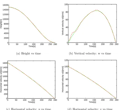
In this section, a numerical simulation of a sample lunar soft landing scenario is given to demonstrate the proposed control law. Nominal initial conditions of optimal descent areh0 = 15 km andV0 = [1609.08,100,0] m/s.
The initial height error is set to be 100 m and initial velocity error is set to [2,3,5]⊤ m/s. Since the terminal guidance will be used following the optimal guidance, the terminal height of optimal descent is specified as hf = 100 m to allow for a further study of terminal descent and the terminal velocity is specified asVf = [0,0,0] m/s. The assumed initial mass is 5156 kg, the nom-inal level of orbit thrust is 24 kN. In addition, the failure mode in Eq. (26) is adopted in numerical simulation. To compensate the thrust failures, a certain of redundancy is necessary [17]. Therefore, the saturation level of orbit thrust is chosen as 34 kN. The specific impulse of orbit thrust is Isp = 315 s. The moment of inertia matrix isJ =diag[2.865,1.826,1.826]×103 kg·m2. For the
attitude tracking, the initial quaternion is chosen asQ0 = [
√
0.8,√0.2,0,0]⊤ and the initial angular velocity is chosen as ω0 = [0,0,0]⊤. The saturation
level of control torque and the external disturbance torque are chosen as 200 Nm and 20[cost,sint,cos 2t]⊤ Nm, respectively. The control parameters for orbit tracking are chosen as K1 = diag[0.1,0.1,0.1], F2 = diag[1,1,20],
¯
f3 = 0.25, d0e(0) = 0, and q = 0.01. The control parameters for atti-tude tracking are chosen as K1 = diag[1,1,1], F2 = diag[5,5,5], ¯f3 = 0.1,
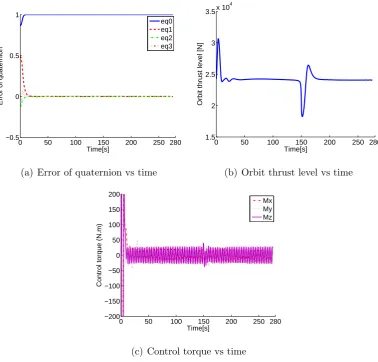
solid line represents the scalar part of the error quaternion and the dashed, dashdot, dotted line represents the vector part of the error quaternion. It can be seen that the initial state error is removed by throttling down the orbit thrusters and adjusting the values of control torques. Figure 3(b) shows the time history of the orbit thrust level. As seen from Fig. 3(b), the control law can adjust the orbit thrust level automatically after the orbit thrust failure occurs. The time history of the control torque is shown in Fig. 3(c), where the dashdot, dotted, and solid line represent the control torque in the direc-tion of x-axis, y-axis, and z-axis, respectively. As seen from Fig. 3(c), since the control torques are mainly used to reject bounded external disturbance after transient response, the estimation of ∥d∥ is about 20 N.m which is the exact value of ∥d∥. Therefore, the control torques can cope with bounded external time-varying disturbance. It is also shown that the the orbit thrust saturation doesn’t occur since enough redundancy is supplied to compensate the thruster failure where the control torque saturation occurs initially. How-ever, the performance of tracking is assured since the control law can cope with thruster failure and saturation. Thus, the proposed controller enables embedded autonomy as it provides a robust approach to deal with failures without requiring the traditional Fault Detection, Isolation, and Recovery (FDIR) system.
6. Conclusions
0 50 100 150 200 250 280 0 2000 4000 6000 8000 10000 12000 14000 16000 Height[m] Time[s]
(a) Height vs time
0 50 100 150 200 250 280
0 20 40 60 80 100 Time[s]
Vertical velocity v(t)[m/s]
(b) Vertical velocity: w vs time
0 50 100 150 200 250 280
0 200 400 600 800 1000 1200 1400 1600 Time[s]
Horizontal velocity u(t)[m/s]
(c) Horizontal velocity: u vs time
0 50 100 150 200 250 280
0 20 40 60 80 100 120 Time[s]
Horizontal velocity v(t)[m/s]
[image:16.595.112.500.117.474.2](d) Horizontal velocity: v vs time
Figure 2: Numerical results of height trajectory and velocity trajectory (--, required profile;
-., Adaptive backstepping Control)
Re-0 50 100 150 200 250 280 −0.5
0 0.5 1
Time[s]
Error of quaternion
eq0 eq1 eq2 eq3
(a) Error of quaternion vs time
0 50 100 150 200 250 280
1.5 2 2.5 3 3.5x 10
4
Time[s]
Orbit thrust level [N]
(b) Orbit thrust level vs time
0 50 100 150 200 250 280
−200 −150 −100 −50 0 50 100 150 200
Time[s]
Control torque (N.m)
Mx My Mz
[image:17.595.116.495.126.488.2](c) Control torque vs time
Figure 3: Numerical results of error quaternion and control input
hardware-in-the-loop simulation, i.e. to run the algorithms on an actual flight processor, and perhaps in a high-fidelity simulations environment capable of performing monte-carlo campaigns.
Acknowledgments
This work has been supported by the Chinese Nature Science Foundation under grant No. 60535010.
References
[1] R. Cheng, Lunar terminal guidance, in: Lunar Missions and Explo-ration, Wiley, New York, 1964.
[2] S. Citron, S. Dunin, H. Meissinger, A terminal guidance technique for lunar landing, AIAA Journal 2 (3) (1964) 503–509.
[3] C. McInnes, Direct adaptive control for gravity-turn descent, Journal of guidance, control, and dynamics 22 (2) (1999) 373–375.
[4] S. Ueno, Y. Yamaguchi, 3-dimensional near-minimum fuel guidance law of a lunar landing module, in: Proceeding of AIAA Guidance, Naviga-tion, and Control Conference, Portland, OR, 1999, pp. 248–257.
[5] R. R. Sostaric, J. R. Rea, Powered descent guidance methods for the moon and mars, in: Proceeding of AIAA Guidance, Navigation, and Control Conference, San Francisco, California, 2005.
[7] D. Wang, X. Huang, Y. Guan, GNC system scheme for lunar soft landing spacecraft, Advances in Space Research 42 (2008) 379–385.
[8] H. Afshari, J. Roshanian, A. Novinzadeh, A perturbation approach in determination of closed-loop optimal-fuzzy control policy for planetary landing mission, Proceedings of the Institution of Mechanical Engineers, Part G: Journal of Aerospace Engineering 223 (3) (2009) 233–243.
[9] M. D. Li, M. Macdonald, C. R. McInnes, W. X. Jing, Analytical lunar landing trajectories for embedded autonomy, Proceedings of the Insti-tution of Mechanical Engineers, Part G: Journal of Aerospace Engineer-ing(In press).
[10] R. Kristiansen, P. Nicklasson, J. Gravdahl, Satellite Attitude Control by Quaternion-Based Backstepping, IEEE Transactions on Control Sys-tems Technology 17 (1) (2009) 227–232.
[11] C. Y. Li, W. Jing, C. Gao, Adaptive backstepping-based flight control system using integral filters, Aerospace Science and Technology 13 (2-3) (2009) 105–113.
[12] I. Ali, G. Radice, J. Kim, Backstepping Control Design with Actuator Torque Bound for Spacecraft Attitude Maneuver, Journal of guidance, control, and dynamics 33 (1) (2010) 254–259.
[13] J. Zhou, C. Wen, Adaptive backstepping control of uncertain systems, Springer, 2008.
[15] B. Wie, Space vehicle dynamics and control, Reston, VA: American Institute of Aeronautics and Astronautics, Inc, 1998.
[16] R. Kristiansen, E. Grotli, P. Nicklasson, J. Gravdahl, A model of rel-ative translation and rotation in leader-follower spacecraft formations, Modeling, Identification and Control 28 (1) (2007) 3–13.