Transient analysis of interline dynamic voltage restorer using dynamic phasor representation

1

Transient analysis of interline dynamic voltage

restorer using dynamic phasor representation

Abstract- Computer planning and simulation of power systems require system components to be represented mathematically. A method for building a dynamic phasor model of an Interline Dynamic Voltage Restorer (IDVR) is presented, and the resulting model is tested in a simple radial distribution system. Mathematical analysis is carried out for each individual component of the IDVR as modular models, which are then aggregated to generate the final model. The proposed technique has the advantage of simplifying the modelling of any flexible AC transmission system (FACTS) device in dynamic phasor mode when compared to other modelling techniques reported in the literature. The IDVR, including the series injection transformer, is analysed in both ABC and DQ dynamic phasor modes, and IDVR power management is also presented. The ensure compatibility with transient stability programs, the analysis is performed for the fundamental frequency only, with other frequency components being truncated and without considering harmonics. Results produced by the IDVR dynamic phasor model are validated by comparison with results gained from a detailed MATLAB/Simulink IDVR model.

Keywords: Interline dynamic voltage restorer, generalised average modelling, dynamic phasor model, detailed model, Park’s transformation.

1. Introduction

Different modelling techniques, such as detailed modelling, phasor modelling, average modelling and dynamic phasor modelling, have been introduced in the literature to model power system components. Detailed models reflect most of the power component characteristics, such as the electromagnetic and electromechanical behaviour. However they increase the computational time required to represent the response of the component, thereby imposing a practical limitation on the number of components that can be simulated simultaneously and the size of studied systems [1]. Alternatively, the dynamic phasor representation, which is extracted from the system time domain equations (differential equations) by application of the generalised average procedure [2], offers numerous benefits

compared to traditional modelling approaches. It is more appropriate for fast numerical simulation where the dynamic phasor variable tends to change slowly even under quick system variations, and to a constant value during steady-state operation. This feature shows effectively the relationships between the different elements of the model. In addition, this approach lies between the traditional quasi-steady modelling and detailed time domain modelling techniques [3, 4].

Since the first implementation of dynamic phasor modelling in 1991, it has been successfully applied to different kinds of power components and applications, including flexible AC transmission system (FACTS) modelling and applications (STATCOM, UPFC, TCSC, SVC…)[5, 6], High voltage DC (HVDC) applications [4] and ac machines [7]. Despite the considerable amount of research on this subject, it does not address dynamic phasor modelling of the interline dynamic voltage restorer (IDVR). Additionally, analysis focuses on integrated systems, where it becomes impossible in most cases to generalise the model for other FACTS device modelling applications. Modular models that can represent a variety of power system components and topologies using the dynamic phasor approach will therefore simplify modelling and analysis. A library of dynamic phasor models covering various power system components and their topologies, using the minimum number of building blocks, can therefore be developed.

The IDVR is analysed and a model constructed using separate building blocks (i.e. a modular representation) to provide a better understanding of each IDVR component, and to facilitate the construction of any other FACTS topologies without the need to re-analyse the general construction of that device.

2

2. General construction of an IDVR

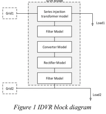
The general construction of an IDVR is presented in Figure 1. As shown, the interline topology allows the load voltage to be compensated through a neighbouring feeder or feeders using back-to-back converters with a common DC link. Even though the IDVR control system is more complex than that of an ordinary DVR, it supports the feeder under fault without excessive loading of that feeder. Moreover, this topology makes the IDVR effective under different balanced and unbalanced voltage sag/swell conditions and enables load voltage compensation for unlimited time [8].

Series injection transformer model

Converter Model Filter Model IDVR Model

Load1

Rectifier Model

Filter Model

Load2 Grid2

Grid1

Figure 1 IDVR block diagram

3. Dynamic phasor representation

Dynamic phasor modelling was developed based on generalised average modelling using the time varying Fourier coefficient in complex form [9]. Any complex periodic waveform 𝑥(𝜏) defined during interval 𝜏 ∈ (𝑡 − 𝑇, 𝑡) can be described using a Fourier series as

𝑥(𝜏) = ∑∞ 𝑋_𝑘(𝑡)𝑒𝑗𝑘𝜔𝑠𝜏

𝑘=−∞ (1)

where 𝜔_𝑠 is the angular frequency, 𝑘 is the harmonic order and 𝑋_𝑘(𝑡) represents the dynamic phasor parameter ‘complex Fourier coefficient’ which can be determined from (2).

𝑋𝑘(𝑡) =_𝑇1∫_𝑡−𝑇𝑡 𝑋(𝜏)𝑒−𝑗𝑘𝜔𝑠𝜏𝑑𝜏 = 𝑥𝑘 (2) Solving systems using dynamic phasor models requires two properties which are:

 The dynamic phasor model of a derivative of the time variable is

〈𝑑𝑥

𝑑𝑡〉𝑘= 𝑑〈𝑥〉

𝑑𝑡 + 𝑗𝑘𝜔𝑠〈𝑥〉𝑘 (3)

 The product of two time domain variables is

〈𝑥𝑦〉𝑘 = ∑∞𝑖=−∞〈𝑥〉𝑘−𝑖〈𝑦〉𝑖 (4)

In general, transforming a system from the time domain to a dynamic phasor representation is achieved as follows:

 Derive the time domain differential equation of the systems or device.

 Apply equations (1) to (4) to transform the system to the dynamic phasor form.

 Truncate unnecessary frequencies to represent the systems.

4. Mathematical analysis of an IDVR

The mathematical models of the three main components of an IDVR, namely the AC/DC and DC/AC converters, the harmonic filter and the series injection transformer, are derived based upon ABC and DQ coordinates respectively .

4.1 ABC DYNAMIC PHASOR MODELLING

I. AC/DC CONVERTER

The general construction of a back-to-back converter is presented in Figure 2. Both converters 1 and 2 (rectifier and inverter) are analysed in the same way, so for simplicity the subscripts (1 and 2) are omitted during the analysis.

Vc2

ic

ic2a

rc

rc

S2a`

S2a _Vdc

N C

rc

rc

S2b`

S2b

rc

rc

S2c`

S2c

Idc2

Vc1

Cdc ic1a

rc

rc

S1a`

S1a

C1

rc

rc

S1b`

S1b

rc

rc

S1c`

S1c

Idc1

Rectifier Model Converter Model

Figure 2 back-to-back converter

By considering that the IDVR is used to compensate a three-phase balanced voltage sag, and according to Figure 3, the converter output voltage with respect to ground, and the current relationships can be derived in three-phase form as shown in (5) and (6) respectively.

[

Vca

V_cb V_cc]

=V_dc[

S_a S_b S_c]

-r_c[

ica

i_cb icc

]-1

3Vdc[

∑i=a,b,cSi ∑_i=a,b,cS_i

∑i=a,b,cSI

] (5)

Vc

Cdc ic

ica rc

rc Sa`

Sa _Vdc

N C

rc

rc Sb`

Sb

rc

rc Sc`

Sc Idc

3

[ 𝑖_𝑐𝑎 𝑖_𝑐𝑏 𝑖𝑐𝑐

] = 2𝐶_𝑑𝑐𝑑𝑉𝑑𝑐

𝑑𝑡 [

𝑆_𝑎 𝑆_𝑏

𝑆_𝑐] − 𝐶𝑑𝑐

𝑑𝑉𝑑𝑐

𝑑𝑡 (6)

𝑉_𝐶𝑝 and 𝑖_𝐶𝑝 for 𝑝 = 𝑎, 𝑏, 𝑐 are the converter voltages and currents, and 𝑉_𝑑𝑐 and 𝐶_𝑑𝑐 represent the dc link voltage and capacitance respectively.

Switching functions 𝑆𝑎, 𝑆𝑏 and 𝑆𝑐 are determined by the PWM control system according to their average quantities 𝑑_𝑎, 𝑑_𝑏 and 𝑑_𝑐. For power system studies, eliminating the high-order frequencies and evaluating the fundamental and dc components only is an acceptable approximation used to obtain the equivalent dynamic phasor model of the switching functions, as shown in (7) [10].

[ 𝑑_𝑎 𝑑_𝑏 𝑑_𝑐] =

𝑚𝑐

2

[

𝐶𝑜𝑠(𝜔𝑡-𝛿𝑐)

𝐶𝑜𝑠 (𝜔𝑡-𝛿𝑐-2𝜋₃)

𝐶𝑜𝑠 (𝜔𝑡-𝛿_𝑐+2𝜋_3)]

+ [1₂] (7)

Substituting the average switching function resulting from (7) into equations (5) and (6) yields (8).

[

Vca

Vcb

V_cc]=

𝑚_𝑐 2 𝑉𝑑𝑐

[

𝐶𝑜𝑠(𝜔𝑡-𝛿_𝑐)

𝐶𝑜𝑠 (𝜔𝑡-𝛿_𝑐-2𝜋

3 ) 𝐶𝑜𝑠 (𝜔𝑡-𝛿𝑐+

2𝜋 3)]

- 𝑟𝑐[

𝑖_𝑐𝑎 𝑖𝑐𝑏

𝑖_𝑐𝑐]

-1

2𝑉𝑑𝑐 (8)

Following the same process for current yields (9).

[ 𝑖_𝑐𝑎 𝑖𝑐𝑏

𝑖_𝑐𝑐]=𝑚𝑐𝐶𝑑𝑐

𝑑𝑉𝑑𝑐

𝑑𝑡

[

𝐶𝑜𝑠(𝜔𝑡-𝛿𝑐)

𝐶𝑜𝑠 (𝜔𝑡-𝛿𝑐-2𝜋₃)

𝐶𝑜𝑠 (𝜔𝑡-𝛿_𝑐+2𝜋_3)]

- 𝐶𝑑𝑐𝑑𝑉_𝑑𝑡𝑑𝑐 (9)

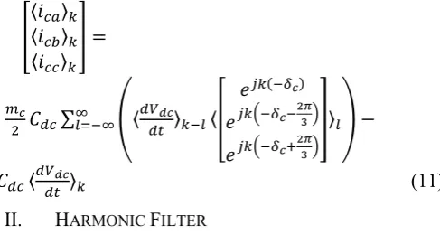
Transforming equations (8) and (9) to their equivalent dynamic phasor representations and applying equation (4) for 𝑘 harmonics yields (10) and (11).

[ 〈𝑉_𝑐𝑎〉_𝑘 〈𝑉_𝑐𝑏〉_𝑘 〈𝑉_𝑐𝑐〉_𝑘

] =

𝑚𝑐

4 ∑ (〈𝑉𝑑𝑐〉𝑘−𝑙〈[

𝑒𝑗𝑘(−𝛿𝑐)

𝑒𝑗𝑘(−𝛿𝑐−2𝜋₃)

𝑒𝑗𝑘(−𝛿𝑐+2𝜋₃)

]〉𝑙) − ∞

𝑙=−∞

𝑟_𝑐[ 〈𝑖𝑐𝑎〉𝑘

〈𝑖𝑐𝑏〉𝑘

〈𝑖𝑐𝑐〉𝑘

] −1

2〈𝑉𝑑𝑐〉𝑘 (10)

[ 〈𝑖𝑐𝑎〉𝑘

〈𝑖_𝑐𝑏〉_𝑘 〈𝑖𝑐𝑐〉𝑘

] =

𝑚𝑐

2 𝐶𝑑𝑐∑ (〈 𝑑𝑉𝑑𝑐

𝑑𝑡 〉𝑘−𝑙〈[

𝑒𝑗𝑘(−𝛿𝑐)

𝑒𝑗𝑘(−𝛿𝑐−2𝜋₃)

𝑒𝑗𝑘(−𝛿𝑐+2𝜋₃)

]〉𝑙) − ∞

𝑙=−∞

𝐶_𝑑𝑐〈𝑑𝑉𝑑𝑐

𝑑𝑡 〉𝑘 (11)

II. HARMONIC FILTER

Figure 4 represents the IDVR RLC harmonic filter. The filter output voltage, which is injected into the transformer, can be derived in three-phase form using KVL and KCL, as shown in (12) and (13).

[ 𝑉_{𝑖𝑛𝑗𝑎} 𝑉_{𝑖𝑛𝑗𝑏} 𝑉_{𝑖𝑛𝑗𝑐}] = [

𝑉𝑐𝑎

𝑉𝑐𝑏

𝑉_𝑐𝑐] − 𝐿𝑓

𝑑 𝑑𝑡[

𝑖𝑐𝑎

𝑖_𝑐𝑏 𝑖_𝑐𝑐] − 𝑟𝑓[

𝑖𝑐𝑎

𝑖_𝑐𝑏

𝑖_𝑐𝑐] (12)

[ 𝑖_{𝑖𝑛𝑗𝑎} 𝑖_{𝑖𝑛𝑗𝑏} 𝑖_{𝑖𝑛𝑗𝑐}

] = [ 𝑖_𝑐𝑎 𝑖_𝑐𝑎 𝑖𝑐𝑎

] − 𝐶_𝑓 𝑑

𝑑𝑡[

𝑉_{𝑖𝑛𝑗𝑎} 𝑉_{𝑖𝑛𝑗𝑏} 𝑉_{𝑖𝑛𝑗𝑐}

] (13)

Vinja Cf Lf Vca iinja ica icf

C rf E

Figure 4 Phasor diagram of IDVR phase ‘a’ harmonic filter

The dynamic phasor representations of equations (12) and (13) are given by (14) and (15).

[

〈𝑉𝑖𝑛𝑗𝑎〉𝑘

〈𝑉𝑖𝑛𝑗𝑏〉𝑘

〈𝑉𝑖𝑛𝑗𝑐〉𝑘

] = [ 〈𝑉𝑐𝑎〉𝑘

〈𝑉_𝑐𝑏〉_𝑘 〈𝑉𝑐𝑐〉𝑘

] − 𝐿𝑓_𝑑𝑡𝑑 [

〈𝑖𝑐𝑎〉𝑘

〈𝑖_𝑐𝑏〉_𝑘 〈𝑖𝑐𝑐〉𝑘

] −

𝑟𝑓[

〈𝑖𝑐𝑎〉𝑘

〈𝑖𝑐𝑏〉𝑘

〈𝑖𝑐𝑐〉𝑘

] − 𝑗𝜔𝐿𝑓[

〈𝑖𝑐𝑎〉𝑘

〈𝑖𝑐𝑏〉𝑘

〈𝑖𝑐𝑐〉𝑘

] (14)

[ 〈𝑖𝑖𝑛𝑗𝑎〉𝑘

〈𝑖𝑖𝑛𝑗𝑏〉𝑘

〈𝑖𝑖𝑛𝑗𝑐〉𝑘

] = [ 〈𝑖𝑐𝑎〉𝑘

〈𝑖𝑐𝑏〉𝑘

〈𝑖𝑐𝑐〉𝑘

] − 𝐶𝑓_𝑑𝑡𝑑[

〈𝑉𝑖𝑛𝑗𝑎〉𝑘

〈𝑉𝑖𝑛𝑗𝑏〉𝑘

〈𝑉𝑖𝑛𝑗𝑐〉𝑘

] −

𝑗𝜔𝐶_𝑓[

〈𝑉𝑖𝑛𝑗𝑎〉𝑘

〈𝑉𝑖𝑛𝑗𝑏〉𝑘

〈𝑉𝑖𝑛𝑗𝑐〉𝑘

4

III. SERIES INJECTION TRANSFORMER

In order to integrate more efficiently the IDVR model with the power network, the dynamic effect of the series transformer should be evaluated and included in the analysis.

For simplicity, the approximate equivalent circuit of a two-winding transformer, presented in Figure 5, is used. In this circuit the transformer inductances and resistances are lumped on the secondary side of the transformer and the magnetisation branch is neglected for the purpose of this study [11]. The three phase output voltage of the transformer is given by (16).

[ 𝑉_𝐿𝑎 𝑉𝐿𝑏

𝑉𝐿𝑐

] = 𝑇_𝑁−1_[

𝑉_{𝑝𝑐𝑐𝑎} 𝑉𝑝𝑐𝑐𝑏

𝑉𝑝𝑐𝑐𝑐

] + [ 𝑉_{𝑖𝑛𝑗𝑎} 𝑉𝑖𝑛𝑗𝑏

𝑉𝑖𝑛𝑗𝑐

] − 𝐿𝑡𝑇𝑁_𝑑𝑡𝑑[

𝐼_{𝑝𝑐𝑐𝑎} 𝐼_{𝑝𝑐𝑐𝑏} 𝐼_{𝑝𝑐𝑐𝑐}

] −

𝑟_𝑡𝑇_𝑁[ 𝐼_{𝑝𝑐𝑐𝑎} 𝐼_{𝑝𝑐𝑐𝑏} 𝐼_{𝑝𝑐𝑐𝑐}

] (16)

𝐼_𝑝𝑐𝑐 and 𝐼_𝐿 represent grid current and the load current respectively, and 𝑉_𝑝𝑐𝑐 represents the voltage at the point of common coupling (PCC).

Vpcc

Vinj

Vgrid

Vgs VLs

VL

LL _ipcc rt Lt _iL

Lo

ad

Figure 5 Phasor diagram of series injection transformer The dynamic phasor model of (16) is given by (17).

[ 〈𝑉𝐿𝑎〉𝑘

〈𝑉_𝐿𝑏〉_𝑘 〈𝑉𝐿𝑐〉𝑘

] = 𝑇_𝑁−1_[

〈𝑉𝑝𝑐𝑐𝑎〉𝑘

〈𝑉_{𝑝𝑐𝑐𝑏}〉_𝑘 〈𝑉𝑝𝑐𝑐𝑐〉𝑘

] + [

〈𝑉𝑖𝑛𝑗𝑎〉𝑘

〈𝑉_{𝑖𝑛𝑗𝑏}〉_𝑘 〈𝑉𝑖𝑛𝑗𝑐〉𝑘

] −

𝐿_𝑡𝑇_𝑁 𝑑

𝑑𝑡[

〈𝐼𝑝𝑐𝑐𝑎〉𝑘

〈𝐼_{𝑝𝑐𝑐𝑏}〉_𝑘 〈𝐼_{𝑝𝑐𝑐𝑐}〉_𝑘

] − 𝑟_𝑡𝑇_𝑁[

〈𝐼𝑝𝑐𝑐𝑎〉𝑘

〈𝐼_{𝑝𝑐𝑐𝑏}〉_𝑘 〈𝐼_{𝑝𝑐𝑐𝑐}〉_𝑘

] −

𝑗𝜔𝐿_𝑡𝑇_𝑁[

〈𝐼𝑝𝑐𝑐𝑎〉𝑘

〈𝐼_{𝑝𝑐𝑐𝑏}〉_𝑘 〈𝐼_{𝑝𝑐𝑐𝑐}〉_𝑘

] (17)

4.2 DQ DYNAMIC PHASOR MODELLING

The benefit of having models in both ABC and DQ reference frames is that each is suited to specific applications. Under balanced conditions the DQ model has some advantages, where only positive sequence components are found and where frequency variations are near to the system frequency. The DQ quantities vary more slowly than the ABC system quantities

(maximum 2-3 Hz), allowing a bigger time step and consequently faster simulation. However, the DQ model becomes inefficient when simulating system harmonics using a single reference, as the reference frame rotates at system frequency [12].

Multiplying equations (10), (11), (14), (15) and (17) by Park's transformation matrix, to transform the IDVR components to the DQ reference frame, and by applying equations (1) to (4) to obtain the dynamic phasor transformation of the IDVR equations in DQ coordinate form results in (18)-(22).

[〈𝑉_〈𝑉𝑐𝑑〉𝑘

𝑐𝑞〉𝑘] = [

∑∞𝑖=−∞〈𝑉𝑑𝑐〉𝑘−𝑖〈𝑚𝑑〉𝑖

∑∞𝑖=−∞〈𝑉𝑑𝑐〉𝑘−𝑖〈𝑚𝑞〉𝑖] − 𝑟𝑐[

〈𝑖𝑐𝑑〉𝑘

〈𝑖𝑐𝑞〉𝑘] − 1

2[〈𝑉𝑑𝑐

〉_𝑘

0 ] (18)

[〈𝑖_〈𝑖𝑐𝑑〉𝑘

𝑐𝑞〉𝑘] = 𝐶𝑑𝑐[

∑ 〈𝑑𝑉𝑑𝑐

𝑑𝑡 〉𝑘−𝑖〈𝑚𝑑〉𝑖 ∞

𝑖=−∞

∑ 〈𝑑𝑉𝑑𝑐

𝑑𝑡 〉𝑘−𝑖〈𝑚𝑞〉𝑖 ∞

𝑖=−∞

] − 𝐶_𝑑𝑐[〈𝑑𝑉𝑑𝑡𝑑𝑐〉𝑘

0 ]

(19)

[〈Vinjd〉k

〈Vinjq〉k

] = [〈V_〈Vcd〉k

cq〉k] − Lf d dt[

〈icd〉k

〈icq〉k] +

L_f [ 0_{−ω 0}ω] [〈i_〈icd〉k

cq〉k] − rf[

〈i_cd〉_k 〈i_cq〉_k]

(20)

[〈iinjd〉k

〈iinjq〉k

] = [〈i_〈icd〉k

cq〉k] − Cf d dt[

〈V_injd〉_k 〈Vinjq〉k

] +

C_f [ 0_{−ω 0}ω] [〈Vinjd〉k

〈Vinjq〉k

]

(21)

[〈VLd〉k

〈V_Lq〉_k] = TN−1[

〈Vpccd〉k

〈V_pccq〉_k] + [

〈Vinjd〉k

〈V_injq〉_k] − L_tT_N d

dt[

〈Ipccd〉k

〈I_pccq〉_k] + LtTN[ 0_{−ω 0}ω] [

〈Ipccd〉k

〈I_pccq〉_k] −

r_tT_N[〈I_〈Ipccd〉k

pccq〉k]

(22)

5. IDVR power management

Using the current direction shown in Figure 2, the DC voltage across the IDVR storage capacitor is given by (23).

𝐶_𝑑𝑐𝑑𝑉𝑑𝑐

𝑑𝑡 = 𝑖𝑑𝑐2−𝑖𝑑𝑐1 (23)

Applying a Fourier transform, the dynamic phasor transformation of (23) is given by (24).

𝐶_𝑑𝑐〈𝑑𝑉𝑑𝑐

5

between the two feeders can be measured by the total power at the DC capacitor which is equal to the difference between the ac power injected by the DC/AC converter and the ac power extracted by the AC/DC converter, as shown in (25).

𝑃_𝑑𝑐= 𝑃_𝑎𝑐2− 𝑃_𝑎𝑐1 (25) The power extracted from the second feeder is equal to the sum of the total power injected by the series transformer to the sensitive load and the active power losses in the IDVR. The upper limit of the total amount of power that can be extracted is a function of the power factor of both feeders and the total allowable voltage drop across the second feeder. Furthermore, the total power (reactive and/or active) required by the load, to compensate fault effects, depends on the compensation technique adopted for the IDVR.

6. Simulation results

The IDVR dynamic phasor model is tested using two parallel radial systems to protect a static RLC load, as shown in Figure 6 for the system parameters listed in Appendix A. In order to generate a transient condition in the distribution system, a three-phase fault is applied. The fault produces a 40% balanced voltage sag during the time interval 0.2s≤t≤0.4s and is initiated on the main feeder. The simulation is carried out for the fundamental frequency without considering harmonic effects, as mentioned in Section 3.

AC Source 15k V- 50Hz

Fault

15kV/400V

Static Load

AC Source

15k V- 50Hz Load

15kV/400V

Interline dynamic voltage restorer

PCC

Figure 6 Single-phase representation of simulated radial distribution system

The final dynamic phasor models of the IDVR in both ABC and DQ coordinate frames are constructed as modular models using converter, harmonic filter and series transformer models in conjunction with the IDVR power balance equations given in Section 5. This approach enables detailed analysis of the influence of each component of any device modelled using this technique, and provides the flexibility to test different topologies of FACTS devices with minimum modifications.

Two PI controllers are implemented in the ABC and DQ models to regulate the modulation indices and firing

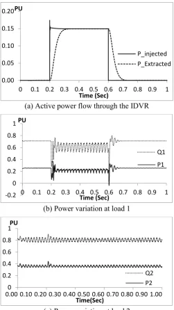
angles of both converters. While in the DC/AC converter, the aim is to control the voltage compensation and phase shift requirements, the control aim in the AC/DC converter, is to control the total active power extracted from the second feeder to maintain DC link voltage at nominal value. The fast response of the IDVR to extract and inject active power to the load is presented in Figure 7. In these three models, pre-sag compensation is applied in order to restore the pre-fault conditions of the sensitive load.

(a) Active power flow through the IDVR

(b) Power variation at load 1

(c) Power variation at load 2 Figure 7 Simulated active power flow

The IDVR dynamic phasor model successfully compensates 40% balanced voltage sag in active power injection mode and maintains the load voltage at the required value. As presented in Figure 7, the active and reactive powers of the main feeder are maintained at

0.00 0.05 0.10 0.15 0.20

0 0.1 0.2 0.3 0.4 0.5 0.6 0.7 0.8 0.9 1

PU

Time (Sec)

P_injected P_Extracted

-0.2 0 0.2 0.4 0.6 0.8 1

0 0.1 0.2 0.3 0.4 0.5 0.6 0.7 0.8 0.9 1

PU

Time (Sec)

Q1

P1

0 0.2 0.4 0.6 0.8 1

0.00 0.10 0.20 0.30 0.40 0.50 0.60 0.70 0.80 0.90 1.00

PU

Time(Sec)

6

their rated levels without affecting the powers at the second feeder. The transient appearing in the active and reactive power curves is due to the response of the circuit breaker and the IDVR model at the beginning and end of the compensation.

(a) Voltage at PCC

(b) Load current

(c) DC link voltage

(d) Load voltage

(e) Injected voltage

(f) Load Voltage of second feeder Figure 8 Simulation outputs of the IDVR dynamic

phasor model

For model verification, a comparison is carried out between the dynamic phasor model (both ABC and DQ models) and a detailed IDVR model under the same operating conditions, as shown in Figure 8. Main feeder load voltage and current, second feeder voltage, and DC link voltage are compared for the three models. As shown in the figure, the dynamic phasor models are in good agreement with the detailed model.

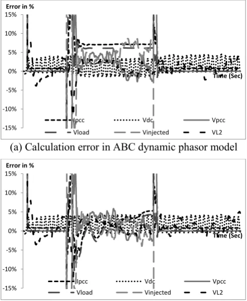
(a) Calculation error in ABC dynamic phasor model

(b) Calculation error in DQ dynamic phasor model Figure 9 Comparison of dynamic phasor model and

detailed model performance

Based on magnitude measurements from the models and the error calculation graphs of Figure 9, the differences between the ABC and DQ dynamic phasor models are less than 5% for most of the IDVR operating period, if the unstable start and end periods are ignored, and increase to 8% for the injected voltage in the ABC model for a small period of time.These results validate these two models, where a good representation of the system dynamic response rather than high-accuracy results is the requirement. These differences are a result of the approximations made during calculation of dynamic phasor models, and of neglecting harmonics in both the AC and DC components of the IDVR during the analysis. Additionally, the differences between the ABC and DQ models may be attributed to differences in controller parameter settings.

The total running times of the dynamic phasor models are much faster, at 2.9233s and 2.7939s for the

0 200 400

0.00 0.20 0.40 0.60 0.80 1.00

Volt

t(Sec)

0.0 5.0

0.00 0.20 0.40 0.60 0.80 1.00

A

t(Sec)

200 700

0.00 0.20 0.40 0.60 0.80 1.00

Volt

t(Sec)

0 200 400

0.00 0.20 0.40 0.60 0.80 1.00

Volt

t(Sec)

0 200 400

0.00 0.20 0.40 0.60 0.80 1.00

Volt

t(Sec)

0 200 400

0.00 0.20 0.40 0.60 0.80 1.00

Volt

t(Sec)

-15% -10% -5% 0% 5% 10% 15%

Error in %

Time (Sec)

Ipcc Vdc Vpcc

Vload Vinjected VL2

-15% -10% -5% 0% 5% 10% 15%

Error in %

Time (Sec)

Ipcc Vdc Vpcc

Vload Vinjected VL2

Detailed DQ-Dynamic ABC-Dynamic

Detailed DQ-Dynamic ABC-Dynamic

Detailed DQ-Dynamic ABC-Dynamic Detailed DQ-Dynamic ABC-Dynamic

Detailed DQ-Dynamic ABC-Dynamic

7

ABC and DQ dynamic phasor models respectively, when compared to that of the detailed model, which is 7.5667s, when simulating 1s of IDVR operation using the same computer.

7. Conclusion

A dynamic phasor model of interline dynamic voltage restorer (IDVR) has been proposed based on modular representation of its components including power converter, filter stage and series injection transformer. This has enabled more detailed illustration of the effects of individual components and parameters on IDVR operation, and simple construction and modelling of different topologies. The IDVR was modelled and analysed in both ABC and DQ coordinate frames, and was simulated using MATLAB/Simulink. The benefit of having two models in the ABC and DQ reference frames is the suitability of each model under different balanced and unbalanced conditions.

The outputs from the dynamic phasor models are in good agreement (typically within 5%) with those from the detailed model as shown in the simulation results and the error calculation graphs.

In addition, the time required to simulate the dynamic phasor models was shown to be less than 50% of that required for the detailed model, whilst maintaining the dynamic behaviour of the device.

The dynamic phasor modelling technique enables accurate results and fast simulation time even for complex systems, with acceptable calculation errors. Possible applications of dynamic phasor modelling are transient stability programs and other real-time simulations that require such fast simulation models. In addition, constructing models using modular modelling techniques provides a common base for different FACTS devices and power system components in the simulation library for future applications and topologies.

Appendix A

Main source: 15kV, 50Hz

Transformer: 3Ø ∆∆, 10kVA, 15kV/400V Load: 3Ø static load, P=3kW, Q=3kVAr Initial DC capacitor voltage = 650V DC capacitance = 7200µF

Switch resistance = 1mΩ

Filter R = 1Ω, L = 60mH and C = 75µF Series transformer R = 0.385Ω and L = 0.963H

Bibliography

[1] S. Chiniforoosh, J. Jatskevich, A. Yazdani, V. Sood, V. Dinavahi, J. A. Martinez, et al., "Definitions and Applications of Dynamic Average Models for Analysis of Power Systems," IEEE Transactions on Power Delivery, 2010.vol. 25, pp. 2655-2669.

[2] Z. E, K. W. K. Chan, and D. Fang, "Dynamic phasor modelling of TCR based FACTS devices for high speed power system fast transients simulation," Asian power electronics journal, vol. 1, pp. 42-48, Aug-2007.

[3] A. M. Stankovic and T. Aydin, "Analysis of asymmetrical faults in power systems using dynamic phasors," IEEE Transactions on Power Systems, vol. 15, pp. 1062-1068, 2000.

[4] S. Yao, M. Bao, Y. n. Hu, M. Han, J. Hou, and L. Wan, "Modeling for VSC-HVDC electromechanical transient based on dynamic phasor method," 2nd IET in Renewable Power Generation Conference (RPG 2013), 2013, pp. 1-4.

[5] H. Zhu, Z. Cai, H. Liu, and Y. Ni, "Multi-infeed HVDC/AC power system modeling and analysis with dynamic phasor application," IEEE/PES Transmission and Distribution Conference and Exhibition: Asia and Pacific, 2005, Aug. 2005, pp. 1-6.

[6] W. Yao, J. Wen, H. He, and S. Cheng, "Modeling and simulation of VSC-HVDC with dynamic phasors," Third International Conference on Electric Utility Deregulation and Restructuring and Power Technologies (DRPT2008), 2008. pp. 1416-1421.

[7] T. Demiray, F. Milano, and G. Andersson, "Dynamic phasor modeling of the doubly-fed induction generator under unbalanced conditions,"Power Tech, 2007 IEEE Lausanne, 2007, pp. 1049-1054.

[8] D. M. Vilathgamuwa, H. M. Wijekoon, and S. S. Choi, "Interline dynamic voltage restorer: a novel and economical approach for multi-line power quality compensation," Conference Record of the Industry Applications Conference, 38th IAS Annual Meeting, 2003.pp. 833-840 vol.2.

[9] M. A. Hannan, A. Mohamed, and A. Hussain, "Dynamic Phasor Modeling and EMT Simulation of USSC,",Proceedings of

the World Congress on Engineering and Computer Science, WCECS. San Francisco, USA. 2009. pp. 20-22.

[10] A. Nabavi-Niaki and M. R. Iravani, "Steady-state and dynamic models of unified power flow controller (UPFC) for power system studies," Power Systems, IEEE Transactions on, 1996, vol. 11, pp. 1937-1943.

8