Using the scaled boundary finite element method to model 2D time-dependent geotechnical engineering problems

Using the scaled boundary finite element method to model 2D time-dependent

geotechnical engineering problems

A. El-Hamalawi

1

& M. Hassanen

2

1 _{Civil & Building Engineering Department, Loughborough University, United Kingdom}

[email protected]

2 _{Civil Engineering Department, University of Strathclyde, John Anderson Building, 107 Rottenrow,} Glasgow G4 ONG, United Kingdom

[email protected]

ABSTRACT. The scaled boundary finite element method caters well for soil-structure interaction problems, but the formulation does not cater for the presence of changing pore pressures with time, body loads and tractions. A detailed formulation is presented in this paper to consider the general 2D analysis case for modelling coupled consolidation, accounting for body forces and surface tractions in both the bounded and unbounded media. The advantages of this method compared to conventional methods are also explained in this paper.

1. Introduction

In general, the current methods used to numerically model the unbounded far-field boundary in dynamic soil-structure interaction problems truncate the remote boundaries and then impose free or fixed boundary conditions. If input waves originate at the structure and propagate through the soil towards infinity, the artificial far-field domain boundary would reflect waves back into the near-field and structure, thus producing erroneous results. Several methods of circumventing this have been used but are either restricted to very simple cases, or involve too many approximations. The recently developed scaled boundary finite element method (Song and Wolf, [2]) achieves an accurate representation as the radiation boundary condition at infinity is satisfied exactly. This however only exists for a single-phase medium, and very recently two-phase medium with no body loads, and is thus not applicable to a wide range of practical geotechnical problems, where the medium modelled is a two-phase fully saturated soil and the body forces are nearly always present. The method combines many advantages of both the finite-element and boundary-element methods, while avoiding many of their disadvantages. For example, unlike the boundary-element method, the scaled boundary finite element method does not require a complex fundamental solution or encounters singular integrals. A reduction of the spatial dimensions by one is also achieved (Song and Wolf, [3]). Moreover, among the advantages of the scaled boundary finite element method (which is a semi-analytical fundamental-solution-less boundary-element method based on finite elements) is the non-discretisation of the free surfaces, or between material interfaces. The full scaled boundary finite element method is covered comprehensively by Wolf and Song [4]. Wolf and Hout [5] recently extended the method to two-phase media but assumed no body forces and omitted the surface tractions. The aim of this paper is to formulate the ordinary differential equations for the two-phase media considering the body forces and including the surface tractions.

2. The Governing Equations

The coupled consolidation equations, developed by Biot [1], comprise a system of simultaneous differential equations which satisfy; (a) the equilibrium conditions (the dynamic equations of motion) and (b) the continuity equations. The 2D form of these equations in the frequency domain are shown as equations (1a) and (1b).

[ ] { } { }

LT

(

σ′ + m p

)

+ω2ρ

{ } { }

u +ρ b =0 (1a)

{ }

[ ][ ] { }

+ 2

{ }

[ ]{ }

+

{ }

[ ]{ }

+

{ }

[ ]{ }

+ =0

− p

K n i u L m i b L m k u L m k p m L L m k

f T

T f T

f T

T _{ω ρ ρ ω ω}

The differential operator

[ ]

L is defined by equation (2)

.

σ

′

is the effective stress, is the fluid pressure (in which the total stress

p

σ relates to the fluid pressure by

{ } { } { }

σ = σ′ + m p), u, ω, k, n, Kf

and ρ are the displacement, frequency, soil permeability and porosity, fluid bulk modulus and density respectively, and

{ }

b is a vector representing the body forces per unit volume.

[ ]

L 0x 0

y x

∂ ∂

y

 

 

=_ ∂ ∂ _

∂ ∂ ∂ ∂ 

 

(2)

3. Scaled Boundary Transformation of Geometry

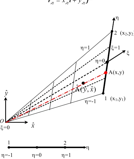
Consider a finite line element 1-2 forming the base of the triangle shown in Fig. 1. Any point A on the boundary line element 1-2, with local coordinates , can be represented by its position vector

(x, y)

r, where . If the origin,

O

, of the Cartesian coordinates coincides with the apex of the triangle, then a point within the domain may be described in the Cartesian coordinates by its global position vector as r

j i

r=x + y (x, y)ˆ ˆ

r

ˆ

ˆ=xˆi+yˆj. To transfer from the Cartesian to the curvilinear co-ordinate system ( ,ξ η), any point within the domain (in which

ξ

=1 at the boundary and

ξ

=0 at the scaling centre) may be described by scaling using the position vector of the corresponding boundary point;

r

ˆ

=

ξ

r

_{. Fig. 1 shows the geometry of the line boundary with the tangential vector}

(slope) in the

η

direction, represented by the derivative of the point A’s position vector on the line as shown in equation (3) :

j i

r_,η =x_,η +y_,η (3)

1 (x1,y1)

2 (x2,y2)

ξ=1 ξ η=1

η=-1

ξ=0

O

η

η=0

A(x,y)

η

η=-1 η=0 η=1

1 2

) ˆ , ˆ ( Aˆ y x yˆ

[image:2.595.174.394.418.680.2]

xˆ

FIGURE 1. Scaled boundary transformation of geometry of line finite element

Mathematically, the geometry of the boundary of the finite element shown in Fig. 1 may be represented by interpolating its nodal coordinates

{ }

x

and

{ }

y

using the local coordinates

η

at the boundary as follows :

[

N

]

{ }

x

[ ]

N

{ }

x

where

[ ] [

N = N(η,ζ)

] [

= N₁(η,ζ) N₂(η,ζ) .. .. N_n(η,ζ)

] [

= N₁ N₂ .. .. N_n

]

and is the number of element nodes. Using the scaling relationship

n

r

rˆ=ξ to describe the position of any point within the domain leads to

) ( ) , (

ˆ ξ η ξxη

x = and yˆ(ξ,η)=ξy(η) (5)

Equation (6) is used to transfer the differential operators in the (x co-ordinate system to those corresponding to the ( , co-ordinate system.

ˆ ˆ, y) )

ξ η

1

, ,

x _{ˆJ( , )} 1 y x

y J y x

− _{η η}

∂ ∂ ∂ ∂ξ − ∂ ∂ξ

  _{ }     

= ξ η =

_{∂ ∂}  _{ } _{∂ ∂η} _{− } _{ξ∂ ∂η}

      1

  

)

) (6)

where the Jacobian matrix is

[

]

_and the determinant is

  

  =

η η

ξ ξ

η ξ

, ,

, ,

ˆ ˆ

ˆ ˆ ) , ( ˆ

y x

y x

J J =xy,η −yx,η. At ξ =1, on

the curved boundary, the outward normal vector is defined by equation (7).

j i r

g ,η η η

ξ

, , x

y −

=

= (7a)

The unit normal vector, nξ is thus

] [

1

, , i j

j i g

n _ξ ξ ξ _{ξ η η}

ξ ξ

x y g n n

g = x + y = −

= (7b)

Similarly, the outward normal vector to the line ( )ξ is gη:

j i r

gη = =−y +x (8a)

and the corresponding unit normal vector is nη.

] [

1

j i j

i g

n y x

g n n

g = x + y = − +

= η η _η

η η η

(8b)

where 2

, 2

, ) ( )

( η η

ξ ξ

x y

g = g = + − _and gη = gη = (−y)2+(x)2 . Substituting the derivative relationships results in :

   

 

   

 

∂ ∂ ∂

∂ ∂

∂ ∂

∂ =

     

     

∂ ∂ ∂

∂

    

   =      

     

∂ ∂ ∂

∂

η ξ

ξ

η ξ

ξ

η ξ

ξ

η η ξ

ξ

η η ξ

ξ

η η ξ ξ

η η ξ ξ

y y

x x

y y

x x

n g n

g

n g n

g

J n

g n g

n g n g

J y x

1 1 1

1 1

ˆ

)

(9)

Substituting equation (9) into the differential operator

[ ]

L in equation (2) results in equation (10).

[ ]

x x

x x

1 2

y y y y

y x y x

y y x x

1

g n g n 0

n 0 n 0

1 1 g g

L 0 g n g n 0 n 0 n b

J J J

n n n n

1 1

g n g n g n g n

ξ ξ η η

ξ η

ξ η

ξ ξ η η ξ η

ξ ξ η η

ξ ξ η η ξ ξ η η

 ∂ ∂ 

+

 _{∂ξ ξ ∂η} 

     

 ∂ ∂    ∂   ∂ _{ } ∂ _{ }

= _ + _= _{ } + _{ } =_{   }

∂ξ ξ ∂η ∂ξ ξ ∂η ∂ξ ξ ∂η

  _ _ _ _

 ∂ ₊ ∂ ∂ ₊ ∂ 

 _{∂ξ ξ ∂η ∂ξ ξ ∂η}

 

1

b ∂

where

x , x

1 2

y , y

y x , , y x

n 0 y 0 n 0 y 0

g 1 g 1

b 0 n 0 x , b 0 n 0 x

J J J J

n n x y n n x y

ξ η

η

ξ η

ξ

η

ξ ξ η η

η η

      −

η

 

       

 = _{ }= −  = _{ }=

       

  _− _   _ − _

   

. It should be noted that

the transpose of the differential operator,

[ ]

L T, may be expressed as

[ ]

[ ]

[ ]

η ξ

ξ ∂

∂ +

∂ ∂

= T T

T

b b

L 1 1 2 _.

Applying the transformation in equation (9) to the differential motion and continuity equations yields

[ ]

{ }

1

[ ]

{ }

[ ]

{ }

1

[ ]

{ }

2

{ } { }

0

, 2

, 1

, 2 ,

1 ′ + _b ′ + _{b m p} + _{b m p} + _u + _b =

b T T T T ω ρ ρ

ξ σ

ξ

σ_{ξ η ξ η (11)}

{ }

[ ] [ ]

[ ]

[ ] [ ]

[ ]

{ }

{ }

[ ]

{ }

[ ]

{ }

{ }

[ ]

{ }

[ ]

{ }

{ }

(

[ ]

{ }

1

[ ]

{ }

) 0

) 1

( )

1 (

)) 1

( 1

) 1

( (

, 2 ,

1

, 2 ,

1 ,

2 ,

1 2

2 1

2 2

1 1

= +

+ +

+ +

+ +

∂ ∂ +

∂ ∂ ∂

∂ +

∂ ∂ +

∂ ∂ ∂

∂ −

p K

n i u b u

b m i

b b b

b m k u b u

b m k

p m b

b b

b b

b m k

f T

T f T

f

T T

T T

T

ω ξ

ω

ξ ρ

ξ ρ

ω

η ξ

ξ η

ξ η ξ

ξ ξ

η ξ

η ξ

η

ξ (12)

4. Displacements and pore pressure shape functions

Shape functions similar to the mapping interpolation functions may be used to interpolate the finite element displacements for all lines with constant ξ. Using displacement shape functions

[

Nu(η)

]

and displacements functions in the radial direction

{ }

u(ξ) , the finite element displacement function may be represented as

{ } {

}

u

{

}

u

u = u( , , )ξ η ζ =_N _ u( ) where Nξ _  _{ }= N ( , )u η ζ _ (13a)

and hence

{ }

{

}

{ }

{

}

{ }

{

}

u u

, _, , _, ,

uξ =N  u( )ξ ξ , uη =N η u( ) and uξ ζ =N  u( )

u

,ζ ξ (13b)

Similarly, the pore pressure function may be represented using the shape functions

[

Np(η,ζ)

]

and pressure functions in the radial direction

{

p(ξ)

}

. Hence the finite element pore pressure function may be represented as

{

p(ξ,η)

}

[ ]

N

{

p(ξ)

}

p= p where

[ ] [

Np = Np(η)

]

(14a)

and hence p,ξ

[ ]

N

{

p(ξ)

}

,ξ

p

=

where

p

{

}

p

{

}

p

{

}

p

{

}

, _, , _, , _, , , _{, ,}

pη=N η p( ) , pξ ξξ=N  p( )ξ ξξ , pηη=N ηη p( ) and pξ ξη=pηξ =N η p( )ξ ξ

(14b)

The stresses, strains and displacements are related by

{ }

σ =′

[ ]

_D

{ }

ε =

[ ][ ]

_{D L u}

{ }

=

[ ][ ]

_{D L} _Nu

{

_u(ξ

}

  ) (15)

where

[

D

]

is the constitutive matrix and

[ ]

[ ]

[ ]

[ ]

ζ ξ η ξ

ξ ∂

∂ +

∂ ∂ +

∂ ∂

= 1 1 2 1 3

b b

b

L . This leads to

{ }

[ ]

1

{ }

2

{ }

3

{ }

[ ]

1 u

{ }

(

2 u 3 u

)

{ }

, , , _,

, ,

1 1 1

D b uξ b uη b uζ D b N u( ) ξ b N η b N ζ u( )

  

′                  

σ = _{ } + _{ } + _{  }= _{   } ξ + _{   } +_{   } ξ

ξ ξ ξ

  

which can be expressed as

{ }

[ ]

[ ]

{

}

[ ]

{

}

_      ₊ =

′ ( ) 1 2 ( )

,

1 ξ

ξ ξ

σ D B_u u _ξ B_u u (17)

where 1 1 u 1 u 2 2 u 2 u

u u _{, ,}

B b N ( ) b N and B b N ( ) _η b N _η

    = η =         = η =  

                    . Note that

[ ]

B

u1 and

[ ]

2

u

B

are not dependent on ξ, and hence differentiating

{ }

σ′ leads to

{ }

[ ]

[ ]

{ }

[ ]

{ }

[ ]

{ }

_      − + =

′ ( ) 1 ( ) 1 2 ( )

2 , 2 ,

1

, ξ _ξ ξ _ξ ξ

σξ D B u ξξ B u ξ B u (18)

5. Weighted-residual finite element approximation

To derive the finite element approximation, the Galerkin’s weighted-residual method is applied to the transformed differential equations of motion and continuity, equations (11) and (12), by multiplying them with a weighting function

{ }

T

{

}

T

w

w = (ξ,η) and then integrating over the domain

. Integration is from –1 to +1 for the boundary variable

A η while the integration in the

ξ

direction is from 0 to +1 for bounded elements and from +1 to ∞ for unbounded elements.

The weighting function

{

to be multiplied by the differential equation of motion can be represented by the same displacement function as

}

T u

w

{ }

u

{

u

( )

ξ η

}

[

u

( )

η

]

{

u

( )

ξ

}

w w

w = , = N _{. The weighting}

function

{

to be multiplied by the differential equation of continuity, in turn, can be represented by the same pore pressure function as

}

T

wP

{ }

{

( )

η

}

[

P

( )

η

]

{

P

( )

ξ

}

N

, = w

ξ

P P

w

w = . Green’s theorem is finally applied to theline integral. The final equations are shown in Section 6.

6. Summary of the Finite Element Coupled Consolidation Equations

Due to the space restrictions, only the final formulation of the finite element derivation is presented in the form of equations

[ ]

{

}

[ ] [ ] [ ]

{

}

[ ]

{

}

[ ]

{

}

[ ]

{

}

[ ] [ ]

)

{

( )

}

{

( )

} {

( )

}

0 ( ) ( ) ( ) ( ) ( ) ( ) ( 2 4 3 , 2 3 2 0 2 2 , 1 1 0 , 2 0 = + + − + + + − + − + ξ ξ ξ ξ ξ ξ ξ ξ ξ ξ ω ξ ξ ξ ξ

ξ ξξ ξ ξ

t b T F F p E E p E u M u E u E E E u E (19)

[ ]

{

}

[ ] [ ] [ ]

{ }

{

}

[ ]

{ }

{

}

[ ]

{

}

[ ]

{ }

[ ] [ ]

{ }

{ }

{

}

{

( )

} {

( )

} {

( )

}

0

) ( ) ( ) ( ) ( ) ( ) ( ) ( ) ( ) (

)

(

)

(

)

(

)

(

4 3 2 1 2 3 4 3 2 , 2 3 2 2 1 2 7 , 1 6 6 5 , 2 5 = + − + − + − + − + − − + − + + + − + ξ ξ ξ ξ ξ ξ ξ ξ ρ ξ ξ ρ ω ω ξ ξ ρ ω ω ξ ξ ω ξ ξ ξ ξ ξ ξ ξ ξξ b b b b f t P T f T f t t T F F F F k u F E E k i u E k i p M i p F E p F E E E p E (20) where

[ ] [ ]

+

_∫

[ ]

[ ]

− = 1 1 1 1

0 _{B D B Jd}η

E _u T _u

[ ] [ ]

∫

[ ]

[ ]

+ − = 1 1 1 2

1 _{B D B Jd}η

E _u T _u

[ ] [ ]

∫

[ ]

[ ]

+ − = 1 1 2 2 2 η d J B D B

E _u T _u

[ ] [ ]

+

_∫

{ }

[ ]

− = 1 1 1 3 η d J N m B

E T p

u

[ ] [ ]

∫

{ }

[ ]

+ − = 1 1 2 4 η d J N m B

E T p

u

[ ] [ ] [ ]

E B N Jdη

u T p P

∫

+ − = 1 1 2 4

[ ] [ ] [ ]

+

_∫

− = 1 1 1 1 5 η d J B k B E p T

p

[ ] [ ] [ ]

∫

+ − = 1 1 1 2

6 _{B k B Jd}η

E _p T _p

[ ] [ ] [ ]

∫

+ − = 1 1 2 2

7 _{B k B Jd}η

[ ] [ ] [ ]

+

_∫

−

= 1

1

0 _N ρ _{N Jd}η

M u T u

[ ] [ ]

[ ]

∫

+

−

= 1

1

1 _{N Jd}η

K n N

M p

f T p

{

}

+

_∫

[ ]

{ }

−

= 1

1

)

(ξ N ρ b Jdη

Fb u T

{

}

(

[ ]

{ }

)

1 1

) ( )

(

+

−

= η _ξ η

ξ N t g

Ft u T

{ }

(

[ ] [ ]

)

1

1 1 2

1 +

−

= B k B J

F p

T A p t

{ }

(

[ ] [ ]

)

1 1 2 2

2 +

−

= B kB J

F p

T A p

t

{ }

(

[ ] [ ]

)

1

1 2

3 +

−

= B N J

F A T u

p

t

{

}

[ ]

{ }

∫

+

−

= 1

1 , 1 1

)

(ξ B bξ Jdη

Fb _p T

{

}

+

_∫

[ ]

{ }

−

= 1

1 1 2

)

(ξ B b Jdη

Fb _p T

{

}

∫

[ ]

{ }

+

−

= 1

1 2 3

)

(ξ B b Jdη

Fb _p T

{

}

(

[ ]

{ }

)

1 1 2

4_{( )} +

−

= B b J

F A T

p b ξ

[ ] [ ][

u

] [ ][ ]

u

u b N b N

B1 = 1 (η) = 1

[ ] [ ][

η

] [ ][ ]

η ,η

2 , 2

2

)

( u

u

u b N b N

B = =

[ ] [ ]

T

{ }

[

p

] [ ]

T

{ }

[ ]

p

p b m N b m N

B1 = 1 (η) = 1

[ ] [ ]

B_p2 = b2 T

{ }

m

[

Np(η)

] [ ]

_,η = b2 T

{ }

m

[ ]

Np _,η

[ ] [

2

]

{ }

[ ] [ ]

2

{ }

[ ]

2

)

( m b N m b

N

BpAT = p η T T = p T T

6. Conclusion

A numerical formulation to correctly model the dynamic unbounded far-field boundary for two-phase media has been developed. The method of analysis extends the existing single-two-phase scaled boundary finite element method into a two-phase coupled solid-fluid approach to produce a more realistic representation of saturated soil at the unbounded far-field boundary. Body forces and surface tractions are considered in the derivation. The concept of similarity, the compatibility equation and Biot’s coupled consolidation equations have been used to derive the formulation for the governing equations. The main difference from the single-phase version is the presence of pore water pressures as additional parameters to be solved for, in addition to the displacements, strain and stress. These are incorporated into the static-stiffness matrices by producing fully coupled matrices. Solving the resulting equations yields a boundary condition satisfying the far-field radiation condition exactly. The computed solutions are exact in a radial direction (perpendicular to the boundary and pointing towards infinity), while converge to the exact solution in the finite element sense in the circumferential direction parallel to the soil-structure boundary interface.

7. References

[1] Biot, M. A., General theory of three-dimensional consolidation, Journal of Applied Physics, 12, 1941, 155-164.

[2] Song C., Wolf J. P., Consistent Infinitesimal finite-element-cell method: out-of-plane motion, The scaled boundary finite-element in the frequency domain. ASCE Journal of Engineering Mechanics, 121, 1995, 613-619.

[3] Song C., Wolf J. P., The scaled boundary finite-element in the frequency domain. Computer Methods in Applied Mechanics and Engineering, 164, 1998, 249-264.

[4] Wolf J. P., Song C., Finite Element Modelling of Unbounded Media. John Wiley and Sons, New York (1996).