Verification of damage ship survivability with computational fluid dynamics

Verification of damage ship survivability with computational

fluid dynamics

Athanasios Niotis,MSRC, NAOME, Glasgow, [email protected] Dracos Vassalos,MSRC, NAOME, Glasgow, [email protected]

Evangelos Boulougouris,MSRC, NAOME, Glasgow, [email protected] Jakub Cichowicz,MSRC, NAOME, Glasgow, [email protected]

Georgios Atzampos,MSRC, NAOME, Glasgow, [email protected] Donald Paterson,MSRC, NAOME, Glasgow, [email protected]

ABSTRACT

In the new era of direct stability assessment (DSA) for ship survivability in intact and damaged conditions, direct and accurate evaluation of the safety level achieved by the design plays a vital role. Two are the most popular methods for DSA namely, time domain numerical simulation (TDNS) and Computational Fluid Dynamics (CFD). Both can be used for the evaluation of the safety level of a ship post casualties, following collision or a grounding incidents. It is common practice for the TDNS methods to have as a core a hydraulic model for capturing the propagation of the floodwater and its dynamics in order to reduce the computational cost. However, more recently, CFD methods have matured enough to provide a credible alternative, particularly concerning the investigation of complex fluid dynamics problems. The catch, however, is higher computation costs and this is where ingenuity helps. This paper proposes and demonstrates the feasibility of using high fidelity computational fluid dynamics tools for direct damage stability assessment of ships.

Keywords: damaged ship, numerical tank, survivability verification, CFD, OpenFOAM.

1. INTRODUCTION

The survivability of a ship after damage has been in the forefront of interest of the maritime community for almost six decades. Accidents of the past with devastating consequences in terms of human loses, environmental damage and financial cost have raised the alarm in the area of maritime safety. Engineers and scientist have been trying to investigate this complex hydrodynamic challenge using as main tools model experiments and numerical simulations.

Until the 1980s, the primary way to investigate the behaviour of a ship after damage was by model testing. However, limitations such as facility availability, cost, time, and physical constraints (e.g., scale effects and dynamic similarity) encouraged the development of mathematical models and numerical tools, which capture the physics accurately and to study allow to study the problem by means of numerical simulations.

Time domain simulation of flooding after damage is a very intriguing theoretical and

engineering challenge, which started being investigating numerically since the 1980s at the University of Strathclyde in Glasgow. The main difficulty in this inquiry stems from the coupled non-linear dynamics between ship and floodwater, with complex interactions between ship, floodwater and environmental conditions.

and Spanos introduced a lumped-mass model for the simulation of the floodwater dynamics inside the damaged compartment (Zaraphonitis, Papanikolaou, & Spanos, 1997; Spanos & Papanikolaou, 2001; Papanikolaou & Spanos, 2002). Santos & Soares, in 2006 used shallow water equations for the modelling of the floodwater behaviour. Ruponen, in 2007, developed a pressure correction technique based on the hydraulic model assumptions for the floodwater propagation in the internal spaces of the ship, which is represented as a hydraulic network.

The majority of the methods, which have been proposed are based on coupling hydraulic models for the floodwater propagation with quasi-static or dynamic models. Furthermore, the equations of ship motions are often linearized and based on the impulse response technique for transforming the results of the potential flow frequency domain to the time domain (Cummins, 1962). The fundamental assumptions of these models and the complexity of the phenomenon in question still leave some uncertainties regarding the capturing of its crucial characteristics, especially in the transient phase of flooding, which can profoundly influence the survivability of ships after damage (Vassalos, et al, 2003).

On the other hand, the astonishing theoretical and technological advancements in the field of CFD allowed researchers to use grid based RANS solvers or mesh free CFD techniques for the simulation of flooding of a ship after damage (van't Veer & de Kat, 2000; Strasser, Jasinowski, & Vassalos, 2009; Sadat-Hosseini, et al., 2012; Gao, Vassalos, & Gao, 2010; Shen & Vassalos, 2011; Skaar & Vassalos, 2006). However, their complexity and computational cost rendered the systematic use in a more systematic manner infeasible.

This work attempts to demonstrate the utilisation of CFD techniques for direct damage stability assessment and the survivability of ships after damage. Furthermore, it discusses challenges, limitations and opportunities in the direct comparison between high fidelity numerical fluid dynamic algorithms and time-domain simulation tools in the problem at hand.

2. TIME-DOMAIN SIMULATION

The time-domain simulation software, which has been used in this work is PROTEUS3 (Jasionowski, 2001).

The three main elements in the time-domain simulation of the motion of a ship after damage are the mathematical description of ship motion, the floodwater ingress and dynamics, and the environmental conditions, which influence the behaviour of both ship and floodwater.

Ship Dynamics

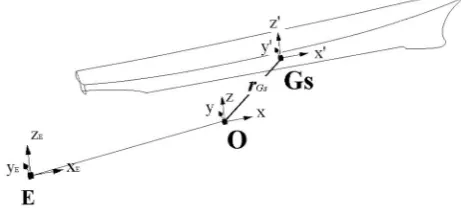
The mathematical description of ship motions is based on six degree of freedom rigid body motion equations, which derive from the conservation of linear and angular momentum.

Figure 1: The coordinate systems used in the analysis.

The modelling of rigid body dynamics, involves three coordinate systems. An earth-fixed inertial frame of reference is assumed in point E with axes . The second, inertial reference system has its origin at point (usually placed at the intersection of the midship section, with the centre line plane and the waterline plane of the intact vessel at calm sea), local axis and it moves with the average velocity of the hull.

The equations of motion of the ship are solved based on a third reference system attached to the centre of gravity of the intact vessel.

The motions of the ship are described by two vector equations, derived from the conservation of linear and angular momentum respectively (Jasionowski, 2001).

= (1)

= (2)

Where, and are the external forces and moments acting on the body in respect to the Oxyz frame of reference. The linear momentum of the translating body and the angular momentum relative to the same coordinate system are

= × ∙ (4)

Where is the finite mass of the rigid body, its velocity and its position vector with respect to the

.

The total mass of the vessel in each time instant is the sum of the intact ship mass and the total floodwater mass , which is equal with the addition of the floodwater mass in each individual compartment ,∑ .

= + = + ₍₅₎

Assuming that the floodwater mass in each compartment is concentrated to its centre of gravity the equations (3) and (4) are equal with

= ∙ + ∙ (6)

= × ∙ + × ∙ (7)

where, , the position and velocity vectors of the centre of gravity of the intact ship mass with respect to the coordinate system, and ,

the position and velocity vectors of the centre of gravity of each floodwater mass in respect to the same coordinate system.

The final equations of linear and angular momentum equations as derived form the (6) , (7) after the trnasformation of the frame of reference form the to the are (Jasionowski, 2001),

∙ + 2∙ ×

+ ∙ × +

×( × )

+ ∙ ( + × ) (8)

+( + ) ∙ + ∙ +

×( + ) ∙ =

( + ) ∙ + ∙ ×

+ ∙ [( × )× ]+ ∙

+ ∙ × + ×( + ) (9)

+ ∙ [ ×( + )]

+ × ( + ) ∙ =

In the equations (8) and (6) the force and the momentum and are calculated in the body fixed

reference system .

The external forces and moments are determined based on the supposition of the following hydrostatic and hydrodynamic entities: Froude-Krylov forces calculated with body exact formulation; radiation and diffraction forces calculated in the frequency domain using linear potential theory and then transferred to time domain with the incorporation of convolution and spectral techniques (Vassalos D. , 2014). These forces pre – calculated for a range of loading conditions, speed and headings; and the values are stored in a hydrodynamic database. During the time-domain simulations the instantaneous values interpolated from the database.

Floodwater ingress

The floodwater ingress and propagation use hydraulic models. The volumetric flow rate is calculated, based on the Bernoulli equations as a function of the difference of the hydrostatic heads ℎ between sea and damaged compartment (Vassalos, Turan, & Pawlowski, 1997).

= ∙ ∙ 2∙ ∙ ℎ ∙ (10)

Where, is a pressure loss coefficient, the effective area of the opening and the accelleration of gravity.

3. CFD FOR FLOODING SIMULATION

specific issues that simplified time-domain simulation models cannot capture.

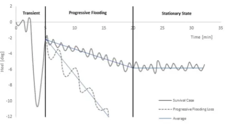
The flooding process after collision or grounding can be divided into three stages: transient, progressive flooding, and stationary-state (Vassalos, Jasionowski, & Guarin, 2006; Jasionowski, Vassalos, & Guarian, 2004). The peculiarity of this problem is that each stage requires a different level of detail in its physical modelling.

Figure 2: Flooding stages of a ship after damage.

CFD for transient flooding

When a ship or floating structure suffers from a breach on her hull, the very first moment of the incident is characterised by the complex hydrodynamics equilibrium. The pressure gradient in the vicinity of the damage opening prompts the generation of a high momentum fluid jet. The accurate capturing of the impact of the jet is vital for the assessment of the survivability of the vessel in transient response. The momentum of the jet is influenced by the hydrodynamic pressure at the opening, the geometry of the damage and the internal arrangement that receives the impacting jet. High fidelity CFD tools can provide critical insight into the complex hydrodynamics of this stage that simplified hydraulic models cannot capture.

CFD for progressive flooding

The next stage of the flooding process is the propagation of the floodwater in the vicinity of the damaged compartments through internal openings. The course of this stage is highly influenced by the watertight and non-watertight subdivision of the vessel as well as the sea condition. The problem can be closer to a hydraulic network routing in case of ships with a complex arrangement such as cruise ships or a hydrodynamic nature in the case of ships with large undivided spaces, such as the car deck of RoPax vessels. A key element for the accurate

prediction of the survivability of the ship, during this stage, is her response to waves. In the final stages of the progressive flooding and before the stationary state condition the fast, simplified models have an advantage as the nature of the problem is driven largely by hydraulic energy rather than the hydrodynamic momentum. Still, CFD models can give a better insight into the impact of various design details, which influence the outcome of the incident. Examples include the collapse of watertight doors, the influence of the arrangement of the openings, and a better prediction of the motions of the vessel under various environmental conditions.

4. LIFE-CYCLE FLOODING RISK

ASSESSMENT FRAMEWORK

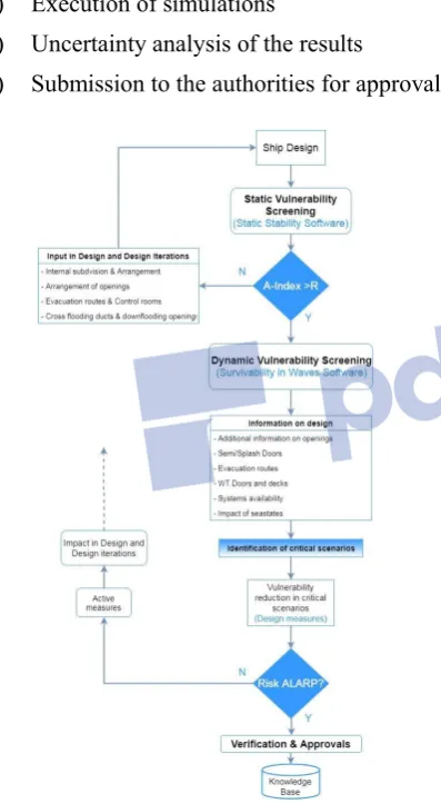
The Life-Cycle Flooding Risk Assessment Framework introduces a coherent decision-making rationale for the evaluation of the safety level of a ship against flooding. This approach entails the survivability assessment of the ship after flooding during the design phase, the operational phase and the emergency response phase, each of them having deferent safety objectives and employs different tools (Vassalos, et al., 2018).

A primary characteristic of this approach is that it evolves as the design and the operation of the vessel unfolds. The initial stage of the design starts with static vulnerability assessment and as the design process unfolds and becomes more detailed the assessment changes in nature and becomes dynamic with the use of time-domain simulation tools. The assessment finally is verified with the incorporation of CFD tools, which are used for vulnerability assessment and verification in critical scenarios.

Static Vulnerability Screening (SVS)

The static vulnerability screening stage includes the probabilistic damage calculations based on the current SOLAS accident statistics. The output from this stage is the most critical scenarios which pass to the next stage of the dynamic vulnerability screening. The demarcation of the critical cases is based on the hydrostatic properties at the equilibrium position as it judged by the SOLAS regulations.

Dynamic Vulnerability Screening (DVS)

various operating and environmental conditions. The identified vulnerabilities can be either limited by design solutions or watertight door management and damage control options.

Verification & Approval (V&A)

This stage incorporates the use of a numerical wave tank based on high fidelity CFD tools for the verification of the survivability of the ship in critical damage scenarios. The process includes:

1) Identification of critical cases from DVS 2) Numerical wave tank set up

3) Execution of simulations

4) Uncertainty analysis of the results

5) Submission to the authorities for approval.

5. VERIFICATION OF TIME-DOMAIN

SIMULATION WITH CFD

Governing equations

For the development of a numerical tank for the verification of survivability of ships after damage with high fidelity CFD tools the OpenFOAM, an open source CFD toolbox, is used.

The governing equations for unsteady, incompressible, isothermal, viscus two-phase flow are given by the Navier – Stokes equation (Ferziger & Peric, 2002; Moukalled, Mangani, & Darwish, 2016).

∇ ∙ = 0 (11)

∂( )

+∇ ∙ ( )

=−∇ +∇ ∙ + +

(12)

Where, is the density of the fluid, the velocity vector, the pressure, the stress tensor, the gravitational acceleration, and the force due to surface tension which in the specific engineering problem can be assumed negligible. As the flow is assumed incompressible, the density is constant so the momentum equation is transformed into:

∂

+∇ ∙ ( )=−∇

+∇ ∙ (∇ +(∇ ) )

(13)

Where, = + ℎ the total pressure and

= + the effective viscosity which

takes into account the turbulence model. For more details please see references (Damian; Foundation, 2014) and the source code.

For the determination of the interface between water and air, the volume of fluid model (VoF) is implemented (Jasak H. , 2017). With the assumption of one continuum medium in the problem domain the VoF includes one more unknown scalar which is defined as the volume of fraction between the air and the water. Assuming that the volume of fraction defined as

0≤ ≤1 (14)

Where, = 0 refers to the air, = 1 refers to water and0 < < 1 refers to the transitional region between the two fluids. The volume of fluid method introduces one more governing equation which is the scalar transport equation of the volume fraction , defined as,

∂

+∇ ∙ ( )+∇ ∙ (1− ) = 0 (15)

Where, ∇ ∙ (1− ) is an anti – diffusion term used to sharpen the interface in the parts of the domain where there is a transition between the two phases (So, Hu, & Adams, 2009). The velocity is difined as the relative velocity between water and air.

The VoF model introduces the assumption of one medium in the field with density and viscosity equal with,

= + (1− ) (16)

= + (1− ) (17)

where, and the value of the density and viscosity of the fluid .

Figure 4: Volume of fluid interface capturing method (Davidson, Cathelain, Guillemet, Huec, & Ringwood, 2015)

Finite Volume Method

The governing equations of the motion of fluid should be discretized in time and space for the numerical solution of the flow variables. Finite Volume Method (FVM) is the preferable discretisation technique as it is a well-established method in the field of computational fluid dynamics (Moukalled, Mangani, & Darwish, 2016).

The significant advantage of the FVM is the use of integral representation of the governing equations which fulfil easier the conservation laws of fundamental physics (Moukalled, Mangani, & Darwish, 2016). For this reason, this discretisation technique is popular for engineering application which encompasses complex geometries and complex fluid dynamics. After the discretisation of the problem domain in a computational grid of finite volumes, the method uses the Gauss Theorem to transform the volume integral into surface integrals. Introducing a new scalar variable as the volumetric flux through the surface of the cells the flow is described for the following equation

∂( )

+∇ ∙ ( )=∇ ∙( ∇ ) + (18)

Which, are solved numerically with the incorporation of techniques which will be presented in the next section.

Discretisation for Flooding Simulation

One of the biggest challenges in the grid-based computational fluid dynamic techniques is the generation a proper gird representation of the domain under investigation (Jasak H. , 1996). The space discretisation approach is a vital pre-processing step, as the mesh should have the appropriate level of detail to capture the geometry of the domain and, the underlying physical phenomena. Generally there is not rule of thumb, and the investigators should choose a discretization technique based on the balance between computational cost and desired accuracy (Foundation, 2014).

In the problem of flooding of a ship after damage the following parts of the domain need specific attention:

Region of Damage and Internal Openings

The damage openings and the compartment openings in the case of ship flooding simulation introduce a geometrical constraint in the meshing process. The cell size should be small enough in order to capture the geometrical details reassuring the accurate representation of the engineering problem.

In addition to geometry definition the discretisation in the vicinity of the openings should have adequate volumetric extent, as in this area high velocity and pressure gradients especially in the transient and the progressive flooding stage of the simulation are expected. The level of refinement in these areas influences the total number of mesh elements, the computational time and the accuracy of the solution.

Hull Region

= (19)

Where, the normal distance to the wall, is the kinematic viscosity and is the friction velocity in terms of the wall sheer stress.

Free Surface Region

In marine CFD simulations, researchers usually have to deal with the free surface between water and air. For the case of the flooding simulation of a ship after damage in calm water, a low level of mesh refinement is adequate to capture the deformation of the free surface in the vicinity of the hull and the underlying velocity gradients. Thought, the volumetric discretisation of the region of the free surface is more critical in the case of the investigation of the motions of the ship in waves. In the case in which the wave propagation is solved with the Navier-Stokes equations incorporating the VoF method for interface capturing, the refinement of the free surface cells should be increased otherwise deformation of the wave characteristics may occur (ITTC, 2011). On the other hand, if the number of cells is increased too much, the computational penalty could significantly high. For the avoidance of these effects, it is advisable to use 80 up 160 cells per wave length with an aspect ratio adjusted to the wave steepness (Peric, 2018).

Figure 5: Mesh discretization for the simulation of wave propagation (Roenby, Larsen, Bredmose, & Jasak, 2017).

Pimple Algorithm in OpenFOAM

The challenge in the solution of Navier-Stokes equations is the coupled pressure momentum system. The selection of the solution algorithm has high influence to the computational time of the simulation, and it should be chosen based on the nature of the problem under investigation.

As the simulation of flooding of the damaged ship is a time-marching problem and time discretisation is introduced the choice of an appropriate time step. The time discretisation is restricted by the Courant-Friendrichs-Lewy number defined as (Ferziger & Peric, 2002),

= ∆

∆ (20)

Where, is the magnitude of the velocity,∆ is the time step and ∆ is the length internval which represents the length of the cell.

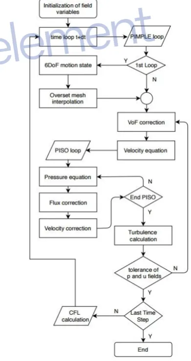
The solution algorithms which are under investigation for the time domain simulation of a ship after damage are PISO (Pressure Implicit with Splitting of Operator) and PIMPLE (Implicit Pressure Method for Pressure-Linked Equations). Both the algorithms are iterative solvers for transient simulations. PISO algorithm is suitable for CFL number below one. On the other hand, the PIMPLE algorithm is a combination of SIMPLE (Semi-Implicit Method for Pressure-Linked Equations) used for steady state problems and PISO (Moukalled, Mangani, & Darwish, 2016). PIMPLE algorithm is more flexible as it can be stable for CFL numbers bigger than one. Furthermore, it provides the opportunity for adjustment of the iterative procedure between convergence (speed) and stability (Holzmann, 2018; Foundation, 2014).

6. BENCHMARKING

A benchmark case is presented in the following section. The vessel in consideration is examined with time-domain simulation of flooding for a range of KG values. Following this, flooding simulation with CFD is performed.

The ship under investigation is a combat vessel with general particulars as presented in the following table. The damage condition under investigation is a four-compartment damage with the opening in the starboard side of the ship. The compartments R1, R2 are extended from port to starboard, and the two double bottom compartments from the centre line symmetry plane to starboard side. For demonstration purposes, the investigation is performed for four hypothetical KG values, 5.8 m, 6.71 m, 7.13 m , and 8.0 m respectively.

Table 1: Main Particulars of the vessel.

Main Particulars – Full scale

LBP 141.8 m Δmld 8684 t

Bmld 20.6 m LCG1 _{-0.65 m}

Tmld 7.49 m KGmld 7.84 m

Volumes of the Compartments

DB1 143.4 m3 _{R1 1,266.3 m}3

DB2 165.9 m3 _{R2 1,650.9 m}3

Figure 7: Profile view of the hull.

Figure 8: The four damaged compartments of the case under investigation.

1 _{The Longitudinal reference point is located}

amidships.

Figure 9: Midship section presenting the DB1, R1 compartments.

Static Stability

The first step in the stability assessment for the specific damage case is the calculation of the curve of static stability, GZ. For the calculation of the righting arm the method of lost buoyancy has been used.

Figure 10: Curves of static stability for the four KG values.

Time-Domain Simulations

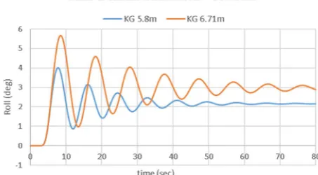
For the four cases under investigation time-domain simulation of flooding after damage has been performed. The tool, which has been used is PROTEUS3 and the results are presenting in the following graphs.

Figure 12: Roll response of the vessel for KG 7.13 m & 8.0 m.

The roll response follows the same pattern for all the cases. As the KG value increases the impact of flooding in the transient response of the vessel increases.

Verification with CFD

For CFD analysis, the OpenFOAM v1812 is used. The overInterDyMFoam solver is used for two incompressible, isothermal fluids with VOF interface capturing approach, incorporating optional overset mesh motion (Foundation, 2014). The forces and the moments on the hull are calculated with the coupling of sixDoFRigidBodyMotion library, which is provided with the package.

The CFD simulations have been performed in the Archie – WeSt High Performance Computing Facilities located at the University of Strathclyde. For each simulation 20 cores of Intel Xeon Gold 6138 have been used with frequency 2.0 GHz and 4.8 GB RAM per core.

Pre-Processing

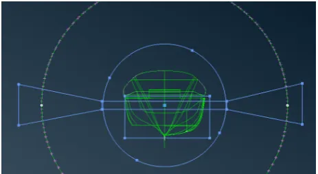
The pre-processing steps involve the preparation of the geometrical model and the generation of the grids, which will be used. The problem domain incorporates two main regions. The first is a cylinder with radius 2B, which includes the fluid domain in the vicinity of the hull and the four internal compartments of the ship. The second domain represents the earth-fixed environment in which the ship is moving and is used for the interpolation of the fluid variables from and to the overset region.

Figure 13: 3D representation of the hull.

Figure 14: The overset region which encompass the hall and the internal arrangement.

For grid generation, the ANSA v19.0.1 software has been used, developed by the BETA CAE. For the cylindrical volume of the overset region, the grid elements, which have been chosen are tetrahedral for two main reasons. The first is their ability to capture easier the geometry of the hull, and the edges inside the ship arrangement. Furthermore, unstructured tetrahedral elements provide the advantage of a smoother transition between the areas and volumes with different cell size. The smooth transition of the volumetric regions are crucial for the accurate velocity and pressure gradients and the stability of the solver.

Figure 16: The grid of the overset region.

The total number of cells of the overset region are presented in the following table.

Table 2: Mesh sizes.

Regions

Mesh Overset Background

Coarse 1,158,782 623,563

Medium 1,881,975 173,911

Fine 4,338,449 623,563

Figure 17: Fine mesh discretization close to the bulbous bow.

The background domain is a rectangular region developed only with hexahedral elements locally refined close to the free surface and the overset region where the interpolation of the fluid variables is performed.

Figure 18: The problem domain with the background and the overset mesh regions.

Simulation Set-Up

The set-up of the simulation has been chosen based on the demand of adequate accuracy and reasonable computational cost. For this reason the numerical tank uses the PIMPLE algorithm, which

allows large time steps without jeopardizing the stability of the calculation (Holzmann, 2018; Foundation, 2014). In the simulations, the time step control is based on the maximum CFL number in the domain and in the free-surface interface. Courant numbers have been chosen as

< 25 & free surface < 5 (22) For the control of PIMPLE the tolerance of the velocity and pressure fields have been set to the values of 10 and 10 , respectively. This is a conservative option as the aim was the stability of the simulation.

A very interesting and important topic in the CFD field is the selection of the appropriate turbulence model for the engineering problem under investigation. For this study, the kOmegaSST model has been chosen as it is the safest option for this kind of hydrodynamic problems (ITTC, 2011). For the capturing of the viscosity near the wall boundaries, the default wall faction which in provided for the CFD toolkit is implemented.

The results for the simulation of medium mesh in comparison with the results of the time-domain simulation for KG =7.13m are presented in the following figures.

Figure 4: A screenshot of the flooding at 4.0 sec.

The results obtained demonstrate the impact of floodwater dynamics in the roll response of the vessel. Initially, from 0.0 up to 4.0 seconds the ship rolls to the side of the damage with a maximum roll angle approximately 4 degrees, two degrees below the roll angle that the time domain simulation predicts. This phase is characterised by the motion of floodwater water front, resembling a dam-break phenomenon. From 4.5 sec, the roll angle starts to decrease and at 10 sec the vessel rolls to the port side with a maximum angle approximately -4.0 degrees. This stage is defined by the large hydrodynamic impact induced by the momentum of the floodwater to the port side of the hull. After the first 10 sec the synchronisation of the sloshing of the water inside the compartments and the motion of the hull produces a roll angle close to 10 degrees, the worst of the flooding scenario. After the initial transient stage the roll oscillation is decreased smoothly due to the damping of the motion of the hull. A very interesting outcome of the stationary stage is the smooth roll decade of the damaged hull.

In the figure, the roll response of the vessel as it has been calculated by CFD is presented. The agreement of the medium (2 m cells) and fine (4 m cells) mesh is notable. Furthermore, the coarse mesh calculates a maximum roll angle lower by approximately 3.5 degrees. The difference should be occurred due to the coarse background mesh and its impact in the interpolation of the flow variables with the overset region.

Figure 21: Mesh convergence analysis.

In terms of computational cost it has been noticed that the most important factor is the time step in each stage of the simulation. In the transient stage where the bigger CFL number is the waterfront of the floodwater the time step has a value close to 0.001. After the dam break phenomenon when the water touches the port side wall and up to the moment where the water reaches the maximum level

inside the compartment the maximum time step is approximately 0.005. In the steady stationary state, with maximum CFL limit 25, the time step increases to a value of 0.015. The optimized choice of time and space discretization is most vital factor for the reduction of the computational cost of the simulations.

7. CONCLUTIONS

This work presented the utilisation of CFD for the assessment of the survivability of a ship after damage. Despite the big computational cost related with high fidelity numerical simulations, it is proven that they can be an important tool in naval architect’s arsenal for the investigation of flooding of ship after damage. Time-domain simulation based on CFD can capture important phenomena that fast time-domain tools, based on hydraulic assumptions cannot, in a level of detail that sometimes is important. The discrepancies that have been between DTNS and CFD are under investigation. Furthermore, the selection of the time and space discretization is a key factor and it needs more research.

8. ACKNOWLEDGMENTS

The authors of this paper would like to express their gratitude to the sponsors of the Maritime Safety Research Centre, Royal Caribbean International & DNV – GL for their courtesy to support the research endeavours of the centre. Results were obtained using the ARCHIE-WeSt High Performance Computer (www.archie-west.ac.uk) based at the University of Strathclyde. Spacial thanks to the BETA CAE Systems (www.beta-cae.com) which supported this research work with for the provision of the advance pre - processing platform ANSA v19.0.1.

REFERENCES

Aguerre, H. J., Damian, S. M., Gimenez, J. M., & Nigro, N. M. (2013). Modelling of Compressible Fluid Problems with OpenFOAM Using Dynamic Mesh Technology. Associación Argentina de Mecánica Computacional.

Cummins, W. E. (1962). The Impulse Response Function and Ship Motions. Hydromechanics Laboratory Research and Development Report MIT.

Damian, S. M. (n.d.). Description and Utilization of interFoam Multiphase Solver. Final Work - Computatioanl Fluid Dynamics.

Ringwood, J. V. (2015). Implementation of an OpenFOAM Numerical Wave Tank for Energy Experiments. Proceedings of the 11th European Wave and Tidal Energy Conference. Nantes, France.

Ferziger, J. H., & Peric, M. (2002). Computational Methods for Fluid Dynamics (3rd ed.). Germany: Springer.

Foundation, O. (2014). OpenFOAM The OpenSource CFD Toolbox User Gide Version 2.3.0.

Gao, Z., Vassalos, D., & Gao, Q. (2010). Modelling water flooding into a damaged vessel by the VOF method. Journal of Ocean Engineering, 1428-1442.

Holzmann, T. (2018). Mathematics, Numerics, Derivations and

OpenFOAM(R). Holzmann CFD.

doi:10.13140/RG.2.2.27193.36960

ITTC. (2011). ITTC - Recommended Procedures and Guidelines. Practical Guidelines for Ship CFD Applications. International Towing Tank Conference.

Jasak, H. (1996). Error Analysis and Estimation in the Finite Volume Method with Applications to Fluid Flows. University of London: Ph.D thesis Imperial College.

Jasak, H. (2017). CFD Analysis in Subsea and Marine Technology. First Conference of Computational Methods in Offshore Technology. IOP Publishing.

Jasionowski, A. (2001). An Integrated Approach to Damage Ship Survivability Assessment. PhD thesis University of Strathclyde , Glasgow.

Jasionowski, A., Vassalos, D., & Guarian, L. (2004). Theoretical Developments on Survival Time Post - Damage. Proceedings of hte 7th Int Ship Stability Workshop. Shanghai.

Journee, J. M., Vermee, H., & Vredeveldt, A. W. (1997). Systematic Model Experiments on Flooding of Two RoRo Vessels. 6th International Conference on stability of Ships and Ocean Vehicles, (pp. 81-98). Varna, Bulgaria.

Letizia, L., & Vassalos, D. (1995). Formulatiion of a Non -Linear Mathematical Model for a Damaged Ship with Progressive Flooding. International Symposium on Ship safery in a Seaway, (p. 20pp). Kaliningrand, Russia.

MARIN. (2003). Large Passenger Ship Safety. Time-to-flood simulations for a large passenger ship - initial study. IMO, Sub-Committee on Stability and Load Line and on SIshing Vessels Safety, 46th session, Agenda item 8.

Moukalled, F., Mangani, L., & Darwish, M. (2016). The Finite Volume Method in Computational Fluid Dynamics. An Advanced Introduction with OpenFOAM(R) and Matlab(R). Springer International Publishing Switzerland.

Papanikolaou, A. D. (2007). Review of damage stability of ships

recent developments and trends. Proceedings 10th Int. Symposium on Practical Design of Ships and Other Floating Structures. Houston.

Papanikolaou, A., & Spanos, D. (2002). On the Modelling of Floodwater Dynamics and its Effects on Ship Motion. 6th International Ship Stability Workshop. New York: Webb Institute.

Peric, M. (2018). Best practices for wave flow simulations. The Naval Architect International Journal of the Royal Institute of Naval Architects (RINA).

Roenby, J., Larsen, B. E., Bredmose, H., & Jasak, H. (2017). A new volume-of-fluid method in OpenFOAM. VII International Conference on Computational Methods in Marine Egineering MARINE.

Ruponen, P. (2007). Progressive Flooding of a Damaged Passenger Ship Docoral Dissertation. Esploo, FInland: Helsinki University of Technology.

Sadat-Hosseini, H., Kim, D. H., Lee, S. K., Rhee, S. H., Carrica, P., Stern, F., & Rhee, K.-P. (2012). CFD and EFD Study of Damaged Ship Stability in Calm Water and Regular Waves. Proceeding of the 11th International Conference on the Stability of Ships and Ocean Vehicles, (pp. 425-452). Athens, Greece.

Santos, A., & Soares, G. (2006). Study of the Dyanamics of a Damaged RoRo Passenger Ship. 9th International Conference on Stability of Ships and Ocean Vehicles. Rio de Janeiro, Brazil.

Shen, L., & Vassalos, D. (2011). Application of 3D Parallel SPH to Ship Sloshing and Flooding. In Contemporary Ideas on Ship Stability and Capsizing in Waves (pp. 709-721). Springer.

Skaar, D., & Vassalos, D. (2006). The Use of a Mesh-less CFD Method to Model the Progressive Flooding of a Damaged Ship. 9th International Conference on the Stability of Ships and Ocean Vehicles. Rio de Janeiro, Brazil.

So, K. K., Hu, X. Y., & Adams, N. A. (2009). Anti - diffusion method for interface steeping in two - phase incompressible flow.

Spanos, D., & Papanikolaou, A. (2001). Numerical Study of the Damage Stability of Ships in Intermediate Stages of Flooding. 5th International Workshop of Stability and Operational Safety od Ships. Trieste: University of Trieste.

Spouge, J. R. (1985). The technical investigation of the sinking of the Ro Ro Ferry European Getaway. Transactions of RINA, 49-72.

Proc. 10th International Conference of Stability of Ships & Ocean Vehicles, (pp. 733-740). St. Petersburg, Russia.

van't Veer, R., & de Kat, O. (2000). Experimental adn Numerical Investigation on Progressive Flooding in Complex Compartment Geometries. Proceedings of the 7th International Conference on Stability of Ships and Ocean Vehicles, (pp. 305-321). Lainceston, Tasmania, Australia.

Vassalos, D. (2000). The Water on Deck Problem of Damaged Ro-Ro Ferries. Contemporary Ideas on Ship Stability , Elsevier, 163-185.

Vassalos, D. (2009). Risk - Based Ship Design Methods, Tools and Applications. (A. Papanikolaou, Ed.) Veerlag Berlin Heidelberg: Springer.

Vassalos, D. (2014). Damage Stability and Survivability -'nailing' passenger ship safety problems. Ship and Offshore Structures, 9(3), 237-256.

Vassalos, D., & Turan, O. (1994). A Realistic Approach to Assessing the Damage Survivability of Passenger Ships. Transactions of Society of Naval Architects and Marine Engineers,SNAME, Vol 102, 367-394.

Vassalos, D., Atzampos, G., Cichowicz, J., Karolius, K. B.,

Boulougouris, E., Svensen, T., . . . Luhmann, H. (2018). Life-Cycle flooding risk management of passenger ships. 13th International Conference of Stability of Ships and Ocean Vehicles , (pp. 648-662). Kobe, Japan.

Vassalos, D., Jasionowski, A., & Guarin, L. (2006). Passenger Ships Safety - Science Paving the Way. Journal of Marine Science and Technology, 63-71.

Vassalos, D., Turan, O., & Pawlowski, M. (1997). Dynamic stability assessment of damaged passenger/Ro-Ro ships and proposal of rational survival critiria. Marine Technology, 34(4), 241-266.

Vredeveldt, A. W., & Journee, J. M. (1991). Roll motions of ships due to sudden water ingress, calculations and experiments. RINA International Conference on Ro Ro Safety and Vulnerability the Way Ahead. London, UK: RINA.