City, University of London Institutional Repository
Citation
: Rendon-Sanchez, J. (2016). Structure combination of forecasting models with
application in the energy sector. (Unpublished Doctoral thesis, City, University of London)This is the accepted version of the paper.
This version of the publication may differ from the final published
version.
Permanent repository link:
http://openaccess.city.ac.uk/17942/Link to published version
:
Copyright and reuse:
City Research Online aims to make research
outputs of City, University of London available to a wider audience.
Copyright and Moral Rights remain with the author(s) and/or copyright
holders. URLs from City Research Online may be freely distributed and
linked to.
City Research Online: http://openaccess.city.ac.uk/ [email protected]
Structure Combination of Forecasting
Models
with Applications in the Energy Sector
By
Juan F. Rendon-Sanchez
Supervisors
Professor Lilian M. de Menezes
Professor ManMohan Sodhi
A dissertation submitted to City, University of London, in accordance with the requirements of the degree of
Doctor of Philosophy in Management.
City
University of London
Faculty of Management
Cass Business School
Contents
List of Tables . . . 9
List of Figures . . . 13
Acknowledgements . . . 17
Declaration of Authorship . . . 18
Abstract . . . 19
Nomenclature . . . 21
1 Introduction 25 2 Literature Review 31 2.1 Combination of Forecasts . . . 31
2.1.1 The Motivation for Combining Forecasts . . . 31
2.1.2 The Most Common Methods for Combining Forecasts . . . 32
2.1.2.1 Statistical Based Approaches . . . 32
2.1.2.2 Computational Intelligence Approaches . . . 35
2.1.2.3 Ensembles of NN . . . 36
2.2 Examples of Applications of Combinations in the Energy Sector . . . 40
2.2.1 Applications in Load Forecasting . . . 41
2.2.2 Applications in Wind Power Forecasting . . . 46
2.2.3 Other Applications . . . 49
2.3 The Current State of the Literature on Ensembles for Time Series Forecasting . . . 51
2.4 Research Questions . . . 61
3 A Sensitivity Analysis of the Performance of Feed-Forward Neural
Networks 65
3.1 Abstract . . . 65
3.2 Introduction . . . 66
3.3 The Synthetic Time Series . . . 70
3.4 Design . . . 77
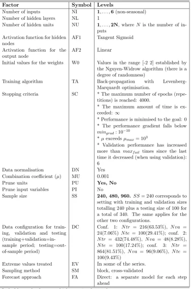
3.4.1 Choice of Factors, Levels, and Ranges . . . 77
3.4.2 Selection of the Response Variable . . . 81
3.4.3 Choice of Experimental Design . . . 82
3.4.4 Methodology to Perform the Experiments . . . 82
3.4.5 Statistical Analysis of Design Factors . . . 83
3.5 Results . . . 85
3.6 Discussion . . . 96
3.7 Conclusions and Further Research . . . 101
4 Structural Combination of Neural Network Forecasting Models 105 4.1 Abstract . . . 105
4.2 Introduction . . . 106
4.3 Methodology . . . 108
4.3.1 Randomisation of Input-Output Patterns . . . 109
4.3.2 Structural Combination Based on Clustering (CB) . . . 110
4.3.2.1 The Forecasting Model . . . 113
4.3.2.2 Assessment of Uncertainty in the Forecast . . . 116
4.3.3 Structural Combination Based on Genetic Algorithms (GA) . 117 4.4 The Empirical Studies . . . 119
4.4.1 Analysis Procedure . . . 123
4.5 Studies with Synthetic Series . . . 125
4.5.2 Synthetic-1S Series . . . 135
4.5.3 Synthetic-2S Series . . . 146
4.6 Discussion of Findings from Synthetic Series . . . 158
4.7 Forecasting Wind Power Using Ensembles of NNs Based on Multi-variate Time Series . . . 161
4.7.1 Preliminary Analysis and Specification of Individual Models . 163 4.7.2 Combination of Models . . . 169
4.8 Study with an Electricity Demand Time Series . . . 183
4.8.1 Variant of the Model for an Iterative Forecast . . . 184
4.8.2 Preliminary Analysis and Specification of Individual Models . 185 4.8.3 Combination of Models . . . 192
4.9 Discussion of Findings from Real Time Series . . . 203
4.10 Discussion of Findings in the Context of Ensembles . . . 204
4.11 Conclusions and Research Agenda . . . 208
5 Structural Combination of Seasonal Exponential Smoothing Mod-els 213 5.1 Abstract . . . 213
5.2 Introduction . . . 214
5.3 The Base Models . . . 216
5.4 Methodology . . . 217
5.4.1 Block Swapping and Noise Addition . . . 218
5.4.2 Experimental Setup . . . 222
5.4.3 Analysis Procedure . . . 222
5.5 Structural Combinations of MHW Models to Forecast Daily Peak Electricity Demand . . . 224
5.5.2 Results when Model Variation was Introduced through Block
Swapping to Generate MHW Combinations . . . 230
5.6 Structural Combinations of MHWT Models to Forecast Rio de Janeiro
Electricity Demand . . . 236
5.6.1 Results when Model Variation was Introduced through Noise
Addition to Generate MHWT Combinations . . . 237
5.6.2 Results when Model Variation was Introduced through Block
Swapping to Generate MHWT Combinations . . . 241
5.7 Structural Combinations of MHWT Models to Forecast England and
Wales Electricity Demand . . . 248
5.7.1 Results when Model Variation was Introduced through Noise
Addition to Generate MHWT Combinations . . . 249
5.7.2 Results when Model Variation was Introduced through Block
Swapping to Generate MHWT Combinations . . . 254
5.8 Discussion . . . 260
5.9 Conclusions and Research Agenda . . . 265
6 Summary and Directions for Future Research 269
6.1 A Sensitivity Analysis of the Performance of Feed-Forward Neural
Networks . . . 270
6.2 Structural Combination of Neural Network Forecasting Models . . . . 273
6.3 Structural Combination of Seasonal Exponential Smoothing Models . 276
6.4 Implications for the Literature and Future Research . . . 278
6.5 Main Contributions of this Research . . . 285
Bibliography 287
B Selected Model Configurations for Sample Series 311
C Additional Material for the Chapter on Structural Combination of
Neural Networks 313
C.1 STAR2 Time Series . . . 313
C.2 Synthetic-1S Time Series . . . 316
C.3 Synthetic-2S Series . . . 318
C.4 Wind Power Time Series . . . 320
List of Tables
2.1 Ensemble generation schemes. . . 55
3.1 Factors used in the sensitivity analysis for neural networks. . . 80
3.2 Summary of findings for the sensitivity analysis. . . 91
3.3 Direction of the contribution of a factor . . . 97
3.4 Summary of factor influence . . . 98
4.1 Configuration of the clustering combination algorithm. . . 121
4.2 Configuration of individual networks. . . 121
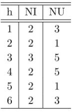
4.3 Selected NN models for STAR2 series. . . 126
4.4 Forecasting performance. STAR2 series. . . 130
4.5 Coefficients for structural combination. STAR2 series (M axC = 4) . 132 4.6 Ljung-Box test. Series: STAR2 . . . 132
4.7 Cluster validity indexes. Series: STAR2. . . 134
4.8 Selected NN models for Synthetic-1S series. . . 136
4.9 Forecasting performance. Synthetic-1S series . . . 140
4.10 Coefficients for structural combination. Synthetic-1S series (M axC= 8). . . 143
4.11 Cluster validity indexes. Series: Synthetic-1S. . . 145
4.12 Selected NN models for Synthetic-2S series. . . 147
4.13 Forecasting performance. Synthetic-2S series . . . 152
4.14 Coefficients for structural combination. Synthetic-2S series (M axC= 8) . . . 156
4.15 Cluster validity indexes. Series: Synthetic-2S. . . 157
4.17 Configuration of the sensitivity analysis for neural networks (Kaggle
wind power data) . . . 164
4.18 Models with the lowest average out-of-sample RMSE. . . 165
4.19 Selected models for Kaggle series. . . 169
4.20 Forecasting performance. Series: Kaggle wind power . . . 173
4.21 Coefficients for structural combination. Series: Kaggle wind power (M axC= 8) . . . 179
4.22 Cluster validity indexes. Series: Kaggle wind power production. . . 180
4.23 Comparisons by forecast horizon. Series: Kaggle wind power . . . 182
4.24 Ljung-Box test. Series: Kaggle wind power . . . 183
4.25 Factor configuration. Sensitivity analysis for neural networks. Series: Rio de Janeiro electricity demand . . . 186
4.26 Model with the lowest average out-of-sample MAPE. . . 187
4.27 Forecasting performance. Series: Rio de Janeiro electricity demand . 198 4.28 Jarque-Bera normality test. Series: Rio de Janeiro electricity demand 201 4.29 Coefficients for structural combination of NN. Series: Rio de Janeiro electricity demand. . . 201
4.30 Comparisons by forecast horizon. Series: Rio de Janeiro electricity demand. . . 202
4.31 Cluster validity indexes. Series: Rio de Janeiro electricity demand. . . 202
5.1 Sample MHW models with noise addition. Series: Rio de Janeiro peak electricity demand. . . 229
5.2 Coefficients for sample CB combination of MHW models with noise addition. Series: Rio de Janeiro peak electricity demand. . . 229
5.4 Coefficients for sample CB combination of MHW models with block
swapping. Series: Rio de Janeiro peak electricity demand . . . 233
5.5 Sample MHWT models with noise addition. Series: Rio de Janeiro
electricity demand. . . 240
5.6 Coefficients for sample CB combination of MHWT models with noise
addition. Series: Rio de Janeiro electricity demand . . . 240
5.7 Jarque-Bera test of forecast errors for HWT combinations (low noise,
Rio de Janeiro electricity demand) . . . 241
5.8 Jarque-Bera test of forecast errors for HWT combinations (medium
noise, Rio de Janeiro electricity demand) . . . 241
5.9 Sample MHWT models with block swapping. Series: Rio de Janeiro
electricity demand. . . 245
5.10 Coefficients for sample CB combination with block swapping. Series:
Rio de Janeiro electricity demand . . . 245
5.11 Sample MHWT models with noise addition. Series: England and
Wales electricity demand. . . 253
5.12 Coefficients for sample CB combination of MHWT models with noise
addition. Series: England and Wales electricity demand . . . 253
5.13 Sample double seasonal models with block swapping. Series: England
and Wales electricity demand. . . 257
5.14 Coefficients for sample CB combination of MHWT models with block
swapping. Series: England and Wales demand . . . 257
5.15 Summary of findings for structural combinations. . . 266
List of Figures
2.1 General steps in ensemble generation. . . 51
3.1 General steps in ensemble generation with DOE. . . 67
3.2 Illustration of single-seasonal synthetic time series generation. . . 72
3.3 Simulated series (non-seasonal). . . 74
3.4 Simulated series (seasonal). . . 76
3.5 Rolling window for training (fitting with in-sample data) and testing with out-of-sample data. . . 81
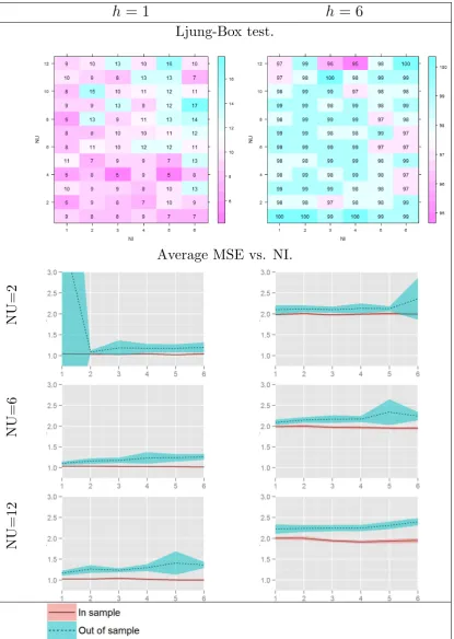
3.6 SAR series summary. . . 86
3.7 SAR series summary. . . 87
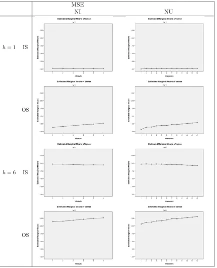
3.8 Main effects. Series: SAR. . . 90
3.9 Summary of Average MSE vs. NI (number of lagged inputs). . . 94
4.1 Multi-layer perceptron. . . 107
4.2 Modelling process. . . 109
4.3 Structural combination based on clustering. . . 115
4.4 Structural combination based on genetic algorithms. . . 118
4.5 STAR2 series. . . 125
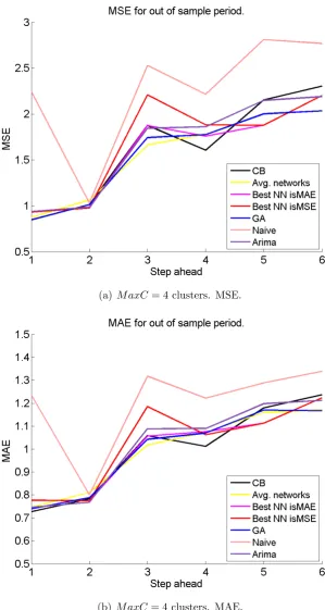
4.6 Out-of-sample MSE and MAE for STAR2 series. . . 127
4.7 Out-of-sample MSE for STAR2 series. . . 128
4.8 Out-of-sample MSE vs. number of clusters. STAR2 series. . . 128
4.9 Forecast intervals for STAR2 time series . . . 133
4.10 Synthetic-1S series. . . 135
4.11 Out-of-sample MSE and MAPE for Synthetic-1S series. . . 137
4.13 Out-of-sample MSE vs. number of clusters. Synthetic-1S series. . . . 139
4.14 Forecast intervals for Synthetic-1S time series . . . 144
4.15 Synthetic-2S series . . . 146
4.16 Out-of-sample MSE and MAPE for Synthetic-2S series . . . 148
4.17 Out-of-sample MSE for Synthetic-2S series. . . 149
4.18 Out-of-sample MSE vs. number of clusters. Synthetic-2S series. . . . 150
4.19 Forecast intervals for Synthetic-2S time series . . . 155
4.20 Hourly electricity production for Kaggle wind farm 1 . . . 163
4.21 Average NMAPE% and RMSE vs. forecast horizon. Series: Kaggle wind power . . . 165
4.22 Weather forecasts usage. . . 165
4.23 Main effects. Series: Kaggle wind power . . . 167
4.24 Out-of-sample NMAPE and RMSE. Series: Kaggle wind power . . . . 171
4.25 Out-of-sample RMSE. Series: Kaggle wind power . . . 172
4.26 Out-of-sample RMSE vs. number of clusters. Series: Kaggle wind power . . . 177
4.27 Forecast intervals. Series: Kaggle wind power . . . 178
4.28 Hourly electricity demand in Rio de Janeiro. . . 184
4.29 Replications of Rio de Janeiro electricity demand time series . . . 188
4.30 Average MAPE vs. forecast horizon. Series: Rio de Janeiro electricity demand . . . 189
4.31 Main effects. Series: Rio de Janeiro electricity demand . . . 190
4.32 Out-of-sample MAPE and MSE. Series: Rio de Janeiro electricity demand. . . 194
4.35 Forecast intervals. Series:Rio de Janeiro electricity demand. . . 197
5.1 Model scheme. . . 218
5.2 Block swapping . . . 221
5.3 Daily peak electricity demand in Rio de Janeiro . . . 224
5.4 Summary for Rio de Janeiro peak electricity demand under noise addition. 226 5.5 %∆ MAPE comparisons for Rio peak demand (noise addition). . . . 227
5.6 Summary for Rio de Janeiro peak electricity demand under block swapping.231 5.7 %∆ MAPE comparisons for Rio peak demand (block swapping). . . . 232
5.8 Best ensemble-based models for Rio de Janeiro peak electricity demand. . 235
5.9 Hourly electricity demand in Rio de Janeiro . . . 236
5.10 Summary for Rio de Janeiro hourly demand under noise addition.. . . 238
5.11 %∆ MAPE comparisons for Rio hourly demand (noise addition). . . . 239
5.12 Summary for Rio de Janeiro hourly demand under block swapping. . . 243
5.13 %∆ MAPE comparisons for Rio hourly demand (block swapping). . . 244
5.14 Best ensemble-based models for Rio de Janeiro electricity demand. . . 246
5.15 Rank of best ensemble-based models for Rio de Janeiro demand series. . . 247
5.16 Half-hourly electricity demand in England and Wales . . . 249
5.17 Summary for England and Wales half-hourly demand under noise addition.251 5.18 %∆ MAPE comparisons for England and Wales series (noise addition).252 5.19 Summary for England and Wales half-hourly demand under block swapping.255 5.20 %∆ MAPE comparisons for England and Wales (block swapping). . . 256
5.21 Best ensemble-based models for England and Wales demand series. . . 258
5.22 Rank of best ensemble-based models for England and Wales demand series.259 C.1 Out-of-sample MSE and MAE for STAR2 series. . . 314
C.2 Out-of-sample MSE for STAR2 series. . . 315
C.4 Out-of-sample MSE for Synthetic-1S series. . . 317
C.5 Out-of-sample MSE and MAPE for Synthetic-2S series . . . 318
C.6 Out-of-sample MSE for Synthetic-2S series. . . 319
C.7 Out-of-sample NMAPE and RMSE. Series: Kaggle wind power . . . . 320
C.8 Out-of-sample RMSE. Series: Kaggle wind power . . . 321
C.9 Out-of-sample MAPE and MSE. Series: Rio de Janeiro electricity
demand. . . 322
Acknowledgements
I am deeply indebted to my supervisor, Professor Lilian De Menezes, who
con-stantly and generously provided me with technical and intellectual guidance and
support.
I owe sincere thankfulness to Professor James Taylor and Dr. Siddharth Arora for
generously providing their Matlab code for the double-seasonal Holt-Winters-Taylor
model and data from some of their studies. I am indebted to Dr. Eduardo Alonso,
Dr. Sven Crone and Dr. Nikolay Nikolaev who helped me with their constructive
comments and kindly provided valuable information and advise.
I sincerely thank City University and Cass Business School for their generosity.
Specially I thank Malla Pratt for her constant support.
I profoundly thank my mother, Olga Sanchez, for her constant encouragement
and support. I am also grateful to all members of my extended family who helped
me at different points of this research, specially my aunt, Fanny Sanchez, and my
cousins Carolina Perez and Cesar Perez.
I thank Priscila Dahiana Gato for her love, company and encouragement.
My friends, Melanie Said, Andres Villegas, Maryam Lofti, Kaizad Doctor,
Mar-ianna Russo, Christopher Benoit, Danilo Mandic, Elena Casprini, Madona Zoraida,
Juan Carlos Aristizabal and Laura Mena, were a source of strength and help. I am
fortunate of having found them along my way.
I am also indebted to the Free Software Foundation, the Debian, Linux Mint,
Ubuntu, PostgreSQL, GIMP, GNU Emacs and LATEX projects for their amazing
Declaration Of Authorship
I, Juan F. Rendon-Sanchez, declare that this thesis titled, “Structure
Combina-tion of Forecasting Models with ApplicaCombina-tions in the Energy Sector” and the work
presented in it are my own. I confirm that:
This work was done wholly or mainly while in candidature for a research degree
at this University.
Where any part of this thesis has previously been submitted for a degree or
any other qualification at this University or any other institution, this has
been clearly stated.
Where I have consulted the published work of others, this is always clearly
attributed.
Where I have quoted from the work of others, the source is always given. With
the exception of such quotations, this thesis is entirely my own work.
I have acknowledged all main sources of help.
Where the thesis is based on work done by myself jointly with others, I have
made clear exactly what was done by others and what I have contributed
my-self.
Signed:
Abstract
This dissertation proposes and implements the inclusion of model structure in combining forecasts. Empirical investigations are conducted with an emphasis on neural networks and seasonal exponential smoothing models using synthetic data and real time series, from the electricity sector. It starts with a literature review on combining forecasts and ensembles of neural networks, and highlights their use in forecasting within the energy sector. Research gaps are identified and the questions to be addressed in this research are set, thus leading to three empirical studies.
The first study provides a detailed sensitivity analysis of the goodness-of-fit and forecasting performance of feed-forward neural networks on time series with different characteristics. It expands existing literature by increasing the number and variety of time series and by using graphical and statistical diagnostics to objectively judge the influence of model specification on forecasting performance. Having identified conditions for achieving stable model performance, this study facilitated the iden-tification of suitable models for different time series characteristics, which are then useful in developing combinations (ensembles) of feed-forward neural networks.
The second study proposes structural combination methods based on clustering (CB) and genetic algorithms (GA) for forecasting time series. Clustering of neural networks using their parameter space is performed to identify a pool of forecasts to be combined. Three synthetic time series and two real time series (electricity demand and wind power production) were used to assess the performance of the two proposals against several benchmarks in univariate and multivariate forecasting
problems. Structural combinations with GA were more competitive than those
with CB for non-seasonal time series and the multivariate wind power forecasting application, whereas for the seasonal series, the CB tended to be more competitive. The third study focused on forecasting univariate time series with seasonality, by structurally combining, in separate applications, multiplicative Holt-Winters and multiplicative Holt-Winters-Taylor models. Noise addition and block swapping were applied to the original time series in order to generate structurally diverse individual models. Applications were conducted using a seasonal daily peak electricity demand time series, an hourly double-seasonal electricity demand series and a half-hourly double-seasonal electricity demand series. Structural combinations worked better for the peak electricity demand and half-hourly demand time series when model variation was induced via noise addition. For the double-seasonal hourly electricity demand, block swapping, as a means for diversity in models, resulted in better forecasts.
Nomenclature
%∆ wrt Avg.: Percentage difference of an error metric with respect to the forecast
average from all models in the ensemble.
AFTER: Aggregated Forecast Through Exponential Re-weighting.
AHWT: Double-seasonal Holt-Winters-Taylor model in its additive form.
ARMAX: ARIMA models with exogenous variables.
Avg. Net.: forecast average from all neural network models in an ensemble.
Best Net. isMAPE: Neural network with the lowest in-sample MAPE in an
ensem-ble.
Best Net. isMSE: Neural network with the lowest in-sample MSE in an ensemble.
DGP: Data Generating Process.
DOE: Design of Experiments.
GA: Genetic Algorithms.
IS MAE: MAE for the in-sample period.
IS MSE: MSE for the in-sample period.
IS NMAPE: NMAPE for the in-sample period.
IS RMSE: RMSE for the in-sample period.
J-T: Jonckheere-Terpstra test.
LB TEST: Ljung-Box test for serial correlation.
MAE: Mean Absolute Error.
MAP: Maximum Absolute Percentage Error.
MAPE: Mean Absolute Percentage Error.
MHW: Single-seasonal Holt-Winters model in its multiplicative form.
MHWT: Double-seasonal Holt-Winters-Taylor model in its multiplicative form.
MIMO: Multiple-Input Multiple-Output approach for multi-step ahead forecasts
with NN.
MISMO: Multiple-Input Several Multiple-Outputs approach for multi-step ahead
forecasts with NN.
MM5: Fifth generation Mesoscale Model.
MSE: Mean Square Error.
MSPE Mean squared prediction error.
MVE: Mean-variance estimation. Method to estimate neural network-based
predic-tion intervals.
NMAPE: Normalised Mean Absolute Percentage Error.
NN: Neural Network.
OS MAE: MAE for the out-of-sample period.
OS MSE: MSE for the out-of-sample period.
OS RMSE: RMSE for the out-of-sample period.
RBF: Radial Basis Function.
RMSE: Root Mean Square Error.
SMAPE: Symmetric mean absolute percentage error.
SOM: Self Organising Maps.
THEIL: Theil Inequality Coefficient.
Chapter 1
Introduction
There has been over forty years of research in forecast combinations. The interest
from academics and practitioners signals the recognition of limitations of
individ-ual forecasting models and the desire to exploit the advantages of multiple models.
Nowadays, people and organisations are confronted with complex problems,
consid-erable uncertainties as well as an abundance of data and forecasting approaches.
Efforts are easily discernible toward the exploitation of a wide choice of data, of
forecasting models and scenarios in order to seek better forecasting performance
and, if possible, to quantify the uncertainty in the forecasts (Taylor & Buizza, 2003;
Stephenson et al., 2005; Taylor et al., 2009; Lemke & Gabrys, 2010). However, most
of the research has focused on how to combine forecasts produced by models and
experts. Little attention has been given to the combination of models based on their
specification.
Variety in structure stems from differences in the functional form of models
or differences in their parameter values. Consider a model ARIM A(p, d, q) with
parameters Θ and Φ. This model would have structural differences (in terms of
functional form) when compared to a model ARIM A(p0, d0, q0) if p 6= p0, d 6= d0
or q 6= q0. On the other hand, when several ARIM A(p, d, r) models are produced
with different Θ and Φ coefficients, variety in structure results from differences in
parameters and not from their functional form. Analogously, a feed-forward neural
network, fitted to a time series, can have different specifications, depending on the
number of hidden units, the number of hidden layers, the transfer function, the
units sets {w} and {w0} would differ, all other factors constant, when the number of hidden units in {w} and {w0} differ or the values are different, and thus they be structurally different. The main goal of this research is to use this structural
information when combining forecasts.
In structural combinations, the generation of different forecasting models,
pre-vious to the calculation of the combination, arises naturally. The systematic
gen-eration and combination of forecasting models has been traditionally considered in
the Neural Network literature under the term ensembles. This term originated in
climate modelling, when it was observed that there are differences in forecasts when
models are initialised with different values (Parker, 2010). The building of
ensem-bles has evolved from the use of simple sets of models to the collective evolution
of them through sophisticated computational intelligence techniques. An ensemble
generally has three stages (Leith, 1974; Lorenz, 1965; Hansen & Salamon, 1990):
the generation of models, their selection or pruning and their combination. It is
within this framework that the present research is located and attempts to make a
contribution. In doing so, this dissertation aims at bringing models that have been
found to be robust in the forecasting literature to the context of ensemble building
and machine learning.
The first models considered are feed-forward neural networks, because of their
natural structural representation, which is related to their founding idea of imitating
the brain structure (see Haykin, 1999, p.24), and their use in ensembles.
Further-more, neural networks are widely applied in forecasting problems. IEEE archives
(with publications in Operations and Management starting from 1990 to 2015) reveal
that they have been widely applied, with publications in transport (10), education
(11), mail (5), telephone systems (14), gas (186), water (207) and specially in power
systems (886)1. The predominance of applications in the energy sector motivates
the current research. Secondly, two statistical models are considered: the
single-seasonal multiplicative Holt-Winters model and the double-single-seasonal multiplicative
Holt-Winters-Taylor model. The former belongs to a family of models used to
fore-cast seasonal time series due to their robustness and simplicity (Hyndman et al.,
2008; Pan, 2010), and the latter is an extension that has been applied successfully
to electricity load forecasting (Taylor et al., 2006; Taylor, 2010).
Given the choice of models available in the literature, the general enquiry of this
dissertation is cast into the following research questions: How can the structure of
neural network forecasting models be combined? How can the structural combination
be extended from neural networks to other forecasting models?
These questions focus on the last stage of building ensembles, that is, the
ag-gregation of forecasts after the models were generated. However, the initial stage
(the specification of models) also requires attention, since one would like to combine
models that are robust. The study of the behaviour of models to be included in
the ensemble facilitates making decisions when building ensembles. The need for
such a study is acutely felt when using neural networks, given that they are
uni-versal approximators with a structure that can be modified depending on specific
needs and desired precision (Haykin, 1999). Additionally, the use of statistical tools
has been essential in understanding the behaviour of neural networks in order to
make a better use of them (Anders & Korn, 1999). The design of experiments is
here adopted, as it allows to systematically examine the effect of different design
factors in goodness-of-fit and accuracy of NNs. Although there have been studies
of NNs in this direction, as for example Zhang et al. (2001) and Balestrassi et al.
(2009), they were limited to one-step-ahead forecasting and have not considered the
double seasonal series that are common in short-term forecasting of electricity
de-mand. Therefore, an initial study is conducted, which focuses on sensitivity analysis,
models to build ensembles.
The exploration of structural combination can inform the literature on forecast
combination, which in turn can open avenues to improve forecasting accuracy by
making use of more diverse sources of information than normally considered when
combining forecasts. Although most of the applications made here use data from
the energy sector, it would be expected that other complex forecasting problems
could benefit from structural combinations of models, specially in the context of big
data and business analytics.
This dissertation investigates combinations or ensembles of forecasts, neural
net-work sensitivity and structural model combination, in the following way:
Chapter 2 reviews relevant literature in the area of neural network ensembles
and forecast combination, with an emphasis on applications in the energy sector
and concludes with setting the research questions to be addressed by this research.
In Chapter 3, sensitivity analyses of neural networks are conducted, using synthetic
time series, and guidelines are suggested to aid model selection. In Chapter 4, a
structural combination approach for neural network is proposed and applications are
conducted with synthetic and real world time series (electricity demand data from
Rio de Janeiro and wind power production data from the global Energy Forecasting
Competition, 2012). The investigation concentrates on ensembles with structural
parameter variation, while keeping the same functional form. The selection of models
to include in the structural combination is conducted along the lines suggested by the
analysis developed in Chapter 3. Chapter 5 explores the behaviour of the proposed
structural combination focusing on the single-seasonal multiplicative Holt-Winters
and the double-seasonal multiplicative Holt-Winters-Taylor models. Applications
are conducted with a daily peak electricity demand time series, and two electricity
demand time series (hourly observations from Rio de Janeiro and half-hourly
Chapter 2
Literature Review
This chapter reviews the literature on forecast combination with an emphasis on the
energy sector and neural networks (NN) ensembles. The choice of these models is
motivated by their suitability for structural model combination, which is the main
aim of this dissertation, and also by the extensive use of such models in forecasting
electricity demand as highlighted in previous reviews of this literature (Hippert
et al., 2001; Crone et al., 2011). At the end of the chapter gaps in the literature are
highlighted and research questions are formulated.
2.1
Combination of Forecasts
2.1.1
The Motivation for Combining Forecasts
There are several reasons for combining forecasts (Clemen, 1989; Timmermann,
2006). If it is assumed that the information set underlying the individual forecasts is
often unobserved to the forecast user, then it is not possible to gather all information
and construct a “super” model. In this case, the combination of forecasts will be an
attempt to optimise the use of information that is available to the forecaster.
Some models may adapt quicker than others to changes in the data generating
process. As it is difficult to detect structural breaks in “real time” it is plausible
that, on average, combinations of forecasts from models with different degrees of
adaptability will outperform forecasts from individual models. Furthermore,
indi-vidual forecast models may be subject to misspecification bias of unknown form.
more robust.
In general, there is a growing consensus about the advantages of combining
fore-casts. Clemen (1989), while reviewing empirical evidence in forecast combination,
concluded that combining multiple forecasts leads to increased forecast accuracy.
Stock & Watson (2004) observed, after an empirical analysis that included data
adaptivity weighting mechanisms, that forecast combination performs well with
respect to autoregressive models. They also concluded that the best performing
combination schemes were simple ones, such as the average and models with the
most simple data adaptivity in their weighting schemes. Timmermann (2006)
ar-gued, from a theoretical perspective, that unless one can find ex ante a particular
forecasting model producing smaller forecast errors than its competitors, forecast
combination offers diversification gains that make it attractive to combine
individ-ual models rather than relying on a forecast from a single model.
2.1.2
The Most Common Methods for Combining Forecasts
Statistical approaches (such as linear combinations and clustering) and
computa-tional intelligence models (such as fuzzy logic and NN) have been used to combine
forecasts.
2.1.2.1 Statistical Based Approaches
Linear combination is one of the simplest forecast combination methods. The simple
average is difficult to defeat (Armstrong, 2001). Che (2015) suggest improvements
to the selection of models for linear combinations. The concept of entropy1 and
co-variance between forecasts are used to define the amount of common linear
infor-mation between a set of forecasts and the actual value. The relevance of a random
independent variable (a forecast) with respect to the dependent variable (the actual
1Entropy is a measure of the uncertainty of a random variable (Cover & Thomas, 2006, p. 13). For a discrete random variableX, it is defined asH(X) =−P
value) is defined in a similar way. The redundancy (when the common linear
infor-mation is maximum) and the relevance are then used to select forecasting models
for a combination; the approach minimises linear redundancy and maximises linear
relevance. This procedure allows for an algorithm to find the optimal subset of all
the individual models to combine without having to try all possible combinations of
the individual models.
Outperformance (Bunn, 1975) is a form of combination that has the form fc =
p0f, where f is a vector of forecasts and fc is the resulting forecast. It uses p, a
simplex of probabilities which can be assessed and revised in a Bayesian manner. In
practice,pis the historical proportion that the forecaster or model has outperformed
its competitors. Each individual weight is interpreted as the probability that its
respective forecast will be the best (in the smallest absolute error sense) on the next
occasion.
In the optimal approach (Bates & Granger, 1969), linear weights are calculated
to minimise the error variance of the combination (assuming unbiasedness for each
individual forecast). The vector of combining weights, w, is determined according
to the formula w = eS0S−−11ee, where e is the (n×1) unit vector and S is the (n×n) covariance matrix of forecast errors. The authors also proposed variations to this
approach, namely, theoptimal (adaptive) with independence assumption in which the
estimate ofSis restricted to be diagonal, comprising just the individual forecast error
variances; optimal (adaptive) with restricted weights with the additional restriction
so that no individual weight can be outside the interval [0,1].
Participant forecasts can be used as regressors in an ordinary least squares (OLS)
regression with the inclusion of a constant (Granger & Ramanathan, 1984).
Regres-sion with restricted weighs is a variant where the weighs are constrained to sum
one (Granger & Ramanathan, 1984; Timmermann, 2006). Time-varying regressions
and LeSage & Magura (1992) found such approach advantageous in dealing with
structural change. Terui & van Dijk (2002) also found competitive results, when
comparing with the constant weights approach, although findings are inconclusive
for some series.
Trimming is a combination approach focused on selection. Instead of combining
a set of forecasts, it can be advantageous to discard the models with the worst
performance. Suppose that a fraction α of the forecasting models contain valuable
information about the target variable while a fraction 1−α is pure noise. Then,
once combination weights have to be estimated, forecasts that only add marginal
information should be dropped from the combination, since the cost of their inclusion
(increased parameter estimation error) is not expected to be matched by similar
benefits.
Clustering of forecasts (Timmermann, 2006) is inspired by the assumption of
commonalities underlying the forecasting models. It has been proposed, for
exam-ple, an approach to sort forecasting models into clusters using a K-means clustering
algorithm based on their past Mean Square Error (MSE) performance (see
Tim-mermann, 2006). Alternatively, according to the author, clustering can be based on
correlation patterns among the forecast errors.
Switching between different forecasts at different periods (Granger, 1993; Deutsch
et al., 1994; Taylor & Majithia, 2000) is a selection strategy that makes use of
infor-mation from different forecasts. It is dynamic and is based on the idea that available
forecasts might vary in relevance depending on the period to forecast.
One salient feature of the approaches just outlined is of special interest for the
present research: forecast combinations are based on individual point forecasts.
However, other model features, besides their outputs, could be taken into account
in the combination. The use of other sources of information for combination (such
com-bination (e.g Maines, 1996; Webby & O’Connor, 1996), but when looking at model
combination, the use of information beyond individual model forecasts is less
ex-plored.
2.1.2.2 Computational Intelligence Approaches
Fuzzy inference systems have been tried as means to combine forecasts (Fiordaliso,
1998; Palit & Popovic, 2000; Xiong et al., 2001). Their ability to find non-linear
mappings between an input and an output space is attractive as combining
mecha-nisms.
Genetic algorithms (GA) can also be used as a combination mechanism (as in
Alvarez-Diaz & Alvarez, 2005, who forecasted weekely exchange rates of Japanese
Yen and Pound Sterling against the American Dollar). However, it is more common
to find them in hybrid approaches as part of the optimisation process or the model
specification mechanism (see for example Zhou et al., 2002; Pai & Hong, 2005).
Non-linear combinations of forecasts have tended to use NNs. As in the case of
fuzzy inference systems, evidence has been found of the advantage of these
mod-els over linear combination schemes (Donaldson & Kamstra, 1996). A NN can be
regarded, in isolation, as a combination device. For example, with regard to
multi-layer perceptrons with a single output, Crone & Kourentzes (2010) observe that
each hidden node computes a non-linear autoregressive model of order p, N AR(p),
on input nodes, which are combined to ˆy by a weighted sum of a single output
node. The importance of combination when forecasting with computational
intel-ligence models (NNs included) has been highlighted by Crone et al. (2011) in the
context of the NN3 competition. Several of the highly competitive models in their
review, contain a form of combination. In general, different degrees of complexity
can be found, from early research done by Donaldson & Kamstra (1996) to a more
of NNs to combine (two) forecasts, using daily data from stock market volatility.
In the second, the authors built a framework to combine forecasting models using
meta-learning algorithms and different types of NNs. Applications were conducted
by using hourly electricity demand from Europe.
However, the role of NNs is not limited to the combination of forecasts produced
by different models. They are frequently used in ensembles, where several NNs are
systematically generated and either pruned or selected so that their forecasts are
then combined using several mechanisms, which are not necessarily NNs. The test
of structural combinations in the present research rests on the production of several
models to be combined, thus leading to the creation of ensembles. The following
section introduces the concept of ensembles, which is adopted in this research, and
reviews key research in the topic. Specific applications in the energy sector are
reviewed in the subsequent section.
2.1.2.3 Ensembles of NN
The term ensemble originated in climate modelling. In that field scientists
distin-guish different types of uncertainty, as Parker (2010) described. Structural
uncer-tainty refers to uncertainty about the form that the modelling equations should take;
parametric uncertainty is uncertainty about the values that should be assigned to
parameters within a set of modelling equations and initial condition uncertainty,
which refers to the difficulty in measuring all the required variables needed in
mod-els.
“Uncertainty regarding the choice of initial conditions became a source
of concern in the context of weather forecasting several decades ago, when
Ed Lorenz famously discovered that even small differences in the
condi-tions used to initialise weather models can lead to quite large differences
sen-sitive dependence on initial conditions that first prompted atmospheric
scientists to consider ensemble approaches” (Parker, 2010, p. 264).
Ensembles were adopted in NNs by Hansen & Salamon (1990), and came to
mean the use of several models, constructed with differences in one or more of
their design parameters. They used ensembles of NNs for classification. In this
seminal research only synthetic data are used, and superiority of the ensemble is
reported in comparison to individual models. It is important to note that there is a
sensitivity analysis where the performance (probability of error in classification) is
measured against the number of hidden nodes. A neural network is selected when
the curve of performance against the number of hidden nodes begins to flatten.
‘Better performance yet can be achieved through careful planning for an ensemble
classification by using the best available parameters and training different copies on
different subsets of the available database.’ (Hansen & Salamon, 1990, p. 1000)
Jacobs & Jordan (1991) built an ensemble of neural networks for pattern
match-ing. The purpose was the determination of different tasks to be learnt and the
assignment of different networks to them. The networks were then learning from
different training patterns. The ensemble consisted of member networks and a
gat-ing network. The architecture of the gatgat-ing networks was fixed and the architecture
of the member NNs was not clearly explained. A key element of this research is the
combining procedure, which is determined by a break down of the problem into tasks
of different complexity, an approach that will be later used in forecasting (Bakker
& Heskes, 2003).
Liu & Yao (1999) developed a procedure in which NNs were trained and
com-bined in the same learning process (dynamic and cooperative). Networks are trained
simultaneously, allowing for interactions between them and to specialise. The
proce-dure could create negatively correlated neural networks using a correlation penalty
trade-off, an extension of the bias-variance dilemma (Bishop, 1995). The
Mackey-Glass time series and the Australian credit card data were used. In the ensemble,
the architecture and the size of the ensemble were fixed and the input specification
was not taken into account. The authors claimed that the approach can produce
neural network ensembles with good generalisation ability. In this case, diversity
was achieved through a dynamic selection of models such that their outputs are
negatively correlated.
Liu et al. (2000) also proposed the design of an ensemble with negative correlation
learning, but used an evolutionary algorithm and clustering (k-means). The logic of
the approach was the following: start an ensemble, train with negative correlation,
evolve individuals for a number of generations and then use k-means to find “species”
and then combine them. Results were superior when compared to other algorithms.
However, the architecture was fixed, preliminary analysis of the models and data are
not reported and the research was limited to the classification area. The innovation
in this research was the creation of diversity at different levels of complexity. An
approach that could be extended to forecasting.The clustering of models is left to
the end of the process. However, it could be incorporated in the optimisation stage.
Zhou et al. (2002) argued that combining some networks in an ensemble is better
than combining all networks. An evolutionary algorithm was used to assign and
evolve the weights of the participating networks. Finally, with the obtained weights,
a subset of networks was selected. The genetic algorithm that was used worked as a
form of pruning. Comparisons with bagging (Breiman, 1996) and boosting (Freund
et al., 1996) showed that the approach could generate smaller ensembles with better
generalisation capabilities. However, the questions of how many models to produce
and how many to select for the types of problems being tackled (regression and
classification) were not addressed.
ensemble. Their approach tried to minimise the ensemble error by training, adding a
hidden unit to an existing NN, and, finally, by adding a new NN. The algorithm also
uses negative correlation learning. Encouraging results were obtained with
bench-mark problems in classification and forecasting, including the Australian credit card
assessment, breast cancer, diabetes, glass, heart disease, letter recognition, soybean,
and Mackey-Glass time series (the frequency of the time series is not specified).
Bakker & Heskes (2003) generated many different NNs (on the order of 50) and
then summarised them via a clustering procedure. Diversity was introduced by
bootstrapping the training data. The authors claimed that it is not necessary to
use all the models in the ensemble: those found through this summarising technique
can perform equally well or better than the whole set. The authors considered
both clustering of output forecasts and clustering in the parameter space of models,
but implemented only the first one because they judged it had a more immediate
meaning for clustering and was less computationally demanding. Their suggestion of
including the models parameters in the clustering, however, is important: it hints at
a possible transition from the consideration of point forecasts as inputs for combining
procedures to the consideration of more complex sets of information, and is a source
of inspiration for the present research.
Chen & Yao (2007) incorporated an evolutionary algorithm and negative
cor-relation learning to automatically design and train neural network ensembles:
re-sampling of input space, randomisation of the number of neurons in the architecture
(although the number of layers is fixed) and random selection of features together
with negative correlation and an evolutionary component (Gauss mutation).
Excel-lent results were reported in comparison to random forests (Breiman, 2001), bagging
(Breiman, 1996) and adaboosting (Freund et al., 1996) in different benchmark
prob-lems. Their focus was on classification and did not inform time series forecasting.
initial conditions. The approach was used to produce a mapping with smooth
deriva-tives with respect to the inputs, which might be useful in avoiding extreme outliers
in forecasting models.
Adeodato et al. (2011) proposed an approach where the number of hidden units
and the number of inputs in NNs are explored in specified ranges and applied it to
a set of 111 monthly data sets. Two different training algorithms were used and
only one architecture-training algorithm combination was selected. The resulting
parameters were used to produce 15 replicas of the network. The training scheme
included two stages where the validation set in stage 1 is used as part of the training
set in stage 2. The median of the 15 replicas was used as the final forecast. They
claimed an increased forecasting accuracy in comparison to a single MLP for multiple
step-ahead forecasting (with recurrent approach). In their explorations of ranges of
models an attempt was made to make a better informed decision about the models
to include in the combination scheme.
In summary, NN ensembles have evolved from the use of simple sets of models
to the collective evolution of them through sophisticated computational intelligence
techniques. It is noticeable the relevance of the use of synthetic time series in the
studies. The next section focuses on the energy sector.
2.2
Examples of Applications of Combinations in
the Energy Sector
We now review studies devoted to forecast combination in the energy sector, with
emphasis in ensembles and applications in load and wind power forecasting, where
the later are significantly more volatile time series when compared to the former.
NNs will be considered, because they are universal approximators (Kasabov, 1996,
2.2.1
Applications in Load Forecasting
Khotanzad et al. (1998) forecasted electricity load in the next 24 hours by using
hourly data: a feed-forward NN was intended to forecast load for each hour (one
output of the model mapped to one step ahead) and another NN was used to forecast
the change in load, for each hour as well. Forecasts were combined through a
regression with recursive least squares.
Drezga (1999) considered hourly and peak load for the next 24 and 120 hours
with a small ensemble of NNs. K-nearest neighbour was used to select training sets
(instead of using correlograms). The ensemble was tested using two years of hourly
data from two US utilities with different weather and consumption patterns. The
same set of inputs was identified for both applications. Networks were trained in
parallel with an iterative approach, feeding back averaged forecasts as inputs for
subsequent forecast horizons. Results in terms of MAPE were competitive, when
compared with data from similar utilities and publications. The models were found
to be robust when faced with sudden changes in temperature, but were limited to
one-step-ahead forecasting.
By contrast, Taylor & Buizza (2002) focused on NNs and daily data to produce
load forecasts from 1 to 10 days ahead based on ensembles of weather forecasts.
Comparisons were made with univariate benchmarks and point forecasts produced
without the ensembles. For ten lead-times, the mean of the load scenarios built
with weather variables was a more accurate load forecast than that produced by the
non-ensemble based procedure. This research combines the use of ensemble weather
forecasts with an ensemble of rather low complexity NNs and suggests benefits from
multivariate models.
Abdel-Aal (2005) used hourly load and temperature data to forecast the next day
peak load for a utility in USA via ensembles of feed-forward NNs and abductive NNs.
inputs (Montgomery & Drake, 1991). Each network in the ensemble specialises in
historical data from certain year. Comparisons were made against individual models
for each year and an individual model trained with all historic data. The ensembles
improved over the benchmarks, but the advantage was clearer with abductive
net-works. The correlation among input data for different years was acknowledged as a
source of homogeneity in models that was tackled by using different structure in the
networks. This study illustrates the importance of promoting model diversity when
building an ensemble.
Daneshi & Daneshi (2008), by using data obtained at 5-minutes intervals,
fore-casted electricity load for the next 30 minutes (with steps of 5 minutes) using a
scheme where data was divided into several categories depending on the time of the
day, from morning to night. For each category a set of 3 NNs was trained and the
output was combined using recursive least squares. The peculiarity of this research
is that data variation (intended to generate model variation) was well coupled with
a categorisation of data (early morning, mid-morning, noon to early night and late
night), which is useful in the case of seasonal data.
Fan et al. (2009) forecasted hourly electricity load using different weather
fore-casts (hourly data) combined with a method called Aggregated Forecast Through
Exponential Re-weighting (AFTER). Then, an ensemble with bagging2 of NN was
used to forecast the load. Comparisons were made against individual models with
different input data (different combinations of weather data from different
meteoro-logical services) and the approach appeared to consistently improve accuracy.
Siwek et al. (2009) forecasted load for the next 24 hours with hourly data from
the Polish power system, using different ensembles of feed-forward, self organising
maps (SOM), and fuzzy SOM. The forecasts combination was made separately with
simple and weighted average, Blind Source Separation (BSS) and Principal
ponent Analysis (PCA) decomposition. It is assumed that each participating NN
generates forecasts for the following 24 hours, although it is not explicit which
spe-cific forecasting scheme was used by them. The BSS system decomposed the original
stream of signals derived from NNs into components. These components were
re-constructed to produce the final forecast, by analysing all possible combination of
components. This was the approach that delivered better results (when comparing
with the best individual predictors). Instead of seeking variety in models or data,
signal decomposition and re-composition were conducted and produced promising
results.
Fay & Ringwood (2010) forecasted load for the next 24 hours based partly in
weather variables (with hourly frequency). Feed-forward NNs were trained taking
into account the error in weather forecasts, so that both error and weather variables
were included in the inputs. Every participating NN produced forecasts for different
hours, but the specific multi-step-ahead forecasting approach was not mentioned
in the article.Parameter estimation was split into two phases: independent and
dependent of weather forecast error. The models were successful in adjusting the
weighting of the sub-models to reflect the deterioration of forecasting accuracy when
using weather data.
Alamaniotis et al. (2012) used 5-minutes data to forecasted load for the next 30
minutes at intervals of 5. Kernel-based Gaussian processes are ensembled. The
fore-casts were arranged into a linear (multi-objective) problem for which a solution was
sought with GA. Performance was favourably compared against individual
partici-pating models and an ARMA model. The major innovation consisted in the use of
multi objective optimisation to combine the models. Different metrics comprised the
vector of objectives: MSE, Root Mean Square Error (RMSE), Mean Absolute Error
(MAE), Mean Absolute Percentage Error (MAPE), Maximum Absolute Percentage
Matijaˇs et al. (2013) forecasted hourly load with a meta-learning framework and
using hourly load data sets. They exploited the interpretation of the learning process
as a link between a problem space and a solution space (Kasabov, 1996, p. 332).
For different problems (data) there were different mappings (forecasting algorithms)
that lead to a solution. The following models were included: Random Walk,
Auto-regressive Moving Average (ARMA), Similar Days, Layer Recurrent Neural Network
(LRNN), Multilayer Perceptron (MLP), m-Support Vector Regression (m-SVR) and
Robust LS-SVM (RobLSSVM). They were ranked with a meta-learning algorithm
with rich features, based on data and the best model was used to issue forecasts.
In contrast to most studies, the authors tried to expand the problems and solutions
(models) representations in order to explore combination of forecasts in a wider
sense.
Kaur et al. (2014) used hour-ahead market and day-ahead market load for
Cal-ifornia Independent System Operator (CAISO) and Electric Reliability Council of
Texas (ERCOT). Starting with a base forecast the residuals were modelled with
generalised linear and ARIMA models with exogenous variables (ARMAX).
Fore-casts were combined through least squares optimisation. Ensembles were configured
depending on the day of the week or the hour of the day. The approach significantly
improved the forecast in super off-peak and off-peak times. The general outline of
the procedure is innovative and well thought, as it uses regularities in data for the
configurations of the ensembles.
Qiu et al. (2014) proposed an ensemble with deep belief networks and support
vector regressions. Deep belief networks are probabilistic generative models that are
composed of multiple layers of hidden units (Hinton, 2011). The main idea of support
vector regression is based on the computation of a linear regression function in a high
dimensional feature space where the input data are mapped via a nonlinear function
combined with support vector regression in order to produce 1-step-ahead forecasts.
There was a clear division between a stage where knowledge is extracted and another
where the remaining dynamics of the problem is used to issue a final forecast. The
ensemble was applied to load (with half-hourly data) and synthetic series forecasting.
It outperformed feed-forward NNs, support vector regression, deep belief networks
and an ensemble of feed-forward NNs. Despite the complexity of the models, the
research was limited to one-step-ahead point forecasts.
Burger & Moura (2015) forecasted electricity demand using building level
con-sumption hourly series. Six hours ahead forecasts were predicted, with a
combi-nation of different models (OLS with regularisation, support vector regression with
radial basis function (RBF), decision tree regression and K-nearest neighbours).
Af-ter the models were trained, the validation period was used to select the model to
perform the final forecast (only one model from the set). Performance was reported
to be better than with the use of individual models. The way this model was
se-lected is innovative: a mechanism was developed to predict the performance of each
forecasting model. Their strategy illustrates how the process of model selection can
be enriched. However, it is more likely to work with heterogeneous models. With
pools of models of the same type, their probabilities of having similar performance is
higher and selection is likely to be less clear. Their other selection mechanism were
based on cross-validation, taking into account the RMSE during validation period,
and could be applied more easily to homogeneous pools of forecasting models.
Hassan et al. (2015) used a simple ensemble of NNs with 5 different architectures.
Monthly demand data from Australian Energy Market Operator (AEMO) and the
New York Independent System Operator’s website (NYISO) were used to derive
half-hourly forecasts and test the approach. Three methods were adopted to combine
the forecasts in ensembles: average, trimming and Bayesian averaging. The latter
for each model as the respective forecast combination weight.
2.2.2
Applications in Wind Power Forecasting
Giebel et al. (2003) reported how WPPT, a wind power forecasting system mainly
developed with mathematical and statistical models, performed combinations of
forecasts:
“For both model branches the power prediction for the total region is
calculated as a sum of the predictions for the sub-areas. The final
predic-tion of the wind power producpredic-tion for the total region is then calculated
as a weighted average of the predictions from the two model branches.
A central part of this system is statistical models”.
Also in describing ARMINES, another system that uses statistical tools:
“The wind forecasting system of ARMINES integrates [...] combined
forecasts: such forecasts are produced from intelligent weighting of
short-term and long short-term forecasts for an optimal performance over the whole
forecast horizon.”
In general, forecast combinations are a common practice in the wind power industry
since they have become a building block in forecasting systems (Mart´ı et al., 2006).
Sanchez (2006) combined different autoregresssion models to forecast wind power,
based on hourly data, for the next 48 hours. Each model had different components
(choosing between wind speed, wind direction and wind power). A subset of models
was chosen to perform the final combination, in the form of a linear expression,
with the weight assigned to them changing through time and the number of models
combined varying as well. Different sets of parameters were used for different steps
can be seen as a source of a general framework to analyse computing intelligence
models.
Sanchez (2008) expanded on the previous research and used two ways of
com-bining forecasts: combination for improvement, in which the objective is to find
the best (constrained) linear combination of a set of forecasts, and combination for
adaptation which aims to perform as well as the best individual procedure, trying
to track the best available predictor. The author proposed the following:
1. Do combination for improvement with various methods. Do combination for
adaptation with various methods.
2. Docombination for adaptation to further combine the combinations produced
in the previous step. The recombination seems to give good results according
to some authors (e.g. Gunter & Aksu, 1989; Yang, 2004).
The procedure above described was tested with mean hourly power generated
in two wind farms. For each case, a set of four forecasts were available (for various
hours ahead), which were provided by an independent professional forecaster. The
investigation aimed at forecasting up to 18 hours ahead. The authors reported
promising results, which were based on Mean Squared Prediction Error (MSPE).
Salcedo-Sanz et al. (2009) forecasted wind speed, which was used in
forecast-ing wind power. Usforecast-ing coarse information from weather data, a down-scalforecast-ing was
performed to obtain forecasts at an hourly resolution to find the speed of wind
at specific locations. They used information from global prediction systems which
give predictions of weather variables at certain altitudes and spacial resolutions.
A combination of global models with different parameterizations gave a pool of
data sources to feed the different structures of neural networks. The global
model-parameterizations were taken into account when setting up the NN models. Their
1. Set up a NN for each global model-parameterization combination. Select the
best from the set.
2. Set up a NN for each global model-parameterization combination, and
aggre-gate the outputs from all combinations in a single output unit.
3. Set up a NN for each global model-parameterization combination, and then
aggregate all outputs using a hidden followed by a single output unit.
Two hourly series of wind speed at two points in a wind park were used. Other
predictors used included wind direction and a measure of temperature in one of
the points. These values were based on results a fifth generation Mesoscale Model
(MM5) at a given height, equal for all the wind turbines3. Other input variables
were two time series measuring the solar cycle. The authors claimed that the bank
of neural networks obtained better results than the best of the models with a
sin-gle neural network, for the specific site in question (located in Spain). Statistical
diagnoses were not reported, though the authors highlighted how combinations are
useful to cope with the uncertainty in weather data.
Li et al. (2011) used a hybrid approach to combine 1-step-ahead forecasts with
NNs in a first stage and a Bayesian combination in a second stage. The models were
applied to forecast hourly wind speed. Their results suggested that the
inconsisten-cies in performance between different kinds of NNs can be overcome with the use of
Bayesian averaging.
Wang & Hu (2015) forecasted wind speed from two wind farms in China by using
15-minutes and 30-minutes data. Signal processing was used at the beginning and
several forecasting models of different nature were used afterwards (ARIMA, support
vector, least square support vector machine and extreme learning machine4). The
final combination was made with a Gaussian process regression model. Comparisons,
were made between the combining mechanism proposed and individual models. The
contribution was in the manner of arranging models in a process.
Ren et al. (2015) reviewed recent literature on ensembles for wind power and
solar power forecasting. Their classification of methods distinguished two types of
approaches. Cooperative ensemble forecast divides prediction into several sub-tasks
and selects appropriate predictors for each sub-task based on their characteristics.
The final forecast is a sum of all the outputs of the base predictors.
Compet-itive ensembles train different predictors individually, with different data sets or
different parameters, and the prediction is obtained by summarising forecasts of all
base predictors. The authors evaluated three ensemble forecasting methods, with
real wind speed and solar irradiance data sets, and concluded that the competitive
ensemble forecasting method (Bagging-Back-Propagation) had better performance
on longer forecasting horizons and the cooperative ensemble forecasting method
(Wavelet Transform-Back-Propagation) had better performance on shorter forecast
horizons. Their findings are difficult to generalise due to the limited number of
ap-proaches evaluated. However, they might have implications for ensemble apap-proaches,
since switching between types of ensembles depending on the forecast horizon could
be a sound strategy. In general, their review focuses on point forecasts combination.
2.2.3
Other Applications
Khotanzad et al. (2000) forecasted daily gas consumption. Two NNs (a simple