Fast simulation of transient temperature distributions in power modules using multi-parameter model reduction

This is a repository copy of

Fast simulation of transient temperature distributions in power

modules using multi-parameter model reduction

.

White Rose Research Online URL for this paper:

http://eprints.whiterose.ac.uk/131202/

Version: Published Version

Proceedings Paper:

Dong, X., Griffo, A. orcid.org/0000-0001-5642-2921 and Wang, J.

orcid.org/0000-0003-4870-3744 (2019) Fast simulation of transient temperature

distributions in power modules using multi-parameter model reduction. In: The Journal of

Engineering. 9th International Conference on Power Electronics, Machines and Drives

(PEMD 2018), 17-19 Apr 2018, Liverpool, UK. IET .

https://doi.org/10.1049/joe.2018.8094

[email protected]

https://eprints.whiterose.ac.uk/

Reuse

This article is distributed under the terms of the Creative Commons Attribution (CC BY) licence. This licence

allows you to distribute, remix, tweak, and build upon the work, even commercially, as long as you credit the

authors for the original work. More information and the full terms of the licence here:

https://creativecommons.org/licenses/

Takedown

If you consider content in White Rose Research Online to be in breach of UK law, please notify us by

The Journal of Engineering

The 9th International Conference on Power Electronics, Machines and

Drives (PEMD 2018)

Fast simulation of transient temperature

distributions in power modules using

multi-parameter model reduction

eISSN 2051-3305

Received on 22nd June 2018 Accepted on 27th July 2018 doi: 10.1049/joe.2018.8094 www.ietdl.org

Xiaojun Dong

, Antonio Griffo

_{, Jiabin Wang}

1_{Department of Electronic and Electrical Engineering, The University of Sheffield, 3 Solly Street, S1 4DE, Sheffield, UK}

E-mail: [email protected]

Abstract: In this study, a three-dimensional model with multi-parameter order reduction is applied to the thermal modelling of power electronics modules with complex geometries. Finite element or finite difference method can be used to establish accurate mathematical models for thermal analyses. Unfortunately, the resulting computational complexity hinders the analysis in parametric studies. This study proposes a parametric order reduction technique that can significantly increase simulation efficiency without significant penalty in the prediction accuracy. The method, based on the block Arnoldi method, is illustrated with reference to a multi-chip SiC power module mounted on a forced air-cooled finned heat sink with a variable mass flow rate.

1 Introduction

The design of modern power electronic systems is increasingly complex, requiring multi-domain optimisation encompassing the interactions among the electrical, thermal and mechanical domains. Nevertheless, due to the increasing demands for higher power density, the thermal analysis and management of power electronics systems is becoming more and more important. Reliability of a power electronics converter is significantly affected by operating temperature and temperature cycling. It is well known that components' lifetime decreases exponentially with temperature and that thermal and thermo-mechanical failure modes in devices and packaging are accelerated by temperature cycling.

The thermal management of power converters is becoming increasingly demanding because of its strong industrial drive for smaller, more efficient power electronics systems [1, 2]. Heat exchangers account for a significant portion of power converters' mass. Increased converter efficiency and better thermal design can contribute to significant reduction of heat exchangers’ mass and therefore increased power densities. Therefore, accurate modelling tools for thermal analyses can significantly aid the design optimisation of power converters, helping the design engineer to select the optimal system design with the required heat dissipation. However, the extent to which the system design can be optimised for size and weight is limited by the maximum rated components temperature, which cannot be exceeded during normal operation [3].

Additionally, the life expectancy of the power converter is reduced due to thermal cycling, where the damage from multiple heating and cooling events accumulates until the system failure occurs [4]. As a result, temperature monitoring systems to protect products and meet regulatory requirements are increasingly being adopted in safety critical applications. Compact thermal models can be used as an aid for the estimation and monitoring of the temperature of components during real-time operation.

A vast literature on models for the thermal analysis of power electronic systems has been published. The simplest methods use compact thermal models typically based on empirically derived lumped element models such as those based on Foster or Cauer networks. Although computationally efficient, these lumped parameter models typically require experimental calibration and cannot be easily employed in parametric studies where geometries or operating conditions change. More accurate and physically representative methods for thermal modelling of power assemblies including devices, packaging and heat exchangers rely on a number of well-established numerical tools that discretise the distributed partial differential equations (PDEs) that model the heat-transfer

problem using finite element method (FEM), finite difference method (FDM) or compact thermal model based on an analytical or empirical lumped parameter model (LPM). In addition, accurate numerical modelling of heat exchangers with natural or forced convection typically requires the use of computational fluid dynamics (CFD) methods. Typically, CFD software tools can simultaneously solve conductive and convective heat transfer problems, providing the most accurate and detailed temperature distribution for power electronic systems. Unfortunately, CFD analyses are extremely demanding in terms of computing resources and calculation time [5]. A number of model order reduction (MOR) techniques have been proposed to alleviate the problems of computational complexity arising from the simulation of complex and distributed dynamical systems. MOR techniques applied to thermal problems use the discretised version of the underlying PDEs generated using either FEM or FDM to produce a reduced-order model that significantly reduces computational complexity while guaranteeing reasonably accurate results [6]. In this paper, an FDM with MOR is selected to establish a mathematical model.

A number of MOR techniques have been proposed for application in the thermal modelling problem. Among the most effective strategies, Guyan reduction [7] and Krylov subspace methods have been proposed. The thermal performance of a power converter depends not only on the layout of components but also on boundary conditions such as the coolant mass flow rate. It is therefore important that the compact models used in thermal analyses conserve the dependency on these design parameters and operating conditions. Unfortunately, once MOR techniques are applied to the original model formulation, the dependency on parameters, e.g. the coolant mass flow rate, disappears. This results in the need to repeat the MOR process for every different operating condition, making parametric studies of system operation in different operating conditions (e.g. different ambient temperature or coolant mass flow rate) extremely tedious.

2 Parametric model order reduction

A geometry-based mathematical model is needed to construct the thermal model of the power module and its cooling assembly. A geometry-based method has the advantage that can be used as a tool in the module design process by facilitating the optimisation of components' placement, distances etc., since the topology is directly taken into account.

2.1 Conventional model order reduction

In each thermal simulation, the temperature distribution is computed on a discrete grid, and its size can produce millions of ordinary differential equations, depending on the complexity of the geometry [7]. If a complete model is used, system-level simulations quickly become unmanageable. The three-dimensional PDE describing the conductive heat transfer problem can be discretised into a system of ordinary differential equations (ODEs) as

CT˙+KT=F⋅Qt y=ET⋅T (1)

where C is the thermal specific heat matrix, K is the thermal conductivity matrix, Q is the heat generation vector and T is the vector of temperatures in all the n points of the discretised domain. F ∈ Rn×m and E ∈ Rn×p are the input and the output matrices, and

m and p denote the number of inputs and outputs, respectively [7– 9]. As a result, transforming (1) into the frequency domain result in a matrix-valued rational transfer function G: C Cp×m _{given by}

G s =ET⋅ K+sC−1⋅F,s∈C (2)

Arnoldi-based reduction is a well-established MOR tool [7], whose goal is to transform the equation system (1) into a system of lower dimensionality but in the same form [7]:

Crz˙+Krz=Fr⋅Q t yr=ErT⋅z (3)

where z ∈ Rr is obtained by projecting the original state T of

dimension n to a sub-space of dimension r ≪ n verifying

T=V⋅z+ error (4)

The transformation is obtained by a projection process based on the Padé-type approximation where the reduced-order system matrices are obtained as follows [8, 9]: Cr=VTCV, Kr=VTKV, Fr=VTF, Er

=VT_{E, and V is an output of the Arnoldi algorithm. Before the}

block Arnoldi can be employed, the two matrices C and K have to be reduced to a single matrix, denoted by A in the following. This can be done by rewriting (2) as follows:

G s =ET⋅ sI−A−1⋅B (5)

where A= −K−1_{C, B= −K}−1_{F. m columns of the matrix B= [ B1} B2...Bm] are the starting vectors of the so-called block

Krylov-subspace after building block Krylov Krylov-subspaces. The matrix V is composed from r -dimensional vectors that form a basis for the right Krylov subspace of the dimension r:

KRA,B = B AB A2B … An− 1 B (6)

After building the block Krylov subspaces, Arnoldi's orthogonalisation, which is shown in Table 1, is carried to extend the classical Arnoldi algorithm to block Krylov subspaces.

2.2 Multi-parameter model order reduction

In this section, a parameter-independent MOR method is proposed based on multi-series expansion with respect to a set of heat transfer coefficients.

As in the non-parametric case, ODEs of the form (1) and (2) are considered. In this case, the convective boundary layer is assumed to have a multi-parameter dependency on air mass flow rate. In an air-cooled system, the temperature variation in the mass of air can be neglected compared with the solid part of the power module substrate and heat sink assembly and the interaction with the cooling medium described by a convective boundary layer. Consequently, the multi-parameter condition only happens in the matrix of conductance. Then, the ODEs can be rewritten as

Cx˙ ₊ K0+

∑

i

piKix=F⋅Q (7)

where pi represent the parameters that are required to be kept in the

reduced model. The projection matrixV can be used to calculate the reduced-order temperature vector z whose dynamics are described as

VTC0Vz˙₊VTK0V z+

∑

i

piVTKiV z=VTF⋅Q (8)

Similar to the conventional MOR, the transfer function of the system in (5) is formed as

H s =E sC+K0+p1K1+p2K2+ ⋯ +piKi

−1

F (9)

which can be written as

H s =E I− −K0+p1K1+p2K2

+⋯ +piKi

−1 Cs

−1

⋅ K0+p1K1+p2K2+ ⋯ +piKiF

(10)

Many methods for multi-parametric order reduction have been proposed. There are two main strategies based on MOR with or without moment matching, such as [10–16] or reduction without multi-moment matching [17, 18]. In this paper, reduction with multi-moment matching is introduced. The process is based on the Taylor-series expansion of the transfer function H(s) around a certain point s0.The moments of the transfer function (10) are the coefficients of its Taylor series expansion. It is worth noting that only when there is a weak correlation between the parameters, the mixing moment can be ignored without affecting the precision [19]. This is typically the case for thermal problems [20, 21]. For the problem under investigation, i.e. the thermal analysis of power modules with cooling system, the parameters series p1 p2...piand

submatrix K1K2...Kionly appear in the equations of the states on

boundary layer of the baseplate. The block Arnoldi's orthogonalisation based on standard Krylov subspaces for multi-moment matching needs to be applied [7–9]. The next step is to make another expansion but this time in series of each parameter pi, for each moment. For the first moment

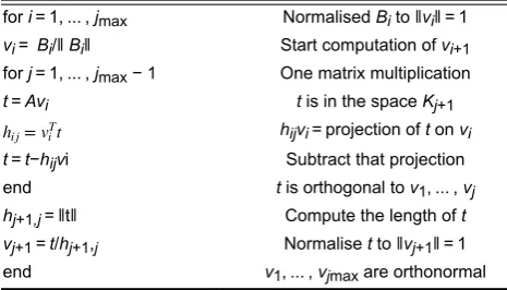
Table 1 Arnoldi's orthogonalisation

for i= 1, ... , jmax Normalised Bi to vi = 1

vi= Bi/ Bi Start computation of vi+1

for j= 1, ... , jmax − 1 One matrix multiplication

t=Avi t is in the space Kj+1

hi j=viTt hijvi= projection of t on vi

t=t−hijvi Subtract that projection

end t is orthogonal to v1, ... , vj

hj+1,j= t Compute the length of t

vj+1=t/hj+1,j Normalise t to vj+1 = 1

end v1, ... , vjmax are orthonormal

m0=E K0+p1K1+p2K2+ ⋯ +piKi−1F

m0=E(I− ( −K0−1(p1K1+p2K2+ ⋯

+p_iKi))−1K0 −1

F

(11)

For the second moment

m1= −E K0+p1K1+p2K2+ ⋯ +piKi−1C(K0

+p1K1+p2K2+ ⋯ +piKi)−1F

m1= −E K0+p1K1+p2K2+ ⋯ +piKi−1Cm0

m1= −E(I− ( −K0−1(p1K1+p2K2+ ⋯

+p_iKi)))−1K0−1Cm0

(12)

For the jth moment

mj= −

∑

∞

E−K0−1Ki ij

K0−1C pij_⋯m

j− 1⋯ (13)

Order reduction with moment matching needs moment m0 to mj be

independent on parameter series p1 p2...pi. Equation (13) shows

that the moments are combination of the matrices

( −K0

−1

(K1+K2+ ⋯ +Ki))ijK0 −1

C( −K0 −1

(K1

+K2+ ⋯ +Ki))ij− 1K0−1C

⋯( −K0

−1

(K1+K2+ ⋯

+Ki))i1K0−1C( −K0−1(K1+K2

+⋯ +Ki))i0K0−1F⋯

(14)

which means that each moment lies in the subspace spanned by the columns of the matrices in (10). These matrices are then taken to construct the projection matrix V, which is located on the first r columns of (14). This can be done by rewriting matrices A and B in Section 2 as

A= −K0−1(K1+K2+ ⋯ +Ki)B= −K0−1F (15)

m columns of the matrix B= [ B1B2…Bm] are the starting vectors

of the so-called block Krylov-subspace. The following calculation is the same with Section 1. The details of this algorithm are shown in Table 2.

3 Thermal model and simulation results

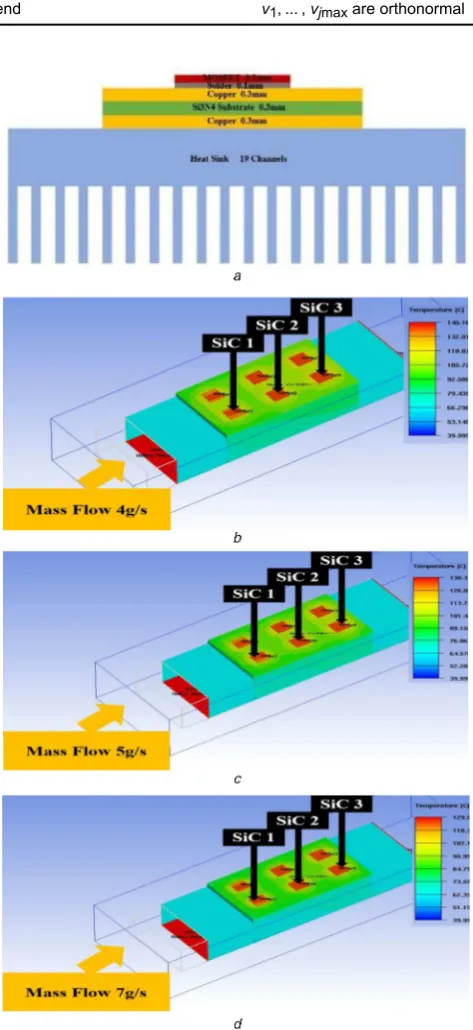
A simplified power module mounted on a parallel-plate finned heat sink is considered, as shown in Fig. 1. The power module contains six SiC MOSFETs and is assumed to be mounted on a direct copper bonded ceramic substrate and attached to the heat sinks. The boundary condition is complex due to the forced air cooling. A simplified analytical model of the heat transfer coefficient varying axially along the direction of the air flow has been established based on [22, 23]. In this paper, a dimensionless fluid dynamic entry length is introduced

Lh+= 0.0822ϵ(1 +ϵ)21 −192

ϵ π5 tanh

π

2ϵ

2

(16)

is the heat sink channel aspect ratio and

ϵ= fin thickness/channel space.

An analytical model for the Nusselt number Nu A in [23] is

suitable for the heat sink model, as follows:

Table 2 Multi-parameter Arnoldi reduction

A= −K0−1(sum(Ki)) B= −K0−1F. Block Krylov subspaces

for i= 1, ... , jmax Normalised Bi to vi = 1

vi= Bi/ Bi Start computation of vi+1

for j= 1, ... , jmax − 1 One matrix multiplication

t=Avi t is in the space Kj+1

hi j=viTt hijvi= projection of t on vi

t=t − hijvi Subtract that projection

end t is orthogonal to v1, ... , vj

h_{j+ 1,j}= t Compute the length of t

v_{j+ 1} = t/h_{j+ 1,j} Normalise t to vj+1 = 1

end v1, ... , vjmax are orthonormal

Fig. 1 Module components with heat sink (left) and steady-state thermal

Nu A= (

C4f( Pr )

Z* )

m₊

({{C1(fRe A

8 πϵγ)}

5

+ {C2C3(fRe A

Z* ) (1/3)

} 5

) (m/5)

1 m

(17)

where m is the model blending parameter provided in [22] and other parameters of (17) are given in Table 3. The Nusselt number decreases along the thermal entry length [23] and settles to a constant value. It should be noted that 0.1 < Pr < ∞ is valid for most heat exchanger applications. z* is the dimensionless thermal axial position. The friction factor Reynolds product equation (18) and (19) describes the effect of the boundary layer velocity profile on the mass transfer [24]:

fRe A= 11.8336.

V˙

Lnvair + fRe A,f d 2

1/2

(18)

fRe A,f d= 12

ϵ(1 +ϵ)[1 −192ϵ

π5 tanh(

π 2ϵ)]

(19)

With this and with Nusselt number Nu A, the heat transfer

coefficient becomes

h= huAλair dh with

d_h= 2sc

s+cands=

b− (n+ 1)t

n (20)

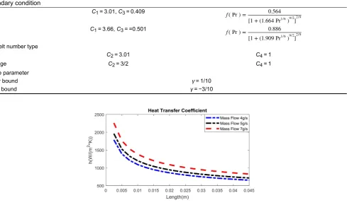
The resulting heat transfer coefficient as a function of the axial distance from the inlet for the heat sink in Fig. 1 for three different values of air mass flow is shown in Fig. 2.

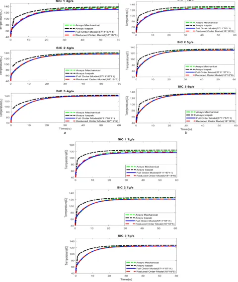
The proposed MOR is applied to the system. Figs. 3a–c illustrate surface temperature responses of the three MOSFETs identified in Fig. 1 calculated by reduced- and full-order simulation and compared to results obtained with commercial FE software ANSYS mechanical and the CFD tool ICEPAK. The ‘ANSYS mechanical’ simulations are obtained by solving the conduction heat transfer problem, removing the fins and setting the bottom baseplate surface with a convective boundary condition with heat

transfer coefficient as in Fig. 2. As can be seen, the agreement among the finite difference full order, the proposed reduced-order method and the ANSYS FE method is excellent. However, some discrepancies are present when compared with the CFD results. This is due to the approximations resulting from the semi-analytical model of the variable heat transfer coefficient. The discretisation employed in the full-order model results in a system with 5711 nodes, while the reduced order has 108 states corresponding to 18 temperature nodes per MOSFET. On the same computer and with the same mesh size, CFD takes over 300 min, the full-order simulation needs 20 min, while the reduced-order simulation only takes about 5 s.

4 Conclusion

In this paper, a novel multi-parameter order reduction is developed and applied to a power module with forced air- cooled systems. The multi-moment matching technique is used to preserve in the reduced order a number of parameters, making calculations in variable operating conditions significantly more efficient. An example of a power module cooling system with different mass air flow rates is reported.

A high degree of accuracy compared to that of conventional FE and CFD tools is shown. A significant increase in computational efficiency is demonstrated resulting in faster calculation time and memory requirements.

5 Acknowledgment

This work was supported by the European Commission Horizon 2020 – Mobility for Growth Program under Grant 636170.

Table 3 Table of coefficients for general models Boundary condition

(T) C1= 3.01, C3= 0.409 _{f( Pr ) =} 0.564

[1 + (1.664 Pr1/6₎9/2

]2/9

(H1) C1= 3.66, C3= =0.501 _{f( Pr ) =} 0.886

[1 + (1.909 Pr1/6₎9/2

]2/9 Nusselt number type

local C2= 3.01 C4= 1

average C2= 3/2 C4= 1

shape parameter

upper bound = 1/10

lower bound = −3/10

Fig. 2 Heat transfer coefficient along the axial direction of the air flow

6 References

[1] Gerber, M., Ferreira, J.A., Seliger, N., et al.: ‘Integral 3-D thermal, electrical and mechanical design of an automotive DC/DC converter’, IEEE Trans. Power Electron., 2005, 20, (3), pp. 566–575

[2] Smet, V., Forest, F., Huselstein, J.-J., et al.: ‘Ageing and failure modes of IGBT modules in high temperature power cycling’, IEEE Trans. Ind. Electron., 2011, 58, (10), pp. 4931–4941

[3] Davidson, J.N., Stone, D., Foster, M.P., et al.: ‘Real-time temperature estimation in a multiple device power electronics system subject to dynamic cooling’, IEEE Trans. Power Electron., 2016, 31, (4), pp. 2709–2719 [4] Lu, H., Bailey, C., Yin, C.: ‘Design for reliability of power electronics

modules’, Microelectron. Reliab., 2009, 49, (9–11), pp. 1250–1255

[5] Wang, W., Yuan, X.: ‘Lumped-parameter-based thermal analysis for virtual prototyping of power electronics systems’. Proc. 8th IET Int. Conf. Power Electron. Mach. Drives, Glasgow, UK, 2016, pp. 6–6

[6] Smith, G.D.: ‘Numerical solution of partial differential equations: finite difference methods’ (Oxford Clarendon Press, Oxford, 1985)

[7] Bechtold, T., Rudnyi, E.B., Korvink, J.: ‘Model order reduction of MEMS’, in

‘Model order reduction: theory, research aspects and applications’, vol. 13, (Springer, Berlin), pp. 403–419

[8] Freund, R.W.: ‘Krylov-subspace methods for reduced- order modeling in circuit simulation’, J. Comput. Appl. Math., 2000, 123, (1–2), pp. 395–421 [9] Clerk Maxwell, J.: ‘A treatise on electricity and magnetism’, vol. 2

(Clarendon, Oxford, 1892, 3rd ed.), pp. 68–73

[10] Li, Y., Bai, Z., Su, Y., et al.: ‘Parameterized model order reduction via a two-directional Arnoldi process’. IEEE/ACM Int. Conf. on Computer-Aided Design, Digest of Technical Papers, San Jose, USA, 2007, pp. 868–873

Fig. 3 Transient thermal responses

[11] Li, Y., Bai, Z., Su, Y.: ‘A two-directional Arnoldi process and its application to parametric model order reduction’, J. Comput. Appl. Math., 2009, 226, (1), pp. 10–21

[12] Li, Y.T., Bai, Z., Su, Y., et al.: Model order reduction of parameterized interconnect networks via a two-directional Arnoldi process, IEEE Trans. Comput. Des. Integr. Circuits Syst., 2008, 27, (9), pp. 1571–1582

[13] Feng, L.H., Rudnyi, E.B., Korvink, J.G.: ‘Preserving the film coefficient as a parameter in the compact thermal model for fast electrothermal simulation’,

IEEE Trans. Comput. Des. Integr. Circuits Syst., 2005, 24, (12), pp. 1838– 1847

[14] Farle, O., Hill, V., Ingelström, P., et al.: ‘Multi-parameter polynomial order reduction of linear finite element models’, Math. Comput. Model. Dyn. Syst., 2008, 14, (5), pp. 421–434

[15] Codecasa, L.: ‘Condition independent compact dynamic thermal networks of packages’, IEEE Trans. Compon. Packag. Technol., 2005, 28, (4), pp. 593– 604

[16] Bechtold, T., Rudnyi, E.B., Hohlfeld, D.: ‘System-level model of electrothermal microsystem with temperature control circuit’. Proc. 12th Int. Conf. Thermal, Mechanical and Multi-Physics Simulation and Experiments in Microelectronics and Microsystems, Linz, Austria, 2011

[17] Gunupudi, P.K., Khazaka, R., Nakhla, M.S., et al.: ‘Passive parameterized time-domain macromodels for high-speed transmission-line networks’, IEEE Trans. Microw. Theory Tech., 2003, 51, (12), pp. 2347–2354

[18] Gunupudi, P., Nakhla, M.: ‘Multi-dimensional model reduction of VLSI interconnects’. Proc. IEEE 2000 Custom Integrated Circuits Conf. (Cat. No.00CH37044), Orlando, USA, 2000, pp. 499–502

[19] Bechtold, T., Hohlfeld, D., Rudnyi, E.B., et al.: ‘Moment-matching-based linear model order reduction for nonparametric and parametric electrothermal MEMS models’, Syst. Model. MEMS, 2013, 10, July 2015, pp. 211–235 [20] Celo, D., Gunupudi, P.K., Khazaka, R., et al.: ‘Fast simulation of steady-state

temperature distributions in electronic components using multidimensional model reduction’, Package (Boston, MA), 2005, 28, (1), pp. 70–79 [21] Bechtold, T., Hohlfeld, D., Rudnyi, E.B., et al.: ‘Inverse thermal problem via

model order reduction: determining material properties of a microhotplate’, 10th Int. Conf. on Thermal, Mechanical and Multi-Physics Simulation and Experiments in Microelectronics and Microsystems, Belgirate, Italy, 2005, pp. 28–30

[22] Muzychka, Y.S., Yovanovich, M.M.: ‘Laminar forced convection heat transfer in the combined entry region of non-circular ducts’, ASME Trans., 2004, 126, (1), pp. 54–61

[23] Muzychka, Y.S.: ‘Generalized models for laminar developing flows in heat sinks and heat exchangers’, Heat Transf. Eng., 2013, 34, (2–3), pp. 178–191 [24] Muzychka, Y.S., Yovanovich, M.M.: ‘Pressure drop in laminar developing

flow in noncircular ducts: a scaling and modeling approach’, J. Fluids Eng., 2009, 131, (11), p. 111105