One and two locus inbreeding for recurrent selection and overlapping generations selection schemes : a thesis presented in partial fulfilment of the requirements for the degree of Doctor of Philosophy in Statistics at Massey University

Full text

(1)Copyright is owned by the Author of the thesis. Permission is given for a copy to be downloaded by an individual for the purpose of research and private study only. The thesis may not be reproduced elsewhere without the permission of the Author..

(2) ONE- AND TWO-LOCUS INBREEDING. FOR. RECURRENT SELECTION. AND. OVERLAPPING GENERATIONS SELECTION. SCHEMES. A thesis presented in partial fulfilment of the requirements for the degree of Doctor of Philosophy in Statistics at Massey University. Sam Choy. 197 8.

(3) ii. ABSTRACT. Inbreeding coefficients at one and two loci are evaluated for recurrent selection and overlapping generations selection schemes. These mating schemes have found great use in plant and animal breeding. The inbreeding coefficients are derived in terms of probability measures that genes are identical by descent. The procedures demonstrated here can be applied to any regular system of mating between individuals or groups of individuals.. For individual mating systems, two digametic individual measures are defined and employed in the derivation of a recurrence formula for the one-locus inbreeding coefficients. Two further classes of individual measures, trigametic and quadrigametic, are required for transition from one generation to the previous one to allow the calculation of the inbreeding coefficients for the two-locus case. This process is illustrated for the case of recurrent selection.. For. recurrent selection populations with various imposed assumptions, numerical values of the average inbreeding coefficients at the end of the breeding cycles are listed to demonstrate. the effects of linkage. and population size on the accrual of inbreeding and hence of homozygosity.. For group mating systems, gametic set measures are needed in addition to the average individual measures. Transition equations relating values in successive generations of gametic set measures are established for the calculation of the group inbreeding coefficients. As an illustration of this process, the one- and two-locus inbreeding coefficients for populations with overlapping generations are evaluated.. Both monoecious and dioecious populations of diploids. are considered. and family size is not restricted to being Poisson.. Inbreeding effective numbers found by the exact treatment here are compared to various previous approximate results..

(4) iii. ACKNOWLEDGEMENTS. I wish to take this opportunity to express my deepest gratitude to Dr B.. S. Weir for his continued patience and. inspiring guidance in supervising the preparation of this thesis.. I would also like to thank my supervisors, Professor B.. I.. Hayman and Professor A. L.. Rae for their encouragement. and valuable advice throughout the course of this work..

(5) TABLE OF CONTENTS ACKNOWLEDGEMENTS. Page iii. TABLE OF CONTENTS. iv V. LIST OF FIGURES. 1.. INTRODUCTION. 1. 2.. REVIEW OF ONE- AND TWO-LOCUS INBREEDING MEASURES. 5. 2.1 2.2 2.3 2 .4 3. 3.1 3.2 3. 3 3. 3. 1 3. 3.2 3. 3. 3 3.4 3.4. 1 3.4.2 3 . 4. 3 3. 5 4.. One-Locus Individual Measures One-Locus Group Measures Two-Locus Individual Measures Two- Locus Group Measures ONE- AND TWO-LOCUS INBREEDING FOR RECURRENT SELECTION Introduction Mating and Selection Schemes One-Locus Case Sampling Probabilities for One-Locus Case Recurrence Formulae for N�4 for One-Locus Case Recurrence Formulae for N<4 for One-Locus Case Two-Locus Case Selfing Phase Expansions for Two-Locus Case Sampling Probabilities for Two-Locus Case Intercross Phase Expansions for Two-Locus Case Discussion. Introduction Monoecious Diploids Mating Scheme One-Locus Case Two-Locus Case Numerical Results Dioecious Diploids Mating Scheme One-Locus Case Two-Locus Case Numerical Results D iscussion Inbreeding Effective Numbers for Poisson Family Sizes:. Monoecious Case. 4 . 4.2. Inbreeding Effective Numbers for Constant Family. 4.4. 3. Inbreeding Effective Numbers for Poisson Family. 4 . 4.4. Inbreeding Effective Numbers for Constant Family. I�, !,j., 5. Variance Effective Numbers. Sizes: Monoecious Case Sizes: Dioecious Case. 4.5 _,. •:. 11 11 11 14 14 16 17 18 19 23 28 33. ONE- AND TWO-LOCUS INBREEDING IN POPULATIONS WITH OVERLAPPING GENERATIONS. 4. 1 4. 2 4. 2 . 1 4.2.2 4.2. 3 4. 2 .4 4. 3 4. 3. 1 4. 3.2 4.3. 3 4. 3.4 4.4 4.4. 1. 5 6 7 9. Sizes:. Dioecious Case. Appendix: Two Gametes Per Parent GENERAL DISCUSSION. LIST OF REFERENCES. 42 42 43 43 44 49 55 57 57 58 62 73 74 74 76 79 79 81 81 87.

(6) LIST OF FIGURES Page. 3. 1. Mating and selection schemes for. 3. 2. Mating in intercross phase for minimum and maximum inbreeding. N= 4. 13. 26.

(7) 1. 1. INTRODUCTION. S i nce SEWALL WRI GHT ( 1 9 2 1 ) introduced the concept of the inbre eding coefficient F 1 i n terms of the correlation between unit ing gametes , populat i on genetici sts have found great use for such a measure as i t s ummari zes information about t h e mating sys tem.. Later , BARTLETT and. HALDANE ( 19 34 ) us ing a generat ion matri x of mating types and MALECOT ( 1948 ) us ing probabili ty arguments succeeded in provi ding alternat ive methods of calculating i nbreedi ng coefficients .. Of thes e , MALECOT's. definition of the coefficient as the probability of i dentity by descent of homologous genes within an i ndividual is more widely accepted because i t l eads to eas ier applicati on . The reason for choos i ng t h e i nbreeding coeffici ent F 1 as a bas i s for t h e analys i s of one-locus systems is partly the eas e w i t h which i t can be calculate d .. W RI GHT ( 1 9 2 2 ) gave the formula for t h e inbreeding. coefficient of an indi vi dual I in a g iven pedigree as =. l:. (_!) 2. n 1 +n2 1 + F 1 A ) ( 2. where A denot es an arbi trary common ancestor n 1 and n2 generat ions above the two parents o f I . The summation extends over all such di fferent pathways and ancestors .. For regular systems of mating ,. MALECOT ( 1 948 ) showed that recurrence formulas can be establi shed for the evaluation of the inbreeding coeffici ents . His idea was ext ended . by COCKERHAM ( 1 9 67) to include matings betw een groups of individuals . The applications of the one- locus inbreeding coefficients have been w ell studi ed ( e . g . KEMPTHORNE 1 9 57 ).. I n the first place , i t i ndicates. the effect of finite pop ulat i on s i ze or a regular system of mat ing on a populat ion o f breeding indi v i duals , thus allowing different systems to be compared.. Secondly , a knowledge o f the propert i es of the initial. p op ulation together with t he inbreeding coefficient allows the evaluation o f the mean and the variance o f a quantitative trait .. The calculat ion. o f the covariance between the genotypic values of i nbred individuals r equires the introduct i on of the four-gene WEIR and COCKERHAM ( 19 7 7 ) .. measures as discussed by.

(8) 2 Many characters of p lants and animals exh ibit continuous variation as a result of the s imultaneous s egregation of many genes at many loci affecting the c haracters .. On the other hand , a character controlled. by certa in loci may be affected by s election practis e d on other loci. The analysis o f characters in thes e s ituations neces s itates the study of multi-locus theory . While the one-locus quantitative theory involves the dependencie s between the action or frequenci es of allelic genes caus ed by dominance or inbreed ing , the cons ideration of the e ffect of two or more loci involves the further comp lications of epistas i s , linkage and linkage dis equi librium . As the analy s is of one-locus systems requires the knowledge of the inbree ding coefficient F 1 , it is natural that an analogous measure , the two- locus inbreeding coeffici ent F 1 1 should be of con s i derabl e he lp in the study of two-locus models . This quantity gives the probabi lity that two linked autosomal loci o f a diploid indivi dual carry genes i dentical by descent .. COCKERHAM and W EI R ( 1 9 6 8 ) and WEI R and COCKERHAM ( 19 6 9 a ). were able t o establish a n algorithm by which the two- locus inbreeding coeffici ent can b e calculate d and they demonstrated the procedure for sib mating and for any pe digree mating of individuals .. The algorithm. requires the introduction of trigametic and quadrigametic measures in addition to the usual dig ametic ones , the one-locus inbree ding and coancestry co effici ents needed for the one- locus theory .. WEI R and. COCKERHAM ( 1 9 69 b ) also used s imi lar arguments in conj unction with tho s e of COCKERHAM ( 19 67 ) to develop a procedure for the evaluation of two-locus group inbreedin g coeffici ents for systems of matings b etween groups of individuals . The two-locus inbreeding coefficient allows an i dentity dis equi librium to b e defined. which measures the dependence of two genes at two loci and hence increases w ith linkag e .. Thi s quantity i s zero for any p edigree mating in the ab s ence 2. o f l inkage as then the relat ionship F 1 1 = ( F1) always holds . For any regular system of mating , it i s zero for a non�inbred initial population or when complete double i dentity i s obtaine d and i s pos itive for all other generations ..

(9) 3. The two- locus inbreeding coefficient , though characteri zing the effects of linkage and mating sys tem on the identity by descent of two. pairs of l inked gen es , does not by itself provide the express ion. of j oint genotypic frequencies at two loci .. To offer complete solutions. to two- locus problems , a complete set of four�gene p arameters needs to be s et up . A pair of genes i s s ai d to be equivalent by descent if both genes descend from genes on one initial gamete .. For two g enes a , a ' at one. locus and two genes b , b' at a s econd locus , a class of individual descent measures was defi ned which gives the probab i lities of the various arrangements of thes e four genes on gametes in the initial population ( COCKERHAM and WEI R 1 9 7 3 , 1 9 7 7,. WEI R and COCKERHAM 1 9 7 3 , 1 9 74 ) .. The. measures thus relate the structure of any generation to that of an initial p op ulat ion .. A s et of eight summary components of descent mea. s ures was chos en to work with as they are simp ler to evaluate and to app ly than the original s et of measure s .. General procedures for cal. culating these summary measures have been established .. When th e structure. of the initial population i s known , these summary measures lead to express i ons for two-locus genotyp ic frequenci es and various dis equi libria funct ions , and also to the means and variances of quant itative charact ers ( WEI R and COCKERHAM 1 9 7 7 ) .. The las t pap er a lso mentioned that some. eight-gen e d escent measures would need to be defined in dealing with the problem of covariances between individuals . When two genes at each of two loci are s imultaneously equivalent by descent , their i dentity by descent is ensured .. Therefore two com. ponents o f the summary measures are the one-and two- locus inbreeding oefficients.. I n p articular , in the abs ence of ini t i al linkage dis equi. librium , these two coeffici ents are s ufficient to express the two- locus genetypic frequencies , means. and variances in terms of the propert i es. o f an initial population . Th e two- locus inbreeding coefficient t hus contains a great deal of information about the two-locus s tructure o f a p op ulation as the one-locus coefficient does for the one- locus mode l .. It is the purpose. of the pres ent work to i l lustrate furth er the evaluation of the two locus i nbreeding coefficients in the cas es of recurrent s election.

(10) 4. and overlapping generations s elect ion schemes .. These are schemes. des i gned to s low down .the rat e of inbreeding in s e lection programmes and the i nbreeding coefficients would give indications of the approach to homozygos i ty .. The literature appropriat e to the two mating schemes. w i ll be rev i ewed when they are introduced in Chapt ers 3 and 4 . Techniq ues developed for population genetics are thus being app lied to quanti tative genetics .. The mat ing schemes s tudied contain the com. plicat ion that speci fic rul es are s tated for the s election of members of a generat ion to s erve as parents of the next generation .. An indication. of the comp lexity is the fact that this thes is offers the first exact and correct evaluati on of even the one-locus i nbreeding coefficients . Just as inbre eding measures s ummari ze i nformation about mating systems , effective numbers can be defined and summar i ze the behaviour of i nbreeding measures .. S uch effective numbers will be di scussed when. appropriate throughout the thes i s ..

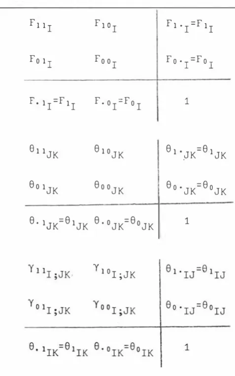
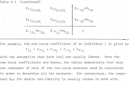
(11) 5. 2. 2.1. REVIEW OF ONE- AND TWO- LOCUS I NBREEDING MEAS URES. One-Locus Individu�l Measures For i nbree ding at one locus , the ident ity s tatus of pairs of genes. a , a ' at the locus is neede d .. [. A probability measure X wi th two compo. nents according to the identity relat ions is defined as :. =. �(a,a' ). Xl ( a , a ' ) X0 ( a , a ' ). J. r l. I� $ J. Prob ( a::a. =. Prob ( a a '. where the equivalence s i gn :: means i dentity by descent .. No res triction. is p lace d on the number of alleles. X i s a digametic measure as a and a' must be carried on two distinct gametes .. When dealing with individu al mating schemes , two types of the. measure need to be dis t inguished according to whether or not the two gametes unite and thes e two are sufficient for the es tablishment of recurrence re lations for the evaluation of the one-locus inbreeding coeffici ent : F. -I. =. -. X( a ' a '. a , a ' are o n two gametes uniting t o form individual I ). �K. =. �(a,a'. a , a ' are on two gametes taken from individuals. Evi dently , F1. 1. J. and K respect ively ) .. i s the i nbreeding coefficient of I ,. Fo i s the p anmictic coefficient o f I , 1 81. and F1 1. =. JK. i s the coancestry coefficient of J and K,. i f I is the offspring of J and K. 81 JK.

(12) 6 2.2. One-Locus Group Measures To study sys t ems of matings between groups of individuals , let. I , J , K denote indivi duals belonging to groups i , j and k respectively . Tl1e. coancestry between groups j and k i s det ermined by the iden t i ty. s tatus of genes on two gametes taken randomly from the two gametic output s ets provided by groups j and k resp ecti vely. It i s referred to as a gam etic set measure .. To take account of the gametic sampling. scheme , i t i s neces s ary to specify the groups that receive the gamet es .. 'i'.. -J k P q. =. � ( a , a'. a is on one gamete in the gametic s et that group p receives from group j and a' is o n one gamete i n the gametic s et that group q receives from group k ).. The inbree ding function of group i ,. F.,. -l. i s given by the average. coancestry between i t s parental groups , j and k say =. \}'.. -J k i i. averages taken over all such pairs of gamet es.. Recurrence relations are. then es tablished between values in success i ve generat ions of a comple t e s et of digamet ic s e t measures for the evaluat ion o f F .. l. A difficulty arises when one group acts as a donor of both gamet es for a gametic set measure , for example 'i'. . The two gametes t aken Jp]q from the same group may have come from the s ame indivi dual and t h ere i s .. a pos s ibility o f t h e two genes being automatically i dentical by descent. This s i t uation proh i b i ts the expansion of gametic set measures back directly to gametic s et measures of the previous generat i on.. I ndivi dual. measures need to be defined to i dentify cas es t hat the two gametes of intere s t have come from the same or two distinct individuals : =. X ( a , a'. a i s on a gamete taken from individual J i n group j and a' i s o n a gamete from individual K in group k ) ..

(13) 7. Primes are used to denote distinct individuals . For example, the average individual coancestry function for two distinct members of group j is written as � .J !·' The procedure is thus to express a gametic ·. J. J. set measure as a linear combination of individual measures by using the gametic sampling p robabilities, and then to expand these individual mea sures back to gametic set measures of the previous generation ( WEIR and COCKERHAM 1 9 6 9 b ) . Two - Locus Individual Measures. 2.3. The following work serves as an extensi on of Section 2 . 1 and is based on the work of WEIR and COCKERHAM ( 1 9 6 9a ) . For two loci with genes a and b respectively, the identity status of two pairs of genes, a, a' and b, b' is needed . The usual procedure is to define a four component vector for these gene pairs as. X ( ab,a'b' ). =. X 1 1 ( ab,a'b' ) X 1 0 ( ab ' a'b' ) X01 ( ab,a'b' ) X00 ( ab,a'b' ). =. Prob ( a::a', Prob( a::a', Prob ( a$a', Prob ( a$a',. b::b' ) b$b' ) b::b' ) b$b' ). To evaluate such tWo-locus inbreeding measures, it is necessary to distinguish the cases where the pairs of genes are carried on two, three or four gametes . There are two digametic measures, just as there are in the one-locus case : FI. �K. = � ( ab,a'b'. =. ab,a'b' are on the two gametes uniting to form individual I ) ,. � ( ab,a'b'. ab,a'b' are on two gametes taken from individuals J and K, respectively ) .. The trigametic and quadrigametic measures are written as land �' respectively : = � ( ab,a'b' Yr·JK '. ab, a�b' are on three gametes taken from individuals I, J, and K, respectively) ,.

(14) 8. s. � IJ ; KL. = _X ( ab , a ' b'. a , b , a' , b' are on four gametes taken from. indi vi duals I, J, K and L, respe ct1vely ) .. The four components of each meas ure s um t o uni ty .. The fi rs t and. fourth component of �I' giving the probabi li ti e s of doub l e identi ty and doub le non- i denti ty by des cent are termed the two- locus i nbreedi ng and panmi ct i c coeffi ci ent s respectively for indi vi dual I . One locus measures may be found by summi ng appropriate components of two- locus meas ures as shown in Table 2 .1.. Table 2 .1. Re lations hip between One- and Two- locus Measures F 1 1I. F1 OI. F1 'I =F 1I. Fo1I. Fool. F o.1=F o1. F. 1I=F1I. F.oi=Fo i. e 11JK. 81oJK. 81 ' JK =81 JK _. 8o1JK. 8ooJK. 8o. JK =8oJK. 8.1 K=81JK 8 .oJK=8oJK J. y 1 oi. JK '. 1. 1.

(15) 9 ( continue d ). T able 2 . 1. 611IJ· KL '. 61oiJ;KL. e1.IK=e1IK. Oo1IJ K · L. .. OooiJ ·KL. 8o.IK =8o iK. 8.1J =81J L L. 8 .o J =8o J L 1. '. '. 1. For examp le , the one- locus coefficient of an individual I F1I = F 11I +. F1 OI = F11I. +. Fo1I. with the as sumpt i on that both loci are equally inbred .. lS. given by. Once the. one- locus coeffi cient s are known , the tables demons trat e that only one component of each of the two- locus measures need be calculat ed in or der to determine a l l the measures .. For conveni ence , the compo. nent Xoo for doub le non- i dentity i s usually chosen to work w i th . The linkage p ar amet er i s defined so that the gametic array pro duced by an individual with genotype ab I a'b '. 2.4. lS. :. Two- Locus Group Measures I n analys ing group mating sys t ems at two loci , WE I R and COCKE RHAM. ( 19 69b ) have define d t hre e c las s es of game t i c set measures :. �. k = � ( ab , a'b ' J P q. ab are on one gamete in the gamet i c s e t that group p receives from group j and a ' b' are on one gamete in the gametic s et that group q receives from group k ) ,. V· l. ·] k P' q r •. =. � ( ab , a'b '. ab is on one gamete i n the game t i c s e t that group p receives from group i , a' is on one gamete in the game t i c s et t hat group. q. rece ives from group j and b ' i s. o n one gamete i n the game t i c set that group r receives from group k),. M. • - ·r .. ··••llT:.!TY. t;;·"i.�.x.

(16) 10. s -i j •k £ p q' r s. =. _X ( ab , a ' b '. a , b , a ' , b ' are on four gametes in the game t i c s ets that groups p ,q , r , s receive from groups i , j , k , £ , respect ively ) .. The p ro cedure for the evaluation of the two- locus group inbreed ing funct ion F . i s to firs t express i t as the coancestry function between -l. the parental groups , j and k s ay , F.. -l. =. �. j .k. l. l. and then to estab lish re curren ce relations for a comp lete s et of gamet i c s et measures for the calculation o f �- k . J i i J us t as in the one- locus cas e , whenever a group appears more than once as a donor in the subscript of a gamet i c s et measure , the exp an s i on procedure requires an intermed iate stage of individual measures . Let I , J , K , L denote members of group i , j , k ,t , resp e ct ively , three types of indi vi dual measures are distinguished : ab , a ' b ' are on two gamet es t ak en from indivi duals J , K in groups j and k , resp e ctively ) , yI. -. l .. ;. J .K J k. =. � ( ab , a ' b '. ab , a ' ,b ' are on thr e e gametes taken from individuals I , J , K in groups i , j and k , respe ct ively ) , a , b , a ' , b ' are on four gametes taken from individuals I ,J , K ,L in groups i , j , k and i, respect ively ) ..

(17) 11. 3. ONE- AND TWO-LOCUS I NBREED ING FOR RECURRENT SELECT I ON I ntroduction. 3.1. With the inbreeding measures defin ed generally , and the machinery deve loped by COCKERHAM and W E I R ( 1 9 6 8 ) for the cal culation of the two locus inbreeding coefficients , in this Chapt er a one- and two - locus analysis of inbreeding for a population undergoing recurrent s election is presente d . The use o f recurr ent s el ection ( RS ) procedures i n p lant b reeding is now wel l es tablished .. As PENNY , et a l ( 1 9 6 3 ) point out in th eir. review� the recombination or cro s s ing phas e in an RS programme s lows the rapid approach to homozygosity which limits s election under s elfing sys tems .. To monitor the level of homozygosity in RS programme , it i s. convenient to calculate inbreeding coeffi cients .. These coeffi cients. indicate identity by des cent and so do not give a complete des cription of homozygosity .. They do provide lower bounds , however , ( CA I N and. H INKELMANN , 1 9 7 0 ) and the algebra needed to estab lish rec1�rence equations for inbreeding coeffi cients may also b e applied direct ly to measur es of homo zygosi ty . A one- locus coeffi cient was cal culated by SPRAGUE , et al ( 1 9 5 2 ) and a quite detailed di s cussion o f one- and two- locus coefficients was given by CAIN and H I NKELMANN ( 1 97 0 , 1 97 2 ) .. These last two papers. cont ain s ome errors and do not seem to follow the mos t natural deve lop ment of inbreeding meas ures .. One difficulty with the papers of CAIN. and H INKELMANN is that they are base d on the approach of S H I KATA ( e . g . , SHIKATA� 1 9 6 5 ) which is of limited application ( e . g . , W E I R , 1 971 ) .. Mating and S e le ction S chemes. 3. 2. The population consis ts of diploid individuals capable of both selfing and inter crossing . allele s. There is no restriction on the number of. at each of the loci s tudied . A const ant number of progeny per. indivi dual is as sumed and p o s sible viabi lity effects are ignored .. The. development will b e bas ed on one progeny per mating ( self or intercros s ) ..

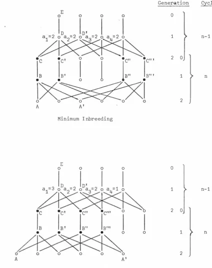
(18) 12. I n i ti ally N non- inbred and unr e lated individuals are drawn from a s ource populat i on and s e lfed .. The result ing N offspring are crossed. in -all pos s ible pairs and then another selfing phase ent ered .. The. populat ion s i z e would quick iy become unmanageable of course for there would be M. =. N ( N - 1 ) / 2 i ndivi duals at the end of the first i ntercross. ph as e , M ( M- 1 ) / 2 at the end o f t he s econd , and so on . S election will be supposed t o be practi s ed by s e le ct ing N indivi duals at the end of each s elfing phas e . · The bas is for this s ele ct ion wi l l not be d i s cussed , but note ( CA I N and HINKELMANN , 1 970 ) that this treatment includes such s chemes as s impl e RS, reciprocal RS and RS for general and s pecific combining abi li ty .. The calculati ons made will. i nc lude a ll of the M individuals at the end o f each intercross phas e . S election wi l l be s upposed t o be at random , so tnat i t is necessary to mak e us e of sampling probab i l i t i e s .. Any mat ing s cheme in which there. i s no choice of mates is expres s ly exc luded from cons i derat ion here , but may be analysed by other methods ( e . g . , WEI R and COCKE RHAM , 1 9 6 9a ) . !1ost of the discussion w i l l b e for the cas e where N individuals are chosen quite at random from the M at the end of each s elfing phase , and so would be appropr i at e for a control populat i on .. Following. CAIN and H I NKELMANN ( 1 970 ) , two s chemes of random s e lection with c on s traints will be cons i dered . " maximum" inbreeding s cheme s .. Thes e are the so called "minimum" and I n the former case , each of the s elected. i ndivi duals contr ibut e s exa c t ly two gametes to the next group of s e le cted i ndividuals .. In the latter cas e , one of the sele cted individuals contri . butes N - 1 gametes , two contribute two gametes whi le t he rema ining N - 3 individuals each contr ibutes e xact ly one gamete to the next group o f s e lected individuals . for N. =. The mat ing and s e lect ion s chemes are i llustrated. 4 in Figure 3 . 1 .. Random s election is when the four individuals. s elected in generation 1 o f a cycle are s e le cted without regard to game t i c contributions in th e previo us cyc le . The quant ities t o b e determined are the average inbreeding coeffi c i ents for the intercross and s e lfed populations , so that all members o f these populations mus t b e considered whether or n o t they contribute to s u cceeding generat ions ..

(19) 13 Gener«tion. Cy cle. 0. 0. •. B. I. 0. A. 0. 0. •. 0. 0. 0. 0. 0. B'. A'. 1. �. I: :. •. 2. c"'. B" '. n- 1. 0 1. •. 0. n. 2. Minimum I nbreeding. E. 0. • c. 0. •. B. 0. c". B". 0. • "' c. B"'. •. •. 0. 0. 0. 0. 0. 1. �. 0. 0. 0. 0. �. 2. n- 1. 0. 1. 0. 2. A'. Maximum I nbreeding. Figure 3 . 1 .. Mating and sele ction s chemes for N. =. 4.. indivi duals are shown as solid circles .. S e le cted. n.

(20) 14. 3. 3. One- Locus Cas e The inbree d ing coefficient of a random on e of the M members, say. A, o f generat ion 2 ( int ercro s s e d generation ) of cy cle n can be written As not a ll members of th i s generat ion have the as F1 o r as F 1 A ( 2,n )" s am e p e d igree, F 1 i s an average measure . F 1 lS f irst expressed as A A , the coancestry of two of the N dist inct individuals B and B' 81 BB' chosen at random from gen era t i on 1 ( s elected s e lfed generat ion ) of The p rocess of tracing game t es back in t ime cont inues unt i l. cyc le n .. a s et o f tran s i t i on equations. lS. established wh i ch allow the calcula. t ion of F 1 and of F 1 . B A. Samp ling Probabilities for One- Locus Cas e. 3. 3 . 1. I f C and C' are the pare nts o f B and B', respective ly, they are d i s t inct members of the s e lect ed int ercro ss populat ion ( generat ion 2 o f cycle n- 1 ) and (3.3.1) The s elected int ercross population refers to the parent s of the s el ected s e lfed populat ion .. Further expansion back in t ime requires. a ccount to b e taken of whether C and C' have a common parent, with probabil ity P probab i l i ty P. 21 1. , or whether they have four dist inct parent s, with. . For both s chemes in Figure 3 . 1, individual A has 1111 grandparent s C, C' with a common parent D, wh i le the grandparents of i nd ivi dual A' do not have a common p arent .. I n general, when a set of. 2m gametes recei ved by m members of generat i on 2 o f cy cle n i s cons i dered, P. i s the probabi l ity t hat the s e gametes are from r .t t t 1 2·· r indi viduals in generat ion 1 of cyc le n and that the ith of these individuals contribut ed t . of the gametes . l. Thi s requires that the. t . s um t o 2 m . l. The four gametes received by d ist inct indiv i duals C, C' neces sarily come from three or four individuals un less N , the s e lected populat ion s i z e, i s equal to 2 . p. 211. + p. 1111. =. Thi s provides 1' N. �. 3;. P. 22. =. 1, N. =. 2..

(21) 15 For the unrestricted ran dom samp ling s cheme , N. �. 3 , the s ampling. probab i lities may be taken to refer to four gametes uniting to form any two of the M cros s ed offspring in g eneration 2 of a cycle . The M number of such pairs of offspring i s ( ) and , sin ce s e lection i s 2 random , the number of ways in which t hr ee dist inct parents can b e chosen for a pair i s (U) Finally , the number o f ways in whi ch one 3 of the three parents can be chos en to contribute two gametes , and 3 become the common parent to t he p air of individuals , l S ( ) s o that 1 p. 1111. =. N- 3 , N N+ 1. �. (3.3.2). 3. For the restricted random s elect i on s chemes , as in CAI N and H I N KEL MANN ( 1 97 0 ) , let a . denot e the number of gametes contribut ed by l. the i th s elected indivi dual to the next generation of s elect ed i nd i vi duals . 1. Thes e a . must s at i s fy l. �. N. a. � N - 1. L. l. i=1. a . = 2N l. and may be regarded as the number o f gametes the ith s elect ed s elfed individual contribut es to the following generation o f s elected inter c an be regarded as the prob ab i l i ty that 211 a p air of individuals from the s ele cted intercross populat ion have a N common parent in the preceding s ele cted s e lf populat ion . There are ( ) 2 s uch pairs of individuals and L a . ( a . - 1 ) / 2 p airs of gametes from a l l i s ingle parent , so that cros s ed indiv iduals .. Now P. = L a . ( a . - 1 ) / N ( N- 1 ) l l i Figure 3 . 1. s hows. l. p. 211. = 2/ ( N- 1 ). the a . 's for the cas e N = 4 . l. =. i nbreeding , a . = 2 for i N. ( 3. 3. 3). 1 , 2 , . . . N s o that �. 3. whi le for maximum inbreeding i t is appropriate to write a a. 2. = a P. 3. = 2, a. 211. i. For minimum. = 1 for i = 4 , 5 , . . . N and hence. 2 = (N - 3N+ 6 ) /N ( N - 1 ). N. �. 4. •. 1. = N-1 ,. ( 3 . 3. 4).

(22) 16. Note that , a s e xp e ct e d , P. for unrestr i cted random s ele ct ion i s 211 greater than that for minimum inbreeding and less than that for maximum inbre eding for a l l N. 3. 3. 2. �. 4.. Recurrence Formulae for N. �. 4 for One- Locus Cas e. I f primes are us e d to denot e dis t inct random individua ls , equat ion ( 3 . 3 . 1 ) can be e xpressed as ( 3. 3 . 5) From the usual result for the coancestry of an individual with i ts e lf 8 1 DD = ( 1 + FlD ) / 2 FlD = 8 1 EE. =. ( 1 + Fl ) / 2 E. ( 3. 3.6). and these express ions may be subs tituted into ( 3 . 3 . 5 ) whi ch , with 8 1 DD' wri t ten as F 1 , gives C ( 3. 3.7) Re cal l that D , D' are any two of the s e lected s e lfed individuals , wh i le C in F 1 refers to any of the M offspring obtained by crossing thes e . C I n general t hen , the average inbreeding for t he whole of the int ercros s generation. follows from ( 3 . 3 . 7 ) as. 1 1 6 + ( 1-P Fl /4)F 1 3p ( 2 ,n) = ( 2 , n- 1 ) 211 211. + p. 211. Fl. ( 2 , n- 2 ). / 16. and that for the whol e of the s e lfed generat ion. ( 3. 3. 8). follows from ( 3 . 3 . 6 ). as F1. (1,n). = ( 1 + Fl. )/2 ( 2 , n- 1 ). ( 3 . 3. 9 ). Whi l e any initial conditions at all may be a ccommodated , it is usual to t ak e F 1 = F1 is for t h e init i a l N = 0 , where F 1 ( 2, 0) ( 2,0) ( 2, 1) in dividuals ..

(23) 17. For unrestri cted r andom s ele ction , substitution of P ( 3 . 3 . 2 ) into ( 3 . 3 . 8 ) gives F1. ( 2 ,n ). =. 211. . 3 1 N F + + -- F 1 ( 2 , n- 1 ) 4 ( N+ 1 ) 1 ( 2 , n-2 ) N+ 1 4 ( N+ 1 ). ...,._..--;' ,..,...,.. from. ( 3 . 3 . 10). which .corrects equations ( 3 . 1 ) , ( 3 . 2 ) of CAIN and H I N KE LMANN ( 1 97 0 ) . from ( 3 . 3 . 3 ) is s ub s tituted For r es tri cted r andom s election , if P 211 into ( 3 . 3 . 8 ) , a res ult � s obtained similar t o that in equation ( 6 . 1 ) of CA IN and HINKELMANN ( 1 970 ) , who refer to this case as effective dir e c tional s e lection . I n t he maximum inbre eding case ther e is the unusual result t hat average inbre eding increas es with population size . for N. �. This is becaus e ,. .6 , P. is an in creasing function of N . As N incr e ases , there 211 is a gre at er chance that any two members of the s el e cted inter cross gener ation have a common parent .. This extreme cas e is less likely to. o ccur by chance under unrestrict ed r andom selection as N incr eas e s , however .. 3.3. 3. Re curr en ce Formulae for N. <. 4 for One- Locus Cas e. For a population t o be maintained at si ze less than four , there can b e no s election since M. $. N and the situation is r eally out si de. the s cope of thi s Chap t er . For N = 1 the sy stem becomes the simp le s elfing cas e with no s cop e for int er crossing .. For N = 3 each indivi dual a lway s. contrib utes exact ly t w o gametes to succeeding gener ations , and , from either ( 3 . 3 . 2 ) or ( 3 . 3 . 3 ) , P F1. ( 2,n). 211. = 1.. E quation ( 3 . 3 . 8 ) does reduce t o. - _]__ + � F 1 + _!_ F 1 16 4 ( 2 , n- 1 ) 16 ( 2 , n- 2 ). _. ( 3 . 3 . 11 ). as given in ( 6 . 1 ) of CAIN and H INKELMANN ( 1 970 ) . To maintain a p opulation of size N = 2 , it would b e neces s ary for th e pair of indivi duals in each inter crossing phas e to leave two off spring inst ead of one .. The system then r educes t o one of alternating. s el fing and ful l sib mating , for which the appropriat e r e curr ence.

(24) 18. formula is 3 F l( 2 , n ) = 8. +. 1 1 F F + 2 1 ( 2 , n-1 ) 8 1 ( 2 ,n- 2 )". ( 3 . 3 . 12). Equat ion ( 3 . 3 . 9 ) is still t9 be used in conj unction with ( 3 . 3 . 1 1 ) and ( 3 . 3 . 1 2 ) . Two-Locus Case. 3. 4. For inbreeding at two loci , the identity status of two pairs of genes , a ,a' at one locus and b , b' at anot her locus needs to be consi dered . The four genes may be carried on two , three or four distinct gametes and hence , in addition to the digamet ic measures sufficient for the one-locus analysis , two further classes of measures� trigametic and quadrigameti c , are required for transition from one cycle to the previous one to allow the calculation of the two-locus inbreeding funct ion . From Table 2 . 1 , it is evident that , to determine the four com ponents of the inbreeding function , the only information needed is one of the components in addition to the one-locus coefficients , as for example , F11= F00 + 2F 1 - 1 . It will be convenient to work with the two-locus panmictic coefficient , and the corresponding ( fourth ) components of other measures . For further convenience +. the. following average measures are defined. ) 2 r.I·KJ /. =. C:ti · JK. iiJ ; KL. =. ( .§_. IJ·KL + .§_IJ ; LK ) / 2. 0IJ ·, KL. =. ( .§_. IJ · KL + .§_IJ· LK. y I ·JK '. '. '. '. '. '. +. � I ; KL. +. � I·LK ) / 4 '. Expansions of two-locus measures mak e use of the linkage parameter A which was defined on Page 9 . The one�locus situation corresponds to.

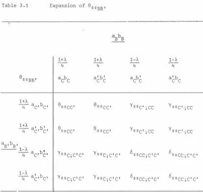
(25) 19 A= 1 , for then the two loci are completely linked and a and b are transmitted as one gene . Independent transmission of a and b occurs when A=O .. 3.4. 1. Sel fing Phase Expansions for Two - Locus Case. The general method of calculating I for any generation follows that for the one-locus coefficient F 1 • Starting with a random member A of generation 2 of cycle n , � is expressed as the two-locus coancestry coefficient of its distinct parents (3.4.1) The tracing of the genes received by A back through the selfing phase is now more complicated since the four genes may be carried on two , three or four gametes in that phase. In particular , if indivi dual B receives gametes acbc , a �b � from its single parent C and trans mits gamete �bB to individual A, then aBb B is traced back to the array. and similarly for the gamete transmitted from B' to A. The two arrays may be written as the margins of a two way table , as in Table 3 . 1 , and the value of 800BB' in each of the sixteen cases written in the body of the table . Collecting terms ln this table shows that =. ( 1+ A ) 2 1 -A 2 + -8 0°CC' 4 2-- Yo o c;C'C'. ( 3 . 4. 2 ). where , once again , primes are used to denote distinct rather than particular individuals ..

(26) 20 Table 3 . 1. Expansion of. 1+4 1... 1 +1.. 4. 1 +1.. 4. 1+1... 1-1... 1-4 1... a'b' c c. acb' c. a'b c c. 4. 4. eoocc'. Boo. cc•. Y 0°C';cc. Y 0°C1;cc. b' a' C1 C 1. eooccl. e ooccl. Yooc•;cc. y 00C I;cc. Yooc;C'C'. Yooc;C'C. I. 6oocc;C1C'. 0oocC;C1C1. Yooc ·c lcl '. Yooc;C'C'. 0 00CC;c I c I. 0 0°CC;C1 C'. -. 4. BB '. ac,bc,. a ,b I B B -1.. 1 4- a b cl � , 1- 1... 8 00. �. a lb c,. Further expansion , now through the intercross phase , will require the use of sampling probabilities as previously , followed by expansions through another selfing phase . These selfing expansions will evidently be for genes received by two , three or four individuals ( in generat ion 1 of cycle n- 1 ) ..

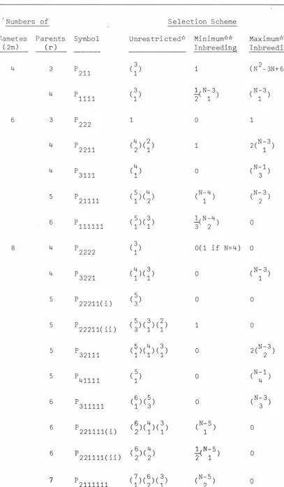
(27) 21 For the other digametic measure 800BB ' double non- identity is preserved only if the four genes on the two gametes from B descend from four distinct genes on the two gametes received by B from its single parent c: This occurs wi th probability ( 1+A 2 ) / 4 and hence ( 3. 4. 3) When genes a' , b' , or when all four genes a , b , a' , b' , are on separate gametes from B , double non-identity is preserved with probability 1 / 4 and ( 3 . 4 . 4) Y o o B ; BB 1 = 4 8 o o cc .. ( 3. 4 . 5). The argument for the expansion of Y o o B · B'B' lS the same as that ' for 800BB' except that the frequencies for the gametic array of a' b' are all equal to 1 / 4 . Since genes a' , b' are on separate gametes , linkage cannot affect these frequencies . The appropriate expansion is then 1+A 1 Y o o B B' B' = 4- 8 o o cc' + 2 Y o o c ; C'C' · '. --. +. 1-A 4 0 0 0C C ; C C I. ( 3.4.6). I. When genes a and b are also on separate gametes , link age does not affect the gametic arrays of either ab or a' b'. The expansion for 000BB B'B' is then obtained from ( 3 . 4 . 6 ) by removing A '. 1 1 1 = 4 80°CC' + 2 Y o o c ; C'C' + 4 8 o o cc ; c'c'· ( 3 ·4 · 7 ) To preserve double non-identi ty in expanding y00B·BB' , genes a and a' must be traced back to genes on distinct gametes received by B from C so that 1 ( 3.4. 8) Y o o B ; BB' = 2 Y o o c ; CC' '. By symmetry the expansion for Y o o B·B'B is ' 1 = 2 Y o o c ; C'C. (3.4.9).

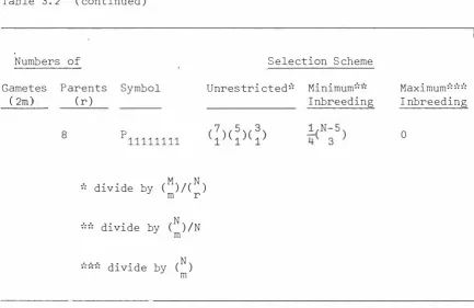
(28) 22 Combining equations ( 3 . 4 . 8 ) and ( 3 . 4 . 9 ) leads to the expansion of the following average measure 1. .. ( 3 . 4 . 10 ). = 2 Y o oc ; CC'. Consider the expansion of y the gamete carrying ab may 00B;B'B"' be a paren tal type or a recombinant type with probabilit ies ( 1 +A ) / 2 or ( 1- A ) / 2 respectively . Therefore y 00B ;B I B". 1+ A = 2-. y00c ; c I C". 1- A + 2-. 000 cc ; c I C". ( 3 . 4 . 11 ). When genes a , b are carried on separate gametes , A may be removed from equation ( 3 . 4 . 11 ) giving 1. 1. + 2 ° 00cc ; c I C" = 2 y 00c ; c I C". 'B" 000BB·B '. ( 3 . 4 . 12). For 000BB'·BB" genes a and a' must be traced back to genes on two gametes received by B to preserve double non- ident i ty . This occurs with probability 1 / 2 since a and a' are on separate gametes and hence '. ,. 1 = 2. ° 00cc I. ; CC". ( 3. 4 . 13). By symmetry =. 1 2. ° 00c I c ; C" c. ( 3 . 4 . 14 ). When the same argument i s also applied to genes b and b' , the following expansion is obtained ( 3.4.15) Equations ( 3 . 4 . 1 2 ) - ( 3 . 4 . 14 ) provide the expansi on of the average quadrigameti c measure ( 3 . 4 . 16 ) F inally. 6. OOBB' ;B"B'". =. 0. ooCC' ; C"C'". ( 3 . 4 . 17 ).

(29) 23 These equations may be manipulated more easily in matrix form . For the selfed generation of cycle n , the twelve measures needed can u ( ,n ) be written as a vector 1 �C 1 , n ) =. 8 [eOOBB ; ooBB' ' Y ooB;BB ' Yoo B;B'B' ' YooB;BB' '. and the ten measures needed for the intercross generat ion of cycle n- 1 are written as -( v 2 ,n- 1 ) or as v r O , n ) -v' � 2 , n - 1 ) = [ e oo_ cc. y 0 0 c ;c I c I. 6oocc;C'C' ' 6oocc' ;CC'. ' y 0 0 c;cc I. ' y 0 0 c;c I C". 6oocc;C'C". 0 0 0 cc I ' C" C"' J . •. Equations ( 3 . 4 . 2 ) - ( 3 . 4 . 7 ) , ( 3 . 4 . 1 0 ) - ( 3 . 4 . 1 2 ) and ( 3 . 4 . 1 5 ) - ( 3 . 4 . 1 7 ) become ' ( 3 . 4 . 18 ) � 1 , n ) = '¥� ( 2 ,n- 1 ) = '* �o , n ) where the 1 2 x 10 matrix '¥ has elements defined by those equat ions .. 3.4. 2. Sampling Probabilities for Two-Locus Case. The previous section showed t hat account must be taken of gametes received by two , three or four individuals in generation 1 of a cycle . The four genes of interest on these gametes can be traced back to genes on up to four gametes received by individuals in generation 2 of the previous cycle . Sampling probabili ties are needed for these intercross gametes . To take proper account of the restrictions on mating in the intercross phase, sampling probabili ties are defined forilll 2m gametes received by m individuals ( m = 2 , 3 , 4 ) . Appropriate sums of these pro babili t i es are then taken to give the required probabilities for up to four gametes . The sampling probabiliti es are given in Table 3 . 2 ..

(30) 24 Gametic Sampling Probabilities. Table 3 . 2. Numbers of. Selection Scheme. Gametes Parents Symbol (r) ( 2m ) 4. 6. 8. t. 3. p. 4. p. 3. p. 4. p. 4. p. 5. p. 6. p. 4. p. 4. p. 5. p. 5. p. 5. p. 5. p. 6. p. 6. p. 6 7. p. p. Unrestricted•'•. Minimum•';;': Inbreeding. Maximum•'••'>•'• Inbreeding. 211. (3) 1. 1. ( N 2 - 3N + 6 ) I 2. 1111. (3) 1. 1:_ ( N- 3 ) 2 1. ( N-3 ) 1. 1. 0. 1. 2211. (4 ) ( 2 ) 2 1. 1. 2(N-3 ) 1. 3111. (4) 1. 0. ( N- 1 ) 3. 2 1 1 11. ( 5 ) (4 ) 1 2. ( N- 4 ) 1. ( N- 3 ) 2. 111111. ( 5)(3) 1 1. �N-4 ) 3 2. 0. 2222. (3) 1. 0( 1 if N = 4 ). 0. 3221. (4)(3) 1 1. 0. ( N- 3 ) 1. 22211( i ). ( 5) 3. 0. 0. 2221 1( ii ). ( 5) ( 3) (2) 3 1 1. 1. 0. 321 1 1. (5 ) ( 4 ) ( 3 ) 1 1 1. 0. 2 (N-3 ) 2. 411 1 1. ( 5) 1. 0. (N- 1 ) 4. 311111. (6) (5) 1 3. 0. ( N- 3 ) 3. 221 1 1 1 ( i ). (q) ( 4 ) ( 3 ) � 1 1. ( N- 5 ) 1. 0. 2 21 1 11 ( ii ). ( 6)(4) 2 2. �N- 5 ) 2 1. 0. 2111111. ( 7) (6) ( 3) 1 2 1. ( N- 5 ) 2. 0. 222.

(31) 25 Table 3.2. (continued). Selection Scheme. Numbers of Gametes ( 2m). Parents. Symbol. 8. p111111 1 1. (r). Unrestricted'". Minimum•'n';. Inbreeding. Maximum�':-.,':�':. I nbreeding. 0. M N ' d' 'de by ( )/ ( ) '' 1v1 r m N '"'"divide by ( )/N m N ,..,,.,.,divide by ( ) m. tAssumes that N � r in any line and that N � 4 .. The derivation of the sampling probabilities in Table 3.2 is i llustrated by reference to P , 21111. the probability that the six. gametes received by three of the N selected members of the intercross generation descend from five members of the selected self generation in the previous cycle in such a way that one of the five gives two gametes.. F or the unrestricted random selection case, the six gametes. c�nsidered are. received by any three of the M members of the whole. intercross generation so that P will have a denominator of (�). 21111 ,. F or the numerator. note that there are (�) ways of choosing the. five members of the self generation and (�) ways of choosing one of them to give two gametes.. 4 There are then ( ) ways of choosing two 2. from the remaining four individuals to provide the gametes which unite with the two from the first individual chosen and so. =. 0 .. N �. 5. N <. 5.

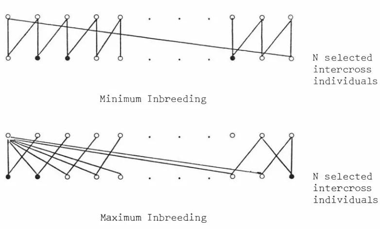
(32) 26 Although expressions were provided b y CAIN and HINKELMANN. ( 1 970 ) ,. it is not possible to express the probabilities for the restricted selection schemes in terms of a ' i. the numbers of gametes contributed to. the selected intercross individuals by the ith selected selfed individual. When the probabilities involve a choice of more than one member of the self generation (in contrast to the one needed for P in the one211. locus case),. knowledge of the mating pattern between members of this. generation is needed.. A. Such knowledge is not provided by the a .. l. .. restriction not m entioned by CAIN and HINKELMANN is made in the. case of minimum inbreeding. inbreeding scheme,. in the intercross phase,. mating (KIMURA and CROW, e xample,. It will be assumed that the minimum. 1 9 63N. is equivalent to circular. for N individuals.. This means, for. that it is not possible to select two sets of N/2 offspring. that have disjoint sets of N/2 p arents.. The sampling probabilities P. 21111. for the two restricted selection. schemes will be derived with reference to the three selected intercross individuals as indicated by solid circles in Figure. 3 . 2.. In each case,. these three individuals receive six gametes satisfying the definition of. p21111". N selected intercross. individuals Minimum Inbreeding. N selected. intercross. individuals. Maximum Inbreeding. Figure. 3. 2.. Mating in intercross phase for minimum and maximum inbreeding..

(33) 27 For either restricted selection scheme three intercross individuals. N can be chosen 1n ( ) ways. 3. In the minimum inbreeding case. twQ of these three can be chosen to have a common parent in N ways. The third can be chosen not· to have a parent in common with either of the first two in (N-4) ways so that. p 1111 2. �. =. N(N-4)/( ). N �. 5. =. 0. N < 5. In the maximum inbreeding case the common parent for two out of the selected intercross individuals must be the selfed individual which contributes (N-1) gametes.. Two out of these (N-1) gametes. must unite with gametes from the two selfed individuals which con tribute two gametes , which means that the two selected intercross individuals with a common parent can be chosen from (N-3) such indivi duals.. is specified is then The third individual for which P 21111. determined and. p 1111 2. =. =. N-3 N )/( ) ( 2 3. 0. N �. 5. N <. 5. The notation for the sampling probabilities in Table 3. 2 has been extended in two places to prevent ambiguities. P. 22211 (ii). 22211(i). and. are used according to whether or not each of the three indivi. duals giving two gametes mates with the other two. and P. P. 221111(ii). Similarly P 221111(i). distinguish the cases of whether or not the two. individuals giving two gametes mate.. In Table. 3.2 also , and for the remainder of this Chapter , attention. will be restr�cted to the case of N � 4.. When sampling probabilities. involve gametes from r parents , it is assumed that N � r , that the probability is zero if r >N.. or.

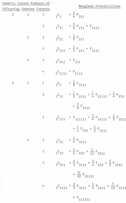
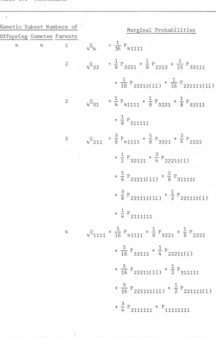
(34) 28 3. 4. 3. I nt ercross Phas e Exp an s i ons for Two- Locus Cas e The intercross phase exp ansi ons amalgam ate two steps .. After. exp anding through the s elflng phas e of cy c le n , a s e t of measures was obtained involving gametes from members of t he int ercross v -( 2 , n- 1 ) generat ion of the previous cyc l e . These gametes must first be related to gametes received by that intercross generation and then to gametes from the. preceding s elf generation ( i . e . , to u. ( 1 , n- 1 ) The first s tep takes account of re combinat i on and the s econd step. ).. of game t i c s ampling. The s i mplest exp an s ion i s for the digametic meas ure. 9 00cc·. Double non- i dentity can b e maintained only i f the four genes on the two gamet es from C descend from four d i s t inct gene s on two gametes 2 received by C . This occurs wit h prob ability ( 1+A ) / 4 and these last two gametes necessarily des cend from dist in ct individuals D , D' so that 2 1+1.. -4- 9 D 0 DD'. =. lS. ( 3 . 4 . 19 ). The two gametes for wh i ch the other digamet i c measure 800 CC'. defined trace back to two , t hree or four gametes received by C. and C' , and then back to two , three or four d i s t inct individuals D , D 1 , D" an d D"'. When both gametes from C , C' are re combinant and. trace back to four gametes from the p arent s of C and C' , the s ampling probab i l i t i es in Table 3 . 2 may be us ed direct ly .. I f either or both. of the gametes from C , C' are p aren ta l though , various s ums of those probab i li t i es must be used .. N ew notation i s needed for these margin al. i s used for a s ubset of q of the mQ t t . . . . t s 1 2 2m gametes re ceived by m memb ers of generation 2 ( offspring ) of a cy cle. prob abi lit i es and. from g eneration 1 of that cyc le ( p arent s ) .. The q gametes are from. s of the parents in such a way t hat the ith p arent contributed t . gametes .. l. Thi s requires t hat the t . s um to q and that q � m . I n those l. cases cons idered here , th ere are never more than four genes , hence never more tha n four gamet es , and so q � 4 .. A l l of the marginal. probab i li t i es required are shown in T ab l e 3. 3 .. ·.

(35) 29. Table 3 . 3. Marg inal Gamet i c S amp l ing Probabilities. Game t i c S ubs et Numb ers of. Marginal Probabi l i t ie s. Offs_ering Gametes P arents 2. 2. 3. 4. 3. 3. 1. Q 2 2. 2. Q 2 11. 2. Q 2 21. 3. Q 2 111. 3. Q 2 211. 4. Q 2 1111. 1. Q 3 3. 2. Q 3 21. =. =. l p 4 211 3 p + p 1111 4 211. =. 1 p 2 211. =. 1 p + p 2 211 1111. =. p. =. p. Q 3 111. 1 p 8 3111. =. 1 3 l p p + + P 4 21111 4 222 2 2211. =. p +. 4. 2. Q 3 31. 2. Q 3 22. 3. Q 3 211. Q 3 1111. 3 p 8 3111 111111. 1 3 + - P + - p 2 2211 4 21111. 1 p + l_ P 4 222 2 3111. =. l p 4 3111. =. 1 p 1 + - P 4 222 1 2 2211. =. 3 2 l p P + + - p 2 3111 3 2211 4 222 -. + 4. 1111. =. + 3. 211. =. :5. 12. p. 2 1 1 11. 1 p 7 l p p + + 4 3111 4 2211 12 2 1 1 1 1 -t. p. 111111.

(36) 30 Table 3 . 3. ( continue d ). Game t i c S ubset N umbers of. Marginal Probab i l i t i es. Offspring Game t es P arents 4. 4. 1. =. ___!_ p 16 4 1 1 1 1. 2. =. 1 p 1 p l:_ P + + 8 3221 8 2222 16 3 2 1 1 1 +. 1 p + .l_ P 16 2 2 2 1 1 ( i i ) 1 6 2 2 1 1 1 1 ( ii ). +. 1 p 8 311111. 2. 3. Q. 4 211 .. 5 p p + + � p = � 4 2222 8 41111 8 322 1 .. + +. 4. Q 4 1111. =. 3 1 p p + 2 32111 4 22 211 ( i ). 5 p. 8. 22211( ii). + � p 8 3 1 1 1 11. +. 3 p + 2_ P 8 2 2 1 1 1 1 ( ii ) 2 221111 ( i ). +. 1 p 4 2111111. 1 p � p 1. p + + 16 41111 8 3221 8 2222. 5 p. +. 16. +. 16. 5 p. 32111. + 2. p 4 22211 ( i ). 22211( i i ). + 2. p 2 311111. +. 9 1 p p + 2 221111( i ) 16 2 2 1 1 11 ( ii ). +. 3 p + p 1 1111111 4 2111111.

(37) 31 The exp ansi on for 8 o o i s then cc ' e 0 0 CC 1. 2 1 c +2 A ) c 2o 2. =. e. O O DD. +. 2o 1 1. e. 0 0 DD 1. ). 1-f-2 + -2-. ( 3 . 4 . 20 ). U s e has been made here of some equali t ies among quadrigamet i c measures. 0. Equation ( 3 . 4 . 20 ) also provides the e xpansions for Y o o c C 1 C 1 and ;. 1 1 • 0 0 CC ; C C. For the trigametic measure the t hree recombinat i on. coeffi ci ents are ( 1 + U / 4 ., 1 / 2 and ( 1-A. ) / 4- wh i le for the quadri game t i c. meas ure they are 1 / 4 , 1 / 2 and 1 / 4 .. I n e xpanding Y o o c ; CC 1 genes must be traced back to three gametes to. pres erve doub l e non- i dentity. ( 3 . 4 . 21 ). For the final trigameti c measure genes are tra ced back t o three o r four gamet es y 0 o c ; c I C". + 3Q 1 1 1. y 0 O D ; D I D". J. ( 3 . 4 . 22 ). 1 P )o + � P + S P + ( 2 P 222 + � 4 3111 12 2211 4 2 1 1 1 1 0 0 DD ; D 1 D11 1 1 P 2. P ) P + + ( 4 P 222 + � 4 3111 4 2 2 1 1 + 6 2 1 1 1 1 o O O DD '. ; DD".

(38) 32 I f the recombinat i on coefficients are changed from ( HA ) / 2,,. ( 1 - A. ) / 2, in ( 3 . 4 . 2 2 ) to 1 / 2 , 1 / 2 then ( 3 . 4 . 2 2 ) provides the expans ion The e xp ansions for the remaining three quadrigame t i c for: 0 o o cc ; C ' C" meas ures are now listed .. 0 o o c c ' ; CC '. ( 3 . 4 . 23 ). 1. O 0 0 CC I ; CC 1 1 = 2 [ 3Q�1 0 O O DD ; DD ' + 3Q 22 0 o o DD ; D ' D '. 1 P 1.. P )o + c 2 P 2 2 2 + �2 P 31 11 + � 2 2 2 1 1 + 3 21 1 11 o o DD ; D ' D" 1 P o + c4 P222 + � + � 6 2211 1 2 P 211 1 1 ) O O DD ' ; DD" +. o. o o cc ' ; C" C"'. -. 3 Q 1 1 11. °o. O DD ' ; D " D '". J .. ( 3 . 4 . 24 ). o o + 4Q 31 o O O DD ; DD ' 4 4 0 0 DD ; DD ·. -. ( 3 . 4. 25 ). A l l of the intercross e xp an s ions may now be col le cted togeth er as V(. 2 , n- 1 ) =. Where . the 10. X. to ( 3 . 4 . 2 5 ) .. Q. � 1 , n- 1 ). ( 3 ': 4 . 26 ). 1 2 matrix Q h as e lements defined by equat ions ( 3 . 4 . 1 9 ). A s et of tran s i t i on equations between succe s s ive self. generat ions or b e tween s uccess i v e intercros s generati ons is now very eas i ly obtained as u. � 2 ,n). =. u. ( 1 , n- 1 ). ( 3 . 4 . 27 ). n � v( 2 , n- 1 ). ( 3 . 4 . 28 ). (1,n) = � n.

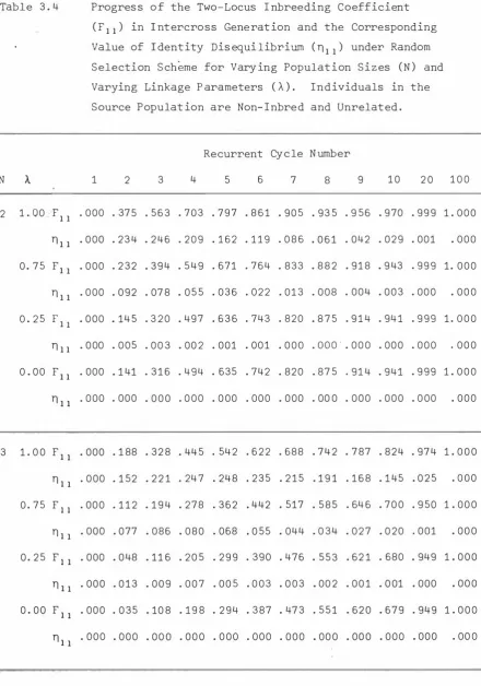
(39) 33 3. 5. Discus s i on Numerical res ults obtained by us ing the tran s it ion equat ions. ( 3 . 4 . 2 7 ) , ( 3 . 4 . 2 8 ) are shown in Tables 3 . 4 , 3 . 5 and 3 . 6 .. As men. t ioned above , th e initial generation is a s s umed to be non- inbre d and unrelated s o that for thes e initial individuals , prior to any s e lfing ,. 2. 1 + .A � 0 , 1 ) = [ 4 ' 1 , 1 , 1I 2 , 1 , 1 , 1 I 4 , 1 , 1I 4 , 1] and � 1 , 1 ) follows from equation ( 3 . 4 . 1 8 ) . As shown in the s e tab les , linkag e has a comp li cat ed effe ct on inbreeding at two loc i .. For comp lete l i nkag e , A = 1 , the equat ions. ( 3 . 4 . 27 ) , ( 3 . 4 . 2 8 ) do reduce correctly to the appropriate one-locus res ult s . When A = 0 , and the loci s egregate indep endent ly , CAI N and HINKE LMANN ( 1 9 7 0 ) claimed that the i nbreeding coefficient F 1 1 ( .A = O ) was the square o f the one- locus coeffi c i ent F 1 = F 1 1 ( .A= 1 ) . · Thi s is not the cas e here , or whenever there i s a cho ice of mat e s , and for genera l. A. an ident i ty dis equilibrium n 1 1 ( .A ) , mentioned on Page 2. was define d e arlier by WEIR and COCKERHAM ( 19 69b ) as. Values for the i dent ity dis equi librium are als o shown in Tab les 3 . 4 ,. 3 . 5 , and 3 . 6 .. The quant ity is pos it ive i n early generat ions , reaches. a maximum , and decreas es to zero with comp l e t e inbreed ing .. For comp letely. specifi ed pe digrees , however , such as afforded by the cas es of N = 2 or N = 3 , there i s no i dent ity disequilibr i um . I n genera l , in creased population s i ze i s seen t o delay the accrual of inbre e d ing , and t o a llow s e le ction t o be pra c t ised for a longer period . As N i ncreas es , the mi nimum and maximum i nbree d ing s chemes become more e xtreme .. As not ed above , the max imum i nbree d ing s cheme actually permits. inbre eding to in creas e with N .. The increas i n g divergen ce · in inbreed ing. levels between the minimum inbreeding s cheme and unres tri ct ed random s ele c t i on shows that the latter s cheme falls further behin d in e xploiting fully the advantages o f the intercross p has e i n this respect ..

(40) 34. A s CAIN and HINKELMANN ( 1 9 7 0 , 1 9 7 2 ) point out , t h e plant breeder is likely to be more con cerned with homozygos ity than with measures of i nbreeding .. An indivi dual i s homozygous when its homologous genes are. id e ntical by des cent or when they are identical in s t at e .. The former. i s the effect of i nbreeding and the probability of this o cc uring i s measured by the inbreeding coeffi ci ent .. The latter dep ends on the. chance of the union of genes having the same allel i c form .. Therefore. the inbreeding coeffi cients , F 1 , F 1 1 always provide lower bounds on the homozygos i ty at one and two loci resp ect ively . When ini tial gamet es are taken randomly from an infinitely large random mat i ng p opulation and indivi duals are reproduced by a pro cess without s elect ion , a knowledge of the population g ene frequencies , p . for allele a . , allows l l .. the expression of population genotyp i c frequencies in generation t as. p. P. a.. l. a.. l. (t). =. 2 p . + p . ( 1-p . ) F 1 ( t ) l l l. (t). =. [ 1 - F 1( t ) ] p . p . , i "I j 1 J. a.. 1. a. J. and the total amount of homozy gos ity as 1 - H(t). =. 1 - [ 1-F 1 ( t ) ] H ( O ). where H ( t ) is the amount of hetero zygos i ty in generation t .. Simi lar. expressions in the two- locus case can be found in COCKE RHAM and WEI R ( 197 3 ) .. When initial individuals are taken from a hetero zygous source ,. as i n recurrent select ion programmes , homozygosity can only b e caused by i dent i ty by des c ent and i denti ty in s tate of genes from different initial individuals .. The homozygos i ty i ndicated by the i nbreeding. measures is then likely t o b e c lose to total homozygosity .. A comp lete .. dis cus s i on of this problem requires the knowledge of the initial genotypi c frequencies and would need to take into a ccount the effects of th e s election programme on gene frequencie s ..

(41) 35 Tab l e 3 . 4. Progres s o f the Two- Locus I nbreeding Coefficient. ( F 1 1 ) in I nt ercro s s Gene rat ion and the Corresponding Value of I dent ity Dis equi libri um ( n 1 1 ) under Random S election S ch eme for Vary ing Populat i on S i z es ( N ) and Varying Linkage P arameters ( A ) .. I n d ividuals in the. S ource P opulat ion are Non- I nbre d and Unrelat ed .. Recurrent Cy c le N umber N. 2. 1. A.. 2. 3. 4. 5. 6. 7. 9. 8. 10. 20. 100. 1 .. 00 F 1 1 . 000 . 37 5 . 56 3 . 70 3 . 79 7 . 8 6 1 . 90 5 . 93 5 . 9 56 . 9 70 . 99 9 1 . 0 0 0 n 1 1 . 000 . 23 4 . 246 . 20 9 . 1 6 2 . 1 1 9 . 0 8 6 . 0 6 1 . 042 . 029 . 001. . 000. 0 . 7 5 F 1 1 . 000 . 2 32 . 39 4 . 5 4 9 . 671 . 764 . 833 . 8 8 2 . 91 8 . 9 43 . 99 9 1. 0 0 0 n 1 1 . 000 . 092 . 07 8 . 0 5 5 . 03 6 . 022 . 01 3 . 008 . 004 . 00 3 . 000 0 . 25. F1. . 00 0. 1 . 000 . 14 5 . 3 2 0 . 49 7 . 6 3 6 . 743 . 820 . 8 7 5 . 9 1 4 . 94 1 . 9 99 1 . 0 0 0. n 1 1 . 000 . 005 . 00 3 . 00 2 . 001 . 00 1 . 0 0 0. .. ooo. ·. . 00 0 . 000 . 000. . 00 0. 0 . 00 F 1 1 . 000 . 1 41 . 3 1 6 . 494 . 635 . 742 . 820 . 87 5 . 91 4 . 941 . 9 99 1 . 0 0 0 n 1 1 . 000 . 000 . 0 0 0 . 0 00 . 0 00 . 000 . 000 . 00 0 . 000 . 000 . 0 00 3. . 000. 1 . 0 0 F 1 1 . 000 . 1 88 . 32 8 . 44 5 . 54 2 . 6 22 . 688 . 74 2 . 7 87 . 824 . 97 4 1 . 0 0 0 n 1 1 . 000 . 1 52 . 2 2 1 . 24 7 . 248 . 23 5 . 2 1 5 . 1 9 1 . 1 6 8 . 1 45 . 0 2 5. . 0 00. 0 . 7 5 F 1 1 . 000 . 1 1 2 . 1 9 4 . 2 7 8 . 36 2 . 442 . 517 . 5 8 5 . 64 6 . 70 0 . 9 50 1 . 00 0 n 1 1 . 000 . 077 . 086 . 080 . 068 . 0 55 . 044 . 0 34 . 0 2 7 . 0 20 . 001. . 00 0. 0 . 2 5 F 1 1 . 000 . 048 . 11 6 . 20 5 . 29 9 . 390 . 476 . 5 5 3 . 62 1 . 680 . 949 1 . 0 0 0 n 1 1 . 000 . 0 13 . 00 9 . 00 7 . 00 5 . 0 0 3 . 0 0 3 . 00 2 . 00 1 . 0 01 . 000. . 00 0. 0 . 0 0 F 1 1 . 000 . 0 35 . 10 8 . 19 8 . 2 9 4 . 3 8 7 . 47 3 . 5 5 1 . 62 0 . 6 7 9 . 949 1 . 0 0 0 n 1 1 . 000 . 000 . 00 0 . 00 0 . 0 00 . 000 . 000 . 00 0 . 00 0 . 000 . 000. . 00 0.

(42) 36 Table 3 . 4. ( cont inued ). Recurrent Cyc le Number N. 4. 1. >... 1 . 00 0 . 75 0. 25. F1 1. 1. 00. 0 . 25. 6. 7. 8. 9. 10. 20. 100. . 000 . 1 50 . 270 . 374 . 462 . 5 3 9 . 604 . 660 . 7 0 8 . 7 50 . 946 1. 000 . 000 . 09 0 . 1 56 . 22 2 . 289 . 3 5 5 . 420 . 48 1 . 5 3 9 . 59 2 . 897 1 . 000. n1 1 F1 1. F1 1. . 0 0 0 . 0 6 7 . 083 . 083 . 0 7 5 . 06 5 . 0 55 . 046 . 038 . 0 31 . 002. . 000. . 000. . 0 0 0 . 0 3 8 . 086 . 1 5 1 . 223 . 297 . 37 0 . 440 . 5 0 5 . 5 6 5 . 89 5 1 . 000 . 000 . 016 . 014 . 01 1 . 009 . 00 7 . 006 . 00 4 . 00 3 . 003 . 000. . 000. . 000 . 028 . 077 . 1 43 . 2 1 6 . 29 2 . 366 . 4 3 7 . 50 3 . 5 6 3 . 894 1 . 000 . 000 . 006 . 004 . 00 3 . 003 . 00 2 . 00 2 . 00 1 . 0 0 1 . 0 0 1 . 000. . 000. . 00 0 . 068 . 1 30 . 1 88 . 242 . 2 9 3 . 340 . 384 . 42 5 . 46 3 . 7 30. . 9 99. . 000 . 064 . 11 3 . 1 5 3 . 1 84 . 207 . 224 . 2 37 . 244 . 24 9 . 19 7. . 001. . 00 0 . 041 . 070 . 09 6 . 1 22 . 1 48 . 17 5 . 20 3 . 2 3 2 . 26 2 . 5 5 1. . 99 8. . 0 00 . 036 . 0 5 3 . 0 6 1 . 0 6 3 . 0 6 2 . 06 0 . 05 6 . 0 5 2 . 04 7 . 01 8. . 00 0. . 00 0 . 0 1 7 . 031 . 049 . 0 7 1 . 0 97 . 1 2 6 . 1 5 6 . 1 8 9 . 22 2 . 536. . 99 8. . 0 00 . 01 3 . 014 . 014 . 0 1 3 . 0 1 2 . 010 . 00 9 . 00 8 . 00 7 . 00 2. . 000. F1 1. . 000 . 013 . 0 25 . 04 3 . 0 66 . 09 2 . 1 21 . 1 5 2 . 18 5 . 21 8 . 5 3 5. . 998. n11. . 000 . 0 0 8 . 009 . 00 8 . 00 7 . 006 . 0 0 6 . 00 5 . 0 0 5 . 00 4 . 001. . 000. F1 1. F1 1 n1 1 F1 1 n1 1. 0 . 00. 5. F1 1. n11. 0. 75. 4. . 00 0 . 1 28 . 197 . 2 34 . 249 . 249 . 239 . 2 24 . 2 0 7 . 1 8 8 . 051. n1 1. 10. 3. nl l. n1 1. 0 . 00. 2.

(43) 37 Table 3 . 4. ( cont inue d ). Recurrent Cyc le N umb er. 1. N. 25. 1 . 00. 0. 75 0. 25 0. 00. F11 n11 F1 1. n11 Fll n1 1 F1 1 n1 1. 1 0 0 1 . 00. F. 11. n1 1. 0. 75. F1. 1. n1 1. 0 . 25. F1 1 n1 1. 0 . 00. F1 1 nl l. 2. 3. 4. 5. 6. 7. 8. 9. 10. 20. 100. . 0 0 0 . 029 . 0 5 7 . 084 . 1 10 . 13 5 . 1 60 . 1 84 . 207 . 230 . 42 4 . 94 3 . 000 . 02 8 . 0 53 . 07 7 . 09 8 . 11 7 . 1 34 . 1 5 0 . 1 64 . 1 7 7 . 244 . 0 54 . 000 . 0 1 7 . 0 2 9 . 0 39 . 047 . 0 5 5 . 063 . 071 . 079 . 0 88 . 2 0 3 . 8 9 0 . 000 . 016 . 0 2 6 . 0 3 2 . 035 . 0 37 . 0 37 . 0 3 7 . 03 6 . 0 3 5 . 0 2 3 . 000 . 000 . 007 . 00 1 . 01 5 . 020 . 026 . 033 . 041 . 0 50 . 0 5 9 . 1 83 . 890 . 000 . 007 . 008 . 008 . 008 . 008 . 008 . 007 . 007 . 007 . 00 4 . 00 0 . 0 00 . 00 5 . 00 9 . 0 1 2 . 0 1 7 . 023 . 030 . 0 3 8 . 047 . 0 57 . 1 8 2 . 8 9 0 . 000 . 00 5 . 00 5 . 00 5 . 00 5 . 005 . 00 5 . 004 . 004 . 0 04 . 002 . 000 . 000 . 007 . 01 5 . 02 2 . 029 . 037 . 044 . 0 51 . 0 58 . 06 5 . 1 32 . 52 1 . 000 . 00 7 . 0 1 5 . 02 2 . 0 2 9 . 03 5 . 042 . 04 8 . 0 54 . 061 . 1 1 4 . 2 50 . 00 0 . 0 04 . 0 0 8 . 0 1 0 . 011 . 01 3 . 01 4 . 01 5 . 0 1 6 . 01 7 . 0 29 . 27 5 . 00 0 . 0 04 . 00 7 . 009 . 011 . 011 . 012 . 01 2 . 0 12 . 01 2 . 011 . 0 04 . 000 . 00 2 . 00 3 . 00 3 . 004 . 004 . 00 5 . 00 5 . 006 . 00 7 . 0 2 0 . 272 . 000 . 002 . 0 0 2 . 003 . 003 . 003 . 003 . 0 0 3 . 003 . 00 3 . 0 0 2 . 001 . 000 . 00 1 . 0 0 2 . 00 2 . 003 . 00 3 . 004 . 004 . 00 5 . 0 06 . 019 . 27 2 . 0 00 . 00 1 . 0 0 2 . 00 2 . 00 2 . 002 . 00 2 . 00 2 . 00 2 . 00 2 . 00 1 . 00 0.

(44) 38 Table 3 . 5. P rogress o f the Two- Locus I nbreeding Coeffic ient ( F 1 1 ) i n I ntercross Generat ion and the Corresponding Value of I dent ity Dis equil ibrium ( n 1 1 ) under Min imum I nbreed ing S e lect ion S cheme for Varying Populati on S i zes ( N ) and Varying Linkage P arameters ( A ) .. I ndivi duals in the. Source Popula t i on are Non-Inbred and Unrelat e d .. Recurrent Cycle Number. 1. N. 4. 1. 00. F1 1 n1 1. 0. 75. 0. 25. 0 . 00. F1 1 n1 1 F1 1 n11 F1 1 n1 1. 10. 1. 0 0 0. 75. F1 1 n1 1 F1 1 n1. 0 . 25. 0 . 00. 1. F1 1 n11 F1 1 nll. 2. 3. 4. 5. 6. 1. 8. 9. 10. 20. 100. . 0 0 0 . 1 25 . 2 2 9 . 3 2 1 . 402 . 474 . 536 . 59 2 . 641 . 68 3 . 91 2 1 . 0 0 0 . 0 00 . 109 . 1 7 7 . 2 18 . 240 . 249 . 249 . 242 . 23 0 . 21 6 . 0 81. . 00 0. . 0 0 0 . 07 5 . 1 2 8 . 1 8 0 . 234 . 2 89 . 344 . 39 8 . 4 51 . 5 0 1 . 83 5 1 . 0 0 0 . 00 0 . 0 59 . 07 6 . 0 7 7 . 0 7 2 . 0 6 5 . 0 56 . 04 8 . 0 4 1 . 0 34 . 00 5 . 000 . 032 . 0 6 7 . 1 1 5 . 1 71 . 232 . 294 . 3 5 5 . 414 . 47 0 . 83 1 . 00 0 . 016 . 01 4 . 01 2 . 00 9 . 007 . 006 . 00 5 . 004 . 00 3 . 00 0 . 0 0 0 . 0 2 3 . 0 5 9 . 1 0 8 . 1 66 . 227 . 290 . 3 52 . 41 2 . 46 8 . 8 30. . 000 1.. 0 00. . 000 1.. 000. . 00 0 . 008 . 00 6 . 00 5 . 0 04 . 003 . 002 . 002 . 0 01 . 00 1 . 000. . 000. . 000 . 042 . 081 . 1 19 . 1 5 5 . 19 0 . 2 23 . 2 5 5 . 286 . 3 1 5 . 5 5 0. . 984. . 0 0 0 . 040 . 07 5 . 10 5 . 1 31 . 1 54 . 173 . 19 0 . 2 04 . 21 6 . 248. . 01 6. . 00 0 . 02 5 . 042 . 0 56 . 06 9 . 082 . 095 . 10 9 . 1 24 . 1 39 . 323. . 969. . 00 0 . 023 . 0 36 . 042 . 045 . 04 6 . 045 . 044 . 0 42 . 040 . 02 1. . 0 00. . 0 0 0 . 0 1 1 . 0 1 1 . 024 . 034 . 0 45 . 0 58 . 073 . 088 . 10 6 . 3 0 5. . 969. . 00 0 . 0 0 9 . 01 0 . 01 0 . 010 . 0 09 . 008 . 0 08 . 0 0 7 . 00 6 . 003. . 0 00. . 0 0 0 . 00 8 . 0 1 3 . 02 0 . 030 . 041 . 05 5 . 0 6 9 . 0 86 . 10 3 . 304. . 969. . 000 . 006 . 00 7 . 006 . 006 . 00 5 . 00 5 . 00 5 . 00 4 . 00 4 . 002. . 000.

(45) 39 Table 3 . 5. ( cont inued ). Recurrent Cycle Number. 1. N. 25. 2. 3. ij. 5. 6. 7. 8. 9. 10. 20. 100. 1 . 0 0 F 1 1 . 0 0 0 . 016 . 031 . 046 . 0 61 . 07 5 . 09 0 . 104 . 11 8 . 1 3 2 . 2 5 8 . 7 88 n1. 1 . 0 0 0 . 0 1 5 . 0 30 . 044 . 0 57 . 07 0 . 0 8 2 . 09 3 . 1 04 . 1 1 4 . 19 1 . 16 7. n1. 1 . 0 0 0 . 009 . 0 1 5 . 01 8 . 0 21 . 02 2 . 023 . 023 . 0 2 3 . 02 2 . 01 8 . 002. 0 . 75 F 1 1 . 000 . 009 . 01 6 . 0 2 1 . 0 24 . 0 28 . 031 . 0 34 . 037 . 040 . 0 84 . 62 3 0 . 2 5 F 1 1 . 00 0 . 004 . 006 . 007 . 0 09 . 01 1 . 01 3 . 01 5 . 0 1 8 . 02 2 . 06 9 . 621 n 1 1 . 00 0 . 00 4 . 0 0 5 . 00 5 . 00 5 . 00 5 . 0 05 . 00 5 . 004 . 00 4 . 003 . 00 0. 0 . 00 F 1 1 . 00 0 . 003 . 0 04 . 0 0 5 . 007 . 0 09 . 01 1 . 0 1 4 . 0 1 7 . 0 20 . 068 . 62 1 n1. 100. 1.. 1 . 00 0 . 00 3 . 003 . 00 3 . 003 . 0 03 . 003 . 003 . 0 03 . 00 3 . 00 2 . 000. 00 F 1 1 . 00 0 . 00 4 . 0 08 . 011 . 015 . 019 . 0 2 3 . 0 26 . 030 . 0 34 . 07 0 . 31 3 n1. 1 . 00 0 . 004 . 008 . 011 . 01 5 . 01 8 . 0 2 2 . 0 26 . 02 9 . 0 32 . 06 5 . 21 5. 0 . 7 5 F 1 1 . 0 00 . 00 2 . 004 . 0 0 5 . 006 . 006 . 0 07 . 007 . 007 . 008 . 0 1 1 . 10 1 nll. . 0 00 . 00 2 . 004 . 00 5 . 006 . 0 06 . 006 . 006 . 0 07 . 00 7 . 006 . 004. 0 . 2 5 F 1 1 . 0 00 . 001 . 001 . 0 0 2 . 002 . 00 2 . 00 2 . 00 2 . 00 2 . 00 3 . 0 0 6 . 09 9 n1. 1 . 000 . 0 01 . 001 . 0 01 . . 001 . 001 . . 0 0 1 . 0 0 1 . 0 0 1 . 001 . 0 01 . 0 0 1. 0 . 0 0 F 1 1 . 0 00 . 0 01 . 001 . 001 . 001 . 001 . 00 1 . 0 02 . 00 2 . 00 2 . 0 06 . 0 9 8 n1 1. . 00 0 . 001 . 001 . 001 . 001 . 001 . 00 1 . 001 . 001 . 00 1 . 00 1 . 000.

(46) 40 Table 3 . 6. Progress of the Two- Locus Inbreeding Coefficient ( F 1 1 ) in I ntercros s Generation and the Corresponding Value of I dent i ty Dis equi librium ( n 1 1 ) under Maximum I nbreeding Select ion S ch eme for Vary ing P opulat ion S izes ( N ) and Vary ing Linkage Parameters ( A ) .. I nd ividuals in the. Source Pop ulat ion are Non- I nbred and Unre lated .. Recurrent Cy c le Number. 1. N. 4. 1 . 00. Fl l n1 1. 0 . 75. 0 . 25. 0 . 00. 1 . 00 0 . 75 0. 25. 0 . 00. 3. 4. 5. 6. 7. 8. 9. 10. 20. 100. . 000 . 1 56 . 2 80 . 3 86 . 47 6 . 554 . 619 . 67 5 . 7 23 . 764 . 9 52 1 . 000 . 000 . 1 32 . 20 2 . 2 3 7 . 249 . 247 . 236 . 2 1 9 . 2 00 . 1 80 . 046. . 000. F1 1. . 000 . 093 . 1 63 . 2 33 . 3 0 2 . 3 7 1 . 4 38 . 501 . 5 5 9 . 61 3 . 90 9 1 . 0 0 0. il l 1. . 000 . 0 69 . 08 5 . 0 84 . 0 75 . 0 65 . 054 . 0 4 5 . 036 . 0 29 . 00 3. F1 1. . 000 . 04 0 . 09 2 . 16 0 . 2 36 . 31 3 . 389 . 460 . 526 . 5 86 . 90 7 1 . 0 0 0. n11 F1 1 nn. 10. 2. F1 1 nll F1 1 nl i F1 1. . 0 00 . 01 5 . 0 1 3 . 0 1 1 . 0 09 . 007 . 0 0 5 . 004 . 0 03 . 00 3 . 000 . 000 . 029 . 082 . 1 5 2. · .. . 000. . 000. 229 . 308 . 385 . 4 5 7 . 524 . 584 . 906 1 . 0 0 0. . 000 . 00 5 . 004 . 0 0 3 . 00 2 . 002 . 001 . 00 1 . 001 . 001 . 000. . 0 00. . 000 . 1 58 . 28 3 . 390 . 481 . 558 . 6 24 . 68 0 . 7 2 8 . 7 69 . 9 54 1. 0 0 0 . 000 . 1 33 . 203 . 2 3 8 . 25 0 . 247 . 23 5 . 21 8 . 19 8 . 1 7 8 . 044. . 000. . 000 . 09 5 . 1 6 9 . 242 . 31 4 . 3 84 . 4 5 1 . 51 3 . 5 7 1 . 624 . 91 3 1 . 0 0 0 . 000 . 069 . 089 . 09 0 . 08 3 . 07 2 . 0 61 . 0 5 1 . 041 . 033 . 00 3. . 000. . 000 . 040 . 096 . 16 6 . 24 3 . 3 21 . 39 7 . 469 . 5 3 5 . 5 9 4 . 910 1. 0 0 0. n1 1. . 000 . 015 . 01 5 . 01 4 . 0 1 2 . 01 0 . 008 . 006 . 005 . 004 . 00 0. F1 1. . 0 00 . 03 0 . 08 5 . 1 56 . 2 34 . 31 4 . 39 2 . 464 . 5 3 1 . 5 92 . 91 0 1 . 000. n1 1. . 000 . 00 5 . 004 . 004 . 00 3 . 0 0 2 . 0 0 2 . 00 2 . 0 0 1 . 001 . 000. . 00 0. . 0 00.

(47) 41 Table 3 . 6. ( cont inued ). Recurrent Cy cle Number. 1. N. 25. 1. 00. 0 . 75. F1 1 n11 F1 1 n1 1. 0. 25 0 . 00. F1 1. 1. 00 0 . 75. F1 1. F1 1. 0 . 00. 4. 5. 6. 7. 8. 9. 10. 20. F1 1 1. F1 1 n1 1 F1 1 n1. 1. 100. . 0 00 . 174 . 307 . 420 . 51 4 . 5 9 3 . 6 5 9 . 7 1 5 . 7 61 . 8 00 . 96 6 1 . 0 0 0 . 0 0 0 . 1 44 . 2 1 3 . 244 . 2 5 0 . 241 . 225 . 204 . 1 8 2 . 1 6 0 . 0 3 3. . 000. . 000 . 1 0 4 . 1 86 . 267 . 34 6 . 4 22 . 492 . 5 57 . 6 1 6 . 6 6 9 . 9 3 5 1 . 0 0 0 . 000 . 074 . 09 2 . 091 . 08 2 . 070 . 058 . 047 . 037 . 0 29 . 00 2. . 000. . 0 00 . 044 . 1 09 . 1 89 . 2 7 5 . 360 . 441 . 516 . 58 3 . 643 . 9 33 1. 000 . 00 0. . 0 00 . 033 . 097 . 17 8 . 2 6 6 . 3 5 3 . 4 36 . 51 1 . 580 . 640 . 933 1. 0 0 0 . 00 0 . 002 . 002 . 00 2 . 00 2 . 001 . 0 01 . 00 1 . 001 . 0 01 . 00 0. . 000. . 00 0 . 1 84 . 32 3 . 439 . 5 3 5 . 614 . 6 80 . 7 35 . 7 80 . 8 1 8 . 97 2 1 . 0 0 0. n 1 1 . 0 0 0 . 1 5 0 . 21 9 . 246 . 249 . 237 . 21 8 . 19 5 . 1 7 1 . 1 49 . 02 7. n1. 0 . 25. 3. n l l . 0 0 0 . 0 1 4 . 0 1 4 . 01 3 . 01 0 . 008 . 007 . 00 5 . 004 . 00 3 . 00 0. n1 1. 100. 2. . 000. . 0 0 0 . 11 0 . 19 7 . 28 3 . 366 . 445 . 5 1 6 . 584 . 643 . 69 6 . 947 1 . 0 0 0. . 00 0 . 0 7 6 . 09 3 . 09 1 . 0 8 0 . 0 6 7 . 0 5 5 . 044 . 0 34 . 0 2 7 . 00 2. . 00 0. . 00 0 . 047 . 1 1 7 . 204 . 295 . 3 8 5 . 4 6 9 . 545 . 61 2 . 671 . 94 5 1 . 00 0 . 00 0 . 01 3 . 0 1 3 . 0 1 1 . 0 0 9 . 0 0 7 . 00 6 . 004 . 003 . 003 . 00 1. . 00 0. . 00 0 . 03 5 . 10 5 . 19 3 . 2 86 . 3 7 8 . 463 . 541 . 609 . 66 9 . 94 5 1 . 000 . 00 0 . 00 1 . 001 . 001 . 001 . 0 0 0 . 00 0 . 000 . 000 . 00 0 . 0 0 0. . 000.

(48) 42 ONE- AND TWO-LO CUS INBREEDI NG IN POPULAT I ONS. 4. WITH OVE RLAPP I N G GENERATIONS I ntroduction. 4.1. I n this Chapter , a s tu dy o f the inbree ding levels in populati ons with overlapping generat ions is presented with a view to quanti fying the effects of age s tructure in altering the genet i c progress of populations .. Relative t o p opulations of the same s i z e with j ust one. age class , it is known that inb re eding and hen ce h omozygos i ty is delayed in p opulat ions w ith several age clas ses .. I t is also known that the. cont inued pres ence of indivi duals , generally females , over s everal y ears in breeding programmes can delay the spread of favourable genes . I n another d irect ion , human populat i ons do not have dis crete generat ions , and this should b e reflect ed in mode ls of thes e populat ions .. This. Chapt er offers s ome novel features and presents some new result s for models of populations w i th overlapping generations . Most previous work. has conc entrated on the evaluat ion of inbre eding. and varian ce effective numb ers .. Previous authors include MORAN ( 19 6 2 ) ,. K I MURA and CROW ( 19 6 3a ) , N E I ( 1 9 7 0 ) , NEI and I MAI ZUMI ( 1 9 6 6 ) , GIESEL ( 1 969 ) , TURNE R and YOUNG ( 19 6 9 ) , FELSENSTEIN ( 1 9 7 1 ) , CROW and KIMURA ( 1 9 7 2 ) and H I LL ( 1 9 7 2a , 1 9 7 2b ) .. Effect ive numbers offer a very con. venient one-parameter des cript ion of the mating structure of a popula tion .. As such they are often us ed as a basis for comparison of di fferent. populat ions .. I n populations other than i deali zed one s , however , effec. tive numb ers are defined as limiting values ( over time ) of rates o f increas e of inbreeding o r dri ft variance .. Most populat ions d o not. maint ain the s ame characteri s t i cs for such long time p er iods , and in breeding programmes int erest is likely t o be centered on ear ly genera tions .. For thi s reason the following study concent rates also on. inbreeding levels in early generations , as did that o f J OHNSON ( 1 9 7 7 ) , rat h er than solely on the limit ing values of rates of change of i nbreeding .. This s tudy differs from that of JOHNSON , h owever , i n. restricting att ention t o e xa ct inbreeding levels . Thi s work follows H I LL ( 1 9 7 2a , b ) in broadening the s cope of s ome previous enquiri es by cons ideri ng both monoecious and d i oe cious populations , and not res tri cting atten tion to Poisson family s i ze ..

(49) 43 The s t udy of di fferent game t i c s ampling plans points out another restri ction in the exclusive concentration on effe ctive n umbers . I t. has been shown ( KI MURA and CROW 1 9 6 3b , COCKERHAM 1 9 7 0 ) that pop ulati ons that avoid early inbreeding may have high final rates of inb reeding.. The ranking of pop ulations on t he bas is of such final. rat es may be opposite to a ranking on the bas is of early inbreeding . O ther matters s uch as the ass umpt ions of constant overall popu lation s i ze , stable age dis tributi on and age-sp ecific b irth and death rates follow from convent ional mode ls . The one ent ire ly new feature o f thi s work on overlapp ing gene rations is t he treatment of inbreeding at two loc i .. The treatment is. bas ed on the g eneral methodology of WEIR and COCKERHAM ( 19 69b ) .. In. the ab s ence of linkage disequilibrium and s elect ion , t he two- locus inbre eding coeffi cient evaluat ed here allows two- lo cus genotypic Under the s ame condi t ions , a s might hold. frequencies to be s tudi ed .. in control populat ions , it has recently be en shown ( W E I R and COCKERHAM 1 9 7 7 ) h ow th e two- locus inbre eding coe ffi ci ent is used in the predi ct ion of means and variances of quantitat i ve traits .. Simi lar work to that. presented here allows the evaluation of other two- locus parameters which can be used to predict l inkage dis equilibrium ( COCKERHAM and WEIR 1 9 7 7 ) .. 4.2 4.2.1. Monoecious Dip loids Mating S cheme In all y ears t the population consists of N indivi duals b elonging. to various age clas s e s .. There are N . indivi duals in the ith clas s , l. and n clas s es , so that n. L. i= 1 Age i s measured in years .. N. = N . l. Each year N. n ewborn are added to the popu 1 of lation , all N n-year- olds di e , whi le a random sample of N . -N . n l l+ 1 the i -year- o lds die ..

(50) 44. The mat ing s cheme is random union of gametes an d i s speci fied by two sets of parameters .. S ampling b etween age c lasses is accommodat ed. by .parameters p , where p i is the probabi lity that a random gamete i rece ived by the newborn individuals in any year c ame from the ith age class in the previous year . n l:. i=1. p. = 1 . l.. For within age clas s es s ampl ing , arb itrary distribut ions are allowed for the numbers of gametes from individual members of th e class . us ual approach is. The. to as s ume that th ese numbers , or family s i zes , are. independently Poisson distributed s ub j ect to the n umbers adding to the total gamet i c output from that clas s .. The set of N . gamet i c numbers l.. from the ith age clas s are then mult inomi ally dis tribut e d .. A n analysis. of the different - distribut ions will b e given in S e ct i ons 4 . 4 and 4 . 5 . At present it is assume d that the gametic numbers h ave the s ame distri but ion for every member o f an age class , s o that there is a n eed for the use of gametic sampling probab i l it ies ( WE I R an d COCKERHAM 1 9 6 9b ) 2 11 P ( i ) and P ( i ) . The se are the probab ilities that two gametes from age class i are from one or two indivi duals respective ly with in that age class , an d. I t i s common ( e . g . JOHNS ON 19 7 7 ) to restrict attention t o the case where any output gamet e from an age class is equally likely to h ave come from any individual within the age class .. In this nequal-chance" case ,. There is a need in two-locus models for trigametic an d quadrigametic sampling probab i lities in addit ion to these digametic probab i lities .. 4.2.2. One-Locus Case. The quantity to b e determined is th� average inbreeding coefficient F 1 ( t ) of members of age class 1 in year t .. This is the average of the.

(51) 45 probabilit ies o f identity by des cent o f pairs o f genes drawn from indivi duals in the pre vious year , and each member o f a pair has probab i li ty p . of coming from an i-year - old , so that l.. n. l:. n l:. i=1 j = 1. P · P J· t h . ( t ) l. J l.. (4.2 . 1). .. The gamet i c s et me as ure � 1 ( t ) is the probabi lity of identi ty by l. J des cent of a gene from age c lass i and a gene from age c las s j in •. •. year t , and it will be necessary to es tabl ish transit ion equat ions for these game t i c s e t measures . When two gamete s are from the s ame age clas s , there is a chan ce that they are both from one indivi dual in that clas s , an d gen es on the. gametes may b e copies of the same gene in that individual . I dent ity by de s cent is then assure d � and to k eep track of such cas es the average coancestry 8 1 I . ( t ) h as been defined in Sect ion 2 . 2 as the probab i l ity J. l. J of ident ity by de s cent of a gene from a random member I . o f age c las s i l.. and a gen e from a random member J . of age class j , both in year t . J measure is averaged over all I . and J . . l.. The. J. I f primes denote distinct individuals in the same age class then , 2 � l i i ( t + 1 ) = P ( i ) 6 1 I . I . ( t+ 1 ) + P l.. l.. 11. C i ) 6 1 I . I ! ( t+ 1 ) , l.. l.. (4. 2. 2) ( 4 . 2 . 3). � l ij C t+ 1 ) = e 1 I . J . < t+ 1 ) , l. J. and there are the obvious symmetries e 1 r . J C t ) = e 1J . r . C t ) l. l. . J. J. Now an individual o f age i in year t + 1 was of age 1 in year t - i+ 2 ,. so gametes from s uch indi vi duals descended from parent s in year t - i + 1 . I dentity-by - des cent relations in equat ions ( 4 . 2 . 2 ) and ( 4 . 2 . 3 ) are. preserved if they are writ ten as.

No results found