Wavelet-based response spectrum compatible synthesis of accelerograms-Eurocode application (EC8)

City, University of London Institutional Repository

Citation

:

This is the unspecified version of the paper.

This version of the publication may differ from the final published

version.

Permanent repository link:

Link to published version

:

Copyright and reuse:

City Research Online aims to make research

outputs of City, University of London available to a wider audience.

Copyright and Moral Rights remain with the author(s) and/or copyright

holders. URLs from City Research Online may be freely distributed and

linked to.

Wavelets based response spectrum compatible synthesis of

accelerograms- Eurocode application (EC8)

Authors

A. Giaralis1, P.D. Spanos2*

Affiliations

1_{Ph.D. Candidate, Department of Civil Engineering, Rice University, Houston, Texas}

2 _{L. B. Ryon Chair in Engineering, Rice University, Houston, Texas}

Abstract

An integrated approach for addressing the problem of synthesizing artificial

seismic accelerograms compatible with a given displacement design/target spectrum is

presented in conjunction with aseismic design applications. Initially, a stochastic

dynamics solution is used to obtain a family of simulated non-stationary earthquake

records whose response spectrum is on the average in good agreement with the target

spectrum. The degree of the agreement depends significantly on the adoption of an

appropriate parametric evolutionary power spectral form which is related to the target

spectrum in an approximate manner. The performance of two commonly-used spectral

forms along with a newly proposed one is assessed with respect to the elastic

displacement design spectrum defined by the European code regulations (EC8).

* _{Pol D. Spanos, George R. Brown School of Engineering, L. B. Ryon Chair in}

Engineering, Rice University, MS 321, P.O. Box 1892, Houston, TX 77251, U.S.A.

Subsequently, the computational versatility of the family of harmonic wavelets is

employed to modify iteratively the simulated records to satisfy the compatibility criteria

for artificial accelerograms prescribed by EC8. In the process, baseline correction steps,

ordinarily taken to ensure that the obtained accelerograms are characterized by physically

meaningful velocity and displacement traces, are elucidated. Obviously, the presented

approach can be used not only in the case of the EC8, for which extensive numerical

results/ examples are included, but also for any code provisions mandated by regulatory

agencies. In any case, the presented numerical results can be quite useful in any aseismic

design process dominated by the EC8 specifications.

Keywords: Response Spectrum; Stochastic Processes; Accelerograms; Evolutionary

Power Spectrum; Harmonic Wavelets; Eurocode 8.

1. Introduction

Traditionally, code provisions for aseismic design of structures describe the

seismic severity by means of smooth design (response) elastic and inelastic spectra. This

practice facilitates significantly the design of regular structures in the framework of

equivalent linear static or dynamic analysis incorporating proper modal combination

rules. However, aseismic code regulations prescribe additional linear and/or non-linear

dynamic time-history analyses to be performed for the design of facilities of critical

importance and of structures incorporating non-conventional means of protection against

the seismic hazard (e.g. seismic isolation, energy dissipation devices, tuned-mass

recorded earthquake accelerograms associated with historical seismic events or by an

ensemble of numerically simulated earthquake signals. Typically, the response spectra of

the adopted time-histories must satisfy certain criteria of compatibility with the elastic

design spectra.

There are several factors likely to contribute to the extensive use of

time-integration analyses for the mitigation of the seismic hazard in the built environment in

the near future. These include the availability of more powerful computers, the increased

capabilities of commercial software to account for potential inelastic behavior of

structural systems, the need for constructing ever more sophisticated structured facilities

(e.g. base isolated structures, nuclear power plants e.t.c.), and for upgrading/retrofitting

the important/damaged existing ones. In this context, the development of dependable

tools to make readily available realistic design spectrum compatible seismic

accelerograms satisfying the related aseismic code provisions to practitioners is quite

pertinent.

Most of the early methods for the generation of response spectrum compatible

earthquake records are cited in the review articles of Ahmadi [1], and Spanos [2]. More

recent commonly-used methods for the purpose are described in the studies of Preumont

[3], Naeim and Lew [4], and Carballo and Cornell [5].

Lately, the problem at hand has been addressed by several researchers using

various non-traditional in the field of structural dynamics techniques. Wang et al. [6]

processed a collection of real accelerograms via the adaptive chirplet transform to reach a

joint time-frequency representation of the signals. Similarly, Wen and Gu [7] utilized the

an alternative time-frequency representation of individual accelerograms. In both of these

studies, the derived representations were used in conjunction with a common random

field simulation method to produce artificial seismic records possessing frequency

content and response spectra of similar characteristics to those attained by the original

recorded signals. Gupta and Joshi [8] and Shrinkhade and Gupta [9] cast the problem on a

purely stochastic basis by deriving response spectrum consistent power spectra. Then, the

phase characteristics of certain real accelerograms were used to introduce non-stationary

attributes in the generated artificial time-histories. Conte and Peng [10] obtained similar

results by considering a time-dependent (evolutionary) power spectrum numerically

estimated by individual real acceleration time-histories. Subsequently, non-stationary

artificial accelerograms compatible with this evolutionary power spectrum were produced

by way of a special adaptive least-square fitting scheme. Lin and Ghaboussi [11]

considered a relatively large ensemble of real accelerograms to “train” an appropriately

constructed stochastic neural network. Hence, the trained network was used to generate

artificial signals of comparable spectral and waveform characteristics with those of the

ensemble accelerograms given a design spectrum as input.

From a deterministic viewpoint, Karabalis et al. [12] incorporated certain

numerical schemes to appropriately modify individual recorded accelerograms so that

their response spectra are in close agreement with a given design spectrum. Mukherjee

and Gupta [13] and Hancock et al. [14] employed wavelet-based methods in the

frequency and in the time domain, respectively, for the same purpose. A considerably

different approach was proposed by Naeim et al. [15], incorporating a specific genetic

accelerograms out of a large databank obeying to certain design spectrum compatibility

criteria.

Obviously, in the preceding methods and in most of other ones proposed in the

literature, a suite of real seismic accelerograms is assumed to be available to the designer.

Ideally, it should include strong ground motion time histories recorded under certain soil

conditions and seismological environments related to the design spectrum with which

compatibility is ultimately pursued. Even though databases of recorded accelerograms are

being gradually extended, the formation of such a suite of signals may not be readily

feasible for specific seismically active regions. For instance, in some cases, such

databases contain incomplete background information about the provided signals.

Furthermore, the regulatory agencies may only provide a very “loose” classification of

soil types, while typically no detailed information is included about the seismogenetic

features of the source(s) considered in the definition of the design spectrum.

To circumvent the above requirement and the limitations of the deterministic

methods, a stochastic approach originally established in Spanos and Vargas Loli [16], is

followed in this paper to obtain ensembles of seismic records whose average response

spectrum bears close resemblance with a given design (response) spectrum. It should be

noted that this approach accounts for the non-stationarity of the generated signals in a

more direct manner than in the previous studies of Gupta and Joshi [8], and Shrinkhade

and Gupta [9]. In particular, a simulated earthquake accelerogram is construed as a

sample of a non-stationary zero-mean random process characterized by an analytically

defined uniformly modulated evolutionary power spectrum (EPS) [17]. The latter

maximum variance of the amplitude of the response of a single-degree-of-freedom

oscillator to a non-stationary stochastic excitation. An appropriate minimization problem

is formulated and solved numerically to determine the requisite parameters defining the

EPS. Upon determination of the EPS, an auto-regressive-moving-average model is

employed to simulate non-stationary artificial accelerograms compatible with the EPS

[18]. The obtained signals are then individually modified by means of the harmonic

wavelet transform [19, 20], in the context of an iterative scheme [13], to improve the

agreement of their response spectra with the target design spectrum. It is noted that the

unique attributes of the generalized harmonic wavelets provide enhanced flexibility in the

representation of signals throughout the frequency domain which enhances significantly

the efficiency of the original matching procedure of Mukherjee and Gupta [13]. In the

process, an efficient baseline correction technique is utilized [21] to yield accelerograms

possessing physically proper velocity and displacement traces.

The proposed methodology encompasses two distinct formulations: the stochastic

formulation where an appropriate EPS must be defined and the iterative matching

formulation whose efficiency depends on the construction of the harmonic wavelet basis

functions. Both of these formulations are extended and/or customized with respect to the

elastic displacement design spectrum, and the corresponding compatibility criteria for

artificial accelerograms set forth by the European aseismic code provisions (EC8) [22].

Nevertheless, adopting the specific code provisions does not limit the applicability of the

proposed methodology; it only exemplifies its versatility.

To this end, the potential of three different spectral forms of exponentially

EPS: the Kanai-Tajimi [23], the Clough-Penzien [24], and a novel one comprising a

predefined high-pass Butterworth filter (e.g. [25]) in series with the Kanai-Tajimi

spectrum. Furthermore, the construction of custom case-dependent harmonic wavelet

basis with scales of non-uniform width in the frequency domain is adopted to satisfy

efficiently the compatibility criteria mandated by the EC8.

2. Stochastic simulation of spectrum compatible artificial earthquake records

In this section, the pertinent theoretical background for associating an

evolutionary power spectrum with a given displacement response (design) spectrum is

first reviewed. Special attention is given to the analytical spectral form characterizing the

stationary part of this evolutionary power spectrum and alternative expressions are

considered for the purpose. A brief presentation of an efficient filtering method for

generating non-stationary signals being samples of an underlying evolutionary power

spectrum is also included.

2.1. Formulation of the simulation problem on a stochastic basis

Let the ground acceleration ug(t) due to a seismic event be modeled as a realization of a zero-mean separable non-stationary stochastic process expressed in the

domain of time t by the equation

( )

( ) ( )

g

u t =A t y t , (1)

evolutionary power spectrum S(t,ω) of the non-stationary process is expressed in the frequency (ω) domain as [17]

( )

( ) ( )

,

S t ω = A t S ω , (2)

where S(ω) is the two-sided power spectrum of the stationary process y(t).

Consider a unit-mass linear single-degree-of-freedom (SDOF) quiescent oscillator

with ratio of critical damping ζ and natural frequency ωn, base-excited by the process

ug(t). The motion of this system is governed by the equation

( )

( )

( )

( )

( )

( )

2

2

0 0 0

n n g

x t x t x t u t

x x

ζω ω

+ + = −

= =

, (3)

in which x(t) is the displacement trace of the oscillator relative to the motion of the ground and the dot over a symbol denotes differentiation with respect to time.

Assuming that the input energy, as expressed by S(t,ω), is distributed over a broad frequency band throughout the duration of the process ug(t), it can be argued that the response of lightly damped oscillators (ζ<<1) trails a pseudo-sinusoidal motion. That

is:

( )

( )

( )

x t =a t ⎡_⎣ω t+ϕ t ⎤_⎦, (4)

where α(t) and φ(t), are the response amplitude and phase and correspond to processes of slow temporal evolution statistics.

The aforementioned assumptions are common in the field of random vibrations

(see e.g. [26]), and reflect the fact that SDOF systems with small ratio of critical damping

attain highly resonant transfer functions centered at the natural frequency (ωn). Therefore,

these systems act as pass-band filters when excited by relatively broadband input, as is

dominated by the frequencies close to ωn. Under these assumptions, it can be shown that

the probability density function of the response amplitude follows a time-dependent

Rayleigh distribution [27]

( )

_{( )}

_{( )}

a a

a a

p a t

t t

σ σ

⎛ − ⎞

= ⎜_⎜ ⎟_⎟

⎝ ⎠, (5)

where the function σa2(t) is the variance of the amplitude given by the equation

( )

(

)

(

) (

)

2

2

0

exp 2 exp 2 ,

t

a n n n

n

t π t S d

σ ζω ζω τ τ ω τ

ω

= −

∫

To this end, a straightforward relation between a given (target) displacement

design spectrum Sd(ωn, ζ) and the evolutionary power spectrum of Eq. (2) can be established through the maximum value of the variance of the response amplitude [16]:

(

)

{

(

)

}

d n a n

S ω ζ =r σ ω ζ , (7)

where r is known as the “peak factor” [28]. In general, r depends on the stiffness (ωn),

and damping (ζ) of the SDOF oscillator, on the frequency content and duration of the

input process ug(t), and on the level of uncertainty furnished by the design spectrum as specified by regulatory agencies. The exact determination of the peak factor requires the

solution of the first-passage problem which is mathematically intractable, especially for

non-stationary input processes. It is pointed out that for stationary input processes some

reliable approximate formulae for estimating the peak factor exist in the literature (e.g.

[29], [30]). However, the use of such formulae for the determination of r in the case considered herein necessitates replacing the non-stationary process of Eq. (1) by an

equivalent stationary process of reduced duration [28]: an assumption which is not

non-stationary process. Therefore, for the purposes of the present study, r will be treated as a constant. Additional comments on selecting an appropriate value for the peak factor are

given in section 4 incorporating new numerical results pertaining to the EC8

displacement design spectrum [22].

2.2 Spectral form of the evolutionary power spectrum

In pursuing a solution to the simulation problem defined by Eq. (7), appropriate

analytical expressions for the modulation function A(t) and the power spectrum S(ω)

must be adopted. These must be compatible with the assumptions made in deriving Eqs.

(5) and (6) and should capture adequately the physical aspects of the problem.

In this regard, the Bogdanoff-Golberg-Bernard (BGB) envelope function defined

by [31]

( )

b A t =Ct ⎛_⎜− t⎞_⎟

⎝ ⎠ (8)

is used, where C>0 and 0<b<1 are parameters to be determined. This function accommodates appropriately the time-evolving intensity typically exhibited by recorded

seismic accelerograms; namely, a decaying segment preceded by a short initial period of

development. Note that the value of C is proportional to the peak ground acceleration, while the parameter b controls the shape of the envelope and thus the effective duration of the strong ground motion. Recently, the “slowly-varying” feature of the BGB function,

which must hold for Eq. (2) to be valid, was ascertained by means of the adaptive chirplet

( )

( )

ω ω ω ω

ω _ζ ω

ω ω ⎛ ⎞ + ⎜_⎜ ⎟_⎟ ⎝ ⎠ = ≤ ⎛ _{⎛ ⎞} ⎞ _{⎛ ⎞} ⎜ _{−⎜ ⎟} ⎟ _{+ ⎜ ⎟} ⎜ ⎟ ⎜ ⎟ ⎜ _{⎝ ⎠} ⎟ _{⎝ ⎠} ⎝ ⎠ , (9)

in which ωg and ζg are positive parameters and ωb signifies the highest frequency of

interest.

Setting G(ω)= 1 in Eq. (9) yields the well-known Kanai-Tajimi (KT) spectrum [23]. Apart from its simplicity, the main asset of the KT spectrum is that it lends itself to

a clear physical interpretation associated with site specific soil conditions. In particular, it

accounts for the resonant filtering effects that the surface soil deposits have on

propagating seismic waves by a linear SDOF system with natural frequency ωg and

damping ratio ζg. In this context, it has been extensively used in the past in random

vibration analysis of structures (e.g [28], [29]), and in strong ground motion

characterization (e.g. [33]). Nevertheless, the KT filter has the major disadvantage of

allowing for the presence of non-negligible low frequency content in the spectral

representation of the acceleration process ug(t). Such low frequency components are considerably accentuated upon integration of the accelerograms and have a significant

impact to their corresponding displacement traces. Specifically, this leads to displacement

time-histories exhibiting a monotonically increasing trend and yielding unrealistically

high permanent deformations similar to those reported in [4].

The Clough-Penzien (CP) spectral form incorporates a second order high-pass

filter to suppress the low frequency content allowed by the KT spectrum [24]. It is

( )

ω _ζ ω

ω ω ⎛ ⎞ ⎜ ⎟ ⎜ ⎟ ⎝ ⎠ = ⎛ _{⎛ ⎞} ⎞ _{⎛ ⎞} ⎜ _{−⎜ ⎟} ⎟ _{+ ⎜ ⎟} ⎜ ⎟ ⎜ ⎟ ⎜ _{⎝ ⎠} ⎟ _{⎝ ⎠} ⎝ ⎠ , (10)

in Eq. (9), where ωf and ζf are positive parameters related with the cut-off frequency and

the steepness of the transfer function of the high-pass filter G(ω). It is reasonable to attribute physical meaning to Eq. (10), since it coincides with the transfer function of a

SDOF system with natural frequency ωf and damping ratio ζf, and is used in series with

the KT filter. Indeed, some researchers have argued that ωf and ζf can be interpreted as

the stiffness and damping ratio of the geological formations of the crust of the Earth, the

bedrock (e.g. [34]). Nevertheless, the filter of Eq. (10) is primarily a signal processing

element, and thus, the values of parameters ωf and ζf should be set appropriately to

eliminate the spurious low frequencies [24]. In any case, note that by adopting the CP

spectral form the complexity of the simulation problem is significantly increased since

four more undetermined parameters are additionally introduced to the required

parameters, two, for the definition of the BGB modulating envelop. In this respect, it is

proposed to utilize a predefined standard infinite impulse response high-pass filter in

cascade with the KT band-pass filter. For instance, a Butterworth filter given by the

equation [25]

( )

N N

o

G ω ω

ω ω

=

+ (11)

can be assumed in Eq. (9), where N and ωο denote the filter order and cut-off frequency, respectively. These quantities can be judicially selected so that adequate filtering of the

of the simulation problem. Further elucidating comments on the various spectral forms

presented in this section are given in light of numerical results in section 4.1.

2.3 Approximate solution of the simulation problem

Combining Eqs. (2), (6), and (8) the following expression for the time-dependent

variance of the response amplitude is obtained

( )

{

( )

( )

( )

(

)

}

2 2 2

2 3 exp 2 exp 2exp 2exp 2

a n

n C

t π t bt t bt bt t

σ γ γ ζω

ω γ

= − − − + − − − , (12)

where

2 _n b

γ = ζω − . (13)

This expression possesses a global maximum at time t=t*. This time instant can be

determined by setting the first time derivative of Eq. (12) equal to zero. This criterion

leads to the condition

(

)

(

)

( )

2 ₂ * *2 _{2 1} * _{2 4 exp} * ₀ n

t bt bt b t

γ − − γ − − + ζω −γ = . (14)

Application of the previous operation in Eq. (6), and use of Eqs. (2) and (8) yields the

maximum value of the variance of the response amplitude. That is,

(

)

{

}

( )

( )

exp

max ,

2

a n n

n C t bt

S π

σ ω ζ ω

ζω −

= . (15)

An approximate solution to the simulation problem defined by Eqs. (7), (14), and

(15) is next pursued, as it has been proposed in [16]. In this regard, it is sought to satisfy

(

)

2 ₂

1

min M _{j j}

j S σ = ⎧ ⎫ − ⎨ ⎬

⎩

∑

where

( )

(

)

2 _{, , 1,...,}

0 , 1,..., 2

d n j j

S j M

S

j M M

ω ζ

⎧ ₌

⎪ = ⎨

= +

⎪⎩ , (17)

and

( )

( )

( )

(

)

(

)

( )

(

)

2 2 *2 *

3

2 * *2 *

*

exp

, 1,...,

2

2 2 1

2 4 exp , 1,..., 2

j j

n j n j

j j M j M j M j M j M j M j M n j M

r C t bt

S j M

t bt bt

b t j M M

ω ζω

σ γ γ

ζω γ − − − − − − − − ⎧ − ⎪ = ⎪ ⎪⎪ =_⎨ − − − − ⎪ − + − = + ⎪ ⎪ ⎪⎩ .. (18)

In Eqs. (16)-(18) the unknowns to be determined are the set of M time instants {tk*}, C, b, plus all necessary parameters involved in the analytical expression of S(ω), while the number of equations is 2M. In practice, the number of equations will always be greater than the total number of unknowns, since for an acceptable approximation to the

solution of the problem considered several tenths of points {ωn(j)} along the frequency band of concern should be included. Thus, Eqs. (16)-(18) define a typical

high-dimensional over-determined non-linear least-square fit optimization problem. In this

study, a Levenberg-Marquardt algorithm with line search is utilized to numerically solve

this problem (see e.g. [35]).

2.4 Generation of artificial non-stationary earthquake records

Upon solving the optimization problem of Eq. (16), the complete definition for

field simulation technique can be employed to synthesize an arbitrarily large number of

non-stationary accelerograms as realizations of the process characterized by S(t,ω). In the case of the uniformly modulated non-stationary stochastic processes, this task can be

carried out conveniently in two steps: First, stationary time histories y(t) compatible with a specific power spectrum S(ω) are generated. Next, the corresponding non-stationary time-histories are obtained by multiplying the stationary records with the envelop

function A(t), as Eq. (1) suggests. A plethora of techniques for synthesizing power spectrum compatible stationary signals exist in the literature. A self-contained exposition

of the topic presenting the most common of the methods is provided in [18].

In this study, the so-called ARMA simulation method is used. Specifically, a

discrete stationary stochastic process y is generated as the response of a linear time-invariant autoregressive moving average (ARMA) digital filter subject to clipped white

noise excitation [36]. The s-sample of an ARMA(p,q) process is calculated recursively as

a linear combination of the previous p samples plus a convolution term as follows

[ ]

[

]

[

]

1 0

p q

k l

k l

y s b y s k c w r l

= =

= −

∑

∑

, (19)

where the bk and cl are the coefficients of the ARMA filter. The symbol w denotes a discrete white noise process band-limited to ωb defined by the autocorrelation function

[ ] [ ]

{

}

E w u w v = ω δ . (20)

In this equation E{.} denotes the operator of mathematical expectation, and δuv is the Kronecker delta. Intuitively, the objective in this procedure is to “color” the latter process

via the ARMA filter so that the filtered process is characterized by the given power

and cl such that the squared modulus of the frequency response of the ARMA filter matches the power spectrum S(ω). Specifically, require that

( )

( )

s

i T

S ω = H eω . (21)

In Eq. (21) Ts is the sampling period of the discrete process which must comply with the Nyquist condition to avoid aliasing. That is,

s b T π

ω

≤ . (22)

Further, H denotes the transfer function of the ARMA filter which can be expressed as

( )

1 1 s s s q li T l i T l

p ki T k k c e H e b e ω ω ω − = − = = +

∑

∑

In the ensuing analysis the auto/cross-correlation matching (ACM) procedure is

used to determine the filter coefficients. In implementing this scheme, linear prediction

theory used in system identification is used to construct a relatively long autoregressive

(AR) digital filter to represent S(ω) as a first approximation. Next, the output auto-correlation and the input/output cross-auto-correlation sequences between this preliminary AR

and the final ARMA model are equated. Eventually, the coefficients of the ARMA filter

are calculated by solving a p+q by p+q system of linear equations. The mathematical

3. Enhanced response spectrum matching of synthesized records using the Harmonic Wavelet Transform

Obviously, the previously described procedure cannot guarantee that the response

spectrum of the individual synthetic signals produced will match exactly the target design

spectrum and satisfy the usual criteria for artificial accelerograms mandated by regulatory

agencies (see e.g. [22]). This is because of the various assumptions involved in the

formulation of the simulation problem, the approximate manner by which a solution to

this problem is sought, and the statistical nature characterizing the generation of the

signals by way of random field simulation.

Nevertheless, any arbitrary seismic accelerogram, whether artificial or recorded,

can be appropriately modified to improve the agreement of its response spectrum with the

target design spectrum. For this purpose, the generalized harmonic wavelets [19, 20] are

utilized herein for processing the generated accelerograms along with an iterative

matching procedure originally proposed in [13]. Compared to the modified

Littlewood-Pauley basis functions considered in [13], the generalized harmonic wavelets provide a

more flexible and balanced representation of signals throughout the frequency domain

[20]. Furthermore, advantage is taken of an efficient algorithm incorporating the Fast

Fourier Transform for the signal decomposition and reconstruction [37]. These attributes

render the Harmonic wavelet transform an effective tool for processing signals to achieve

enhanced response spectrum matching as will be shown in the ensuing numerical results.

This objective is achieved herein by an iterative numerical procedure combined with an

3.1 The Harmonic Wavelet Transform

Generalized harmonic wavelets have a box-shaped band-limited spectrum. A

wavelet of (m,n) scale and k position in time is represented in the frequency domain by the equation [19]

( ) (

)

(

)

n m n m

otherwise

ω _{ω ω ω}

ω ω

⎧ ⎛₋ ⎞

Δ ≤ ≤ Δ

⎪ ⎜_⎜ ⎟_⎟

Ψ =_⎨ − Δ _⎝ − _⎠

⎪ ⎩

, (24)

where m, n, and k are taken to be positive integer numbers in what follows and 2

o T

π ω

Δ = , (25)

with To being the total length of the time interval considered (i.e. the duration of the signals generated by Eq. (20)), in seconds. The time-domain Fourier Transform pair of

Eq. (25) is complex-valued [20], with magnitude

( )

(

)

(

)

( , ),

sin

o m n k

o

t k

n m

T n m

t

t k

n m

T n m

π ψ π ⎛ ⎛ ⎞ ⎞ − − ⎜ ⎜ ₋ ⎟ ⎟ ⎝ ⎠ ⎝ ⎠ = ⎛ ⎞ − − ⎜ ₋ ⎟ ⎝ ⎠ , (26) and phase

( )

(

)

( , ),m n k

o

t k

t m n

T n m

ϕ =π⎛_⎜ − ⎞_⎟ +

−

⎝ ⎠ . (27)

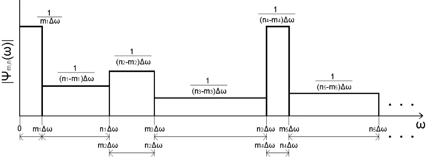
It has been proved [19] that a collection of harmonic wavelets spanning adjacent

non-overlapping intervals at different scales along the frequency axis, as shown

schematically in Fig. 1, forms a complete orthogonal basis. Then, the pertinent

(

)

( )

( )

o n m

W f m n k f t t dt T ψ ψ ∞ −∞ − ⎡ ⎤ =

⎣ ⎦

∫

projects any finite energy signal f(t) on this basis function. In Eq. (28) the bar over a symbol stands for complex conjugation. It is emphasized that the orthogonal property of

the harmonic wavelet basis allows for a perfect reconstruction of the original signal given

its HWT, and is associated with energy preservation concepts.

3.2 Iterative matching scheme

It can be deduced by the preceding exposition that the HWT decomposes a real

signal f(t) into several sub-signals fm,n (t), each one of them corresponding to a certain band of frequencies defined by the (m,n) pair, so that [20]

( )

( )

m n m n

f t =

∑

where

( )

(

)

( )

, ( , ),

0

2 Re n m , ,

m n m n k

k

f t − − W f_ψ m n k ψ t

=

⎧ _{⎡ ⎤} ⎫

= _{⎨ ⎣ ⎦ ⎬}

⎩

∑

Taking into consideration the discussions of section 2.1 concerning the shape of

the transfer function of lightly damped SDOF oscillators, it can be argued that a specific

part fmj,nj(t) of the original signal f(t) will mainly influence the response of those SDOF oscillators whose natural frequencies fall within the interval [mjΔω, njΔω]. Thus, an iterative modification procedure can be devised to improve the matching of the

( )

_{( )}

_{( )}

( )

_{( )}

v v m

m n m n n v m

S d

f t f t

D d ω ω ω ω ω ω ω ω Δ + Δ Δ Δ =

∫

∫

where D(v)(T) is the displacement response spectrum related to f(v)(t) which is obtained by Eq. (29). Note that a sufficient number of properly defined (m,n) pairs should be used to cover all frequencies of interest. Furthermore, the width (n-m)Δω of the various pairs can be arbitrarily small and varying among different scales, as illustrated in Fig. 1 for a given

duration To. This yields a significant advantage over the modified Littlewood-Pauley basis which defines intervals of logarithmically increasing width on the frequency

domain as it proceeds towards the higher frequencies [13]. Numerical evidence, and

additional comments on this feature of the harmonic wavelets in practical terms are

provided in sections 4.3 and 4.4.

3.3 Baseline correction considerations

Artificial seismic accelerograms to be used in the earthquake resistant design of

structures require that certain baseline corrections must be performed as in the case of

any recorded accelerogram [38]. This requirement has been reported and addressed by

several researchers in the past (e.g. [4], [12], [13]). It stems from the need to produce

accelerograms yielding realistic displacement traces. To this end, processing of the

accelerograms with a Butterworth high-pass filter of order 4 and cut-off frequency of

0.10Hz is employed in this study to acquire baseline corrected accelerograms.

Anti-causal zero-phase filtering is carried out. That is, the accelerogram is filtered once by the

and passes through the same filter again. In this manner, no phase distortion takes place,

and thus the properties of the filter considered have minimum impact on both the shape

of the displacement time-histories and the long period displacement spectral ordinates

[39]. Appropriate zero-padding before the initiation and at the end of the accelerograms is

performed before applying the anti-causal filter [40]. These pads are retained throughout

the integrations to construct compatible suites of acceleration, velocity and displacement

records [41].

4. Application to the Eurocode 8 design spectrum

This section provides numerical results pertaining to the displacement design

spectrum prescribed by the European aseismic code provisions (EC8) given in Appendix

A. In this context, an estimate for the value of the peak factor which yields a better

matching of the average response spectra of simulated accelerograms with the target

spectrum is proposed. Furthermore, an assessment of the three spectral forms of section

2.2 is included. The performance of the harmonic wavelet-based iterative scheme is also

demonstrated using a single simulated signal. Lastly, it is shown how to take advantage

of the versatility of the generalized harmonic wavelet basis to satisfy the compatibility

criteria for artificial accelerograms mandated by the EC8.

4.1 Selection of the peak factor r

to the ratio of the maximum mean (μ) over the maximum standard deviation (σ) for

Rayleigh distribution. That is, [16]

{ }

{ }

max

max 2

a a

r μ π

σ

= = . (32)

However, extensive numerical experimentation (Monte Carlo simulations), not included

here for brevity, pertaining to the EC8 design spectrum has shown that adopting the

above value for r yield rather conservative results. In particular, the obtained response spectral ordinates of the simulated time-histories tend to be, on average, rather larger than

the target ones for all natural periods considered. Notably, a similar trend is witnessed in

the numerical results of the relevant research work by Spanos and Vargas Loli (1985)

[16] for the case of the Newmark-Blume-Kapur and the Housner design spectra. In this

respect, it is noted that the aforementioned numerical experiments have suggested that, at

least in the case of the EC8 spectrum, adopting a peak factor 25% larger than that of Eq.

(32) yields ensembles of artificial accelerograms whose average response spectra are

close to the corresponding design spectra while a desirable level of conservatism is

maintained. Thus, the latter value is the one adopted for r for all the ensuing numerical results included in this study.

4.2 Assessment of various evolutionary power spectral forms

Let the EC8 displacement design spectrum for soil conditions B, damping ratio ζ=

5%, and peak ground acceleration (PGA) equal to 36% the acceleration of the gravity (g) be the target spectrum (see also the Appendix A). The minimization problem set by Eq.

(16) is solved for the three spectral forms defined in section 2.2. Namely the KT

Butterworth filtered Kanai-Tajimi (BWKT) spectrum (Eqs. (9) and (11)), modulated by

the BGB envelop function (Eq. (8)) on an interval [Tmin, Tmax] of the axis of natural periods. The numerical values of the requisite parameters to defining the design spectrum

compatible evolutionary power spectral forms under consideration are given in Table 1.

It is noted that in the BWKT case, the cut-off frequency ωo of the high-pass filter

of Eq. (12) has been judicially selected to coincide with the “corner” period TD= 2sec (see Fig. (A1) of Appendix A), prior to the solution of Eqs. (16)-(18). Incidentally, the value

of TD is the same for all soil types [22], and thus the selected value for ωο is globally applicable. Should this specification change in future versions of the EC8, it is suggested

to always set the cut-off frequency of the Butterworth filter equal to the corner period TD; extensive numerical testing has found this to be an effective choice. Moreover, the order

of the Butterworth filter was set to N= 2, so that a meaningful comparison with the CP case to be possible.

It should be noted that for all soil conditions, the EC8 assumes that the maximum

displacement of oscillators of natural period greater than 10 sec is independent of the

stiffness of the oscillators, that is, it attains a constant value equal to the maximum

displacement of the ground (see also Fig. A1 of Appendix A). Thus, extending the

point-wise matching to periods beyond 10sec will not capture any additional physics to the

optimization problem at hand. Hence, it is logical to assume Tmax= 10 sec. In both the CP and BWKT cases of Table 1 excellent point-wise matching at 100 frequencies ωn has

been achieved on the interval [0.63, 314.16] (rad/sec) which is mapped onto the interval

greater than TD= 2sec (i.e. to frequencies lower than 3.14 rad/sec) results in an unacceptably poor matching. An example is shown in Fig. 2 for Tmax= 4sec. In fact, the optimization algorithm completely fails in the KT case for Tmax>TE (= 5 sec for soil B).

This is because the KT spectrum does not incorporate enough “degrees of freedom” to

effectively trace the given design spectrum in the region of relatively long periods. This

aspect is interwoven with the incapability of the KT filter to effectively suppress the low

frequencies as have been discussed to some extent in section 2.2. This disadvantage of

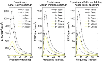
the KT spectral form can also be inferred by Fig. 3 where plots of certain evolutionary

power spectra of Table 1 are presented. In the same figure, it is observed that all spectra

remain relatively broad throughout their effective duration and that their energy becomes

negligible after 25 seconds.

Additional evolutionary CP power spectra compatible with EC8 design spectra for

two different levels of intensity, and for all soil types defined in EC8 are included in

Table 2. These results provide evidence that the values of the parameters yielded by the

optimization solver are not numerical artifacts but actually reflect the physical aspects of

the problem. Indeed, even though soil characterization is beyond the scope of the present

study, it can be readily seen that the various soil conditions are represented by the power

spectrum parameters. For instance, the value of ωg decreases while the damping ratio ζg

increases marching from stiff (i.e. type A) towards softer soil conditions (i.e. type D).

More importantly, Table 2 can be used as an interpolation guide for assigning initial/seed

values for the unknown parameters required by all common optimization algorithms for

the solution of Eqs. (16)-(18); this is especially pertinent in case the use of a different

Three ensembles of 40 accelerograms, each compatible with the KT (Tmax= 2sec), the BWKT, and the CP power spectra presented in Table 1 are synthesized using Eq. (19)

and a discrete version of Eq. (1). The sampling interval has been taken equal to 0.01 sec

to satisfy the condition of Eq. (22), and the duration of each record is 40sec. Baseline

corrected versions of these records have been also produced using the methodology

detailed in section 3.3. The average displacement response spectra for 5% damping of

each of the ensembles are plotted in Figs. 4-6 for both the uncorrected (dotted lines) and

the baseline corrected (solid lines) signals versus the target spectrum. In the same figures,

the largest and smallest maximum displacement responses along with the medians are

also shown versus the natural period of the oscillators considered to illustrate the

statistical nature of the obtained spectral ordinates.

The fact that the KT spectrum does not filter the very low-frequency content in

the acceleration traces causes difficulties in the corresponding displacement

time-histories. This attribute ultimately affects the matching of the displacement response

spectra with the target spectrum exhibiting undesirable trends as evidenced in Fig. (4).

Clearly, the KT spectrum is not an optimal choice for the purpose. However, both the

BWKT and the CP spectra yield satisfactory and practically similar results. Evidently,

these spectra can be used interchangeably to shape the form of the evolutionary power

spectrum of Eq. (2). To this end, note that the BWKT featuring the predefined high-pass

Butterworth filter involves fewer free parameters to be determined. Furthermore, it is

usually more convenient/ intuitive in practice to define a high-pass filter in signal

processing terms; namely by selecting the properties of a typical IIR filter, versus

proposed BWKT filter may be more advantageous over the CP filter from a practical

perspective.

4.3 Performance of the iterative Harmonic Wavelet-based matching procedure

In the context of the HWT, the efficiency of the iterative procedure outlined by

Eq. (31) to modify a certain accelerogram for achieving a better matching of its response

spectrum with a given design spectrum at all frequencies relies on the total number of the

wavelet scales (bins of Fig. 1) considered. For a specific range of frequencies, and

assuming uniform width for all scales, this number depends on the difference n-m (see Eq. (24)), and on the duration To of the accelerogram through the value of Δω (see Eq.

(25)). Addressing the second dependence, it is a common practice in standard Fourier

analysis to artificially augment the duration of a signal by adding zeros at the end of the

record for obtaining a more adequate representation of the original signal in the

frequency domain. This technique can be used herein to obtain a smaller value of Δω

which eventually yields a larger number of scales for a fixed value of n-m. Then, upon reconstructing the modified signal using Eq. (29), the artificially appended segment can

be discarded. It is noted that for all practical cases the latter operation will have negligible

impact on the response spectrum of the modified signal and thus on the matching with the

design spectrum, since most of the signal energy would have been released at earlier

times.

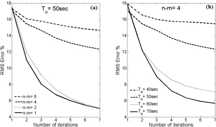
Fig. 7 provides a numerical example involving a single 40sec long artificial

accelerogram belonging to the previously presented BWKT ensemble to further elucidate

of the seismic record D(T) and the target spectrum Sd(T) is gauged against the number of iterations performed in terms of the root-mean-squared error (RMS). That is, the

( ) ( )

( )

2

1

1 Nk

d j j

j

k d j

S T D T

RMS error

N = S T

⎛ ₋ ⎞

⎜ ⎟

=

⎜ ⎟

⎝ ⎠

∑

is evaluated at Nk= 250 equally spaced points on the interval [0.02, 5] of natural periods

T. Note that evaluating the RMS error for T>5sec does not serve the purpose of assessing the performance of the iterative matching procedure since at this range of periods the

behavior of the response spectrum is primarily governed by the necessary baseline

adjustments (see also Figs. 4-6). In Fig. 7a four harmonic wavelet bases of various scale

widths (n-m), constant at all frequencies are used for processing the same artificially augmented record by 10sec of total duration To= 50sec. In Fig. 7b, the difference n-m is fixed to 2, and the original signal with To= 40sec plus three other records zero-padded to various total durations are considered. As expected, use of smaller n-m values and/or larger signal durations To achieves better and faster convergence of the response spectrum to the target spectrum. This, of course, comes at the expense of increased computational

effort per iteration.

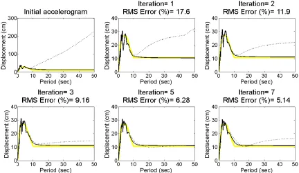
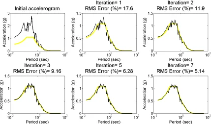
Figs. 8 and 9 provide snapshots of the improved matching achieved by means of

the proposed harmonic wavelet-based iterative scheme in terms of the displacement and

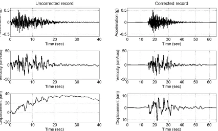
the pseudo-acceleration spectra respectively for n-m=2 and To= 50sec. Furthermore, Fig. 10 includes the acceleration, velocity and displacement time histories of the uncorrected

and the baseline corrected record considered in Figs. 8 and 9 after 7 iterations. The

obvious low-frequency unnatural trend of the displacement trace of the uncorrected

trace. As discussed in section 2.3, an appropriate number of zeros have been appended in

the beginning and at the end of the signal prior to the baseline adjustment [21]. These

padded segments are maintained throughout the integrations to derive a suite of

compatible acceleration, velocity, and displacement traces [40]. As can be inferred by

Fig. 10 ,this need is justified by the fact that both the velocity trace and to a greater extent

the displacement trace of the corrected accelerogram attain significant non-zero values

during these initial and final appended segments. These values are artifacts that represent

the end effects induced by the application of anti-causal filtering. However, their

relatively small intensity has minor contribution to the response spectral ordinates [39].

4.4 Adjustment of the Harmonic Wavelet basis to meet the EC8 compatibility criteria

Noticeably, most of the contemporary regulations adopt compatibility criteria for

artificial accelerograms to be used for the earthquake resistance design of structures

significantly different from what Eq. (33) suggests. For a structure of fundamental natural

period T1, the EC8 requires considering a collection of at least three accelerograms

obeying the following two rules: (a) The average of the zero period spectral response

acceleration values calculated from the individual time histories should be greater than

the product αgS (see also the Appendix), and (b) In the range of periods [0.2T1, 2T1] no

value of the average response spectrum for 5% damping, calculated from all time

histories, should be less than 90% of the corresponding value of the 5% damping design

spectrum [22]. These rules can be mathematically expressed by the equations:

1

1

1

s

N j j

s g

PGA N

a S

= _>

∑

and

( )

( )

min 0.90 , 0.2 2

s N j j s T d D T N

T T T S T

=

⎧ ⎫

⎪ ⎪

⎪ _{⎪ > ≤ ≤}

⎨ ⎬ ⎪ ⎪ ⎪ ⎪ ⎩ ⎭

∑

where Ns≥ 3 is the number of accelerograms considered while PGAj and Dj(T) are the peak ground acceleration and the displacement response spectrum of the j-th

accelerogram, respectively.

Taking advantage of the versatility of the generalized harmonic wavelets, already

discussed to some detail in section 3.2, a case-dependent wavelet base featuring scales of

non-uniform bandwidths (n-m)Δω across the frequency axis can readily be constructed. The objective is to have a more detailed discretization of the frequency domain in the

range of frequencies corresponding to the interval [0.2T1 2T1] and a sparser grid outside

this range. In this fashion, more weight is assigned to obtaining enhanced agreement of

the response spectral ordinates of the accelerograms with the target spectrum for the

oscillators whose natural frequencies lie closer to the fundamental period T1 of interest.

This renders the iterative matching procedure much more efficient and cheaper in

computational cost.

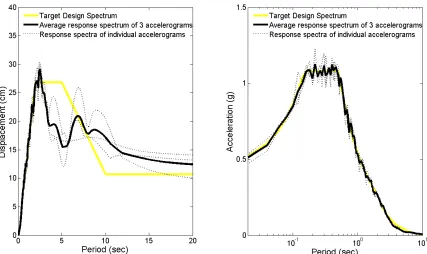
For instance, suppose a structure of fundamental natural period T1= 1.5 sec is to be designed for PGA= 0.36g and soil conditions B. Three arbitrarily selected

accelerograms out of the previously generated BWKT ensemble are processed using Eq.

(31) by means of a generalized harmonic wavelet basis with n-m =1 in the range of frequencies [2.09, 20.93] (rad/sec). This band corresponds to the range [0.3, 3] (sec) of

zero-padding at the end of the records has been considered prior to the modification of

the signals so that their total duration equals 50sec. This additional segment is completely

removed, as previously explained, after the required spectrum matching is achieved and

before any high-pass filtering for the baseline adjustment is made. After only four

iterations the compatibility criteria of EC8 are satisfied for the baseline corrected

artificial seismic signals. Specifically, the ratios of Eqs. (34) and (35) are computed as

1.19 (>1) and 0.92 (>0.90), respectively. The individual and the average displacement

and pseudo-acceleration response spectra of the three thus obtained signals are shown in

Fig. 11; Fig. 12 includes the acceleration, velocity and displacement traces these signals

in the time domain.

5. Concluding remarks

A stochastic approach for simulating non-stationary strong ground motion records

compatible with a given design displacement (target) spectrum in combination with a

harmonic wavelet-based iterative procedure have been presented. Without loss of

generality, the design spectrum prescribed by the European aseismic code provisions

(EC8) has been exclusively considered in all numerical examples provided.

At first, a previously established in the literature stochastic method has been

extended to relate in an approximate manner the target spectrum with a modulated

evolutionary power spectrum (EPS), which is parametrically expressed by an analytical

formula. This is accomplished by the use of a constant peak factor whose value has been

calibrated via Monte Carlo simulations pertaining to the EC8 design spectrum. Upon

spectrum have been synthesized using an appropriate auto-regressive-moving-average

filter driven by white noise. It has been shown numerically that a reasonable agreement

of the average response spectra of these accelerograms with the EC8 design spectrum can

be achieved if the assumed spectral form of the EPS can effectively suppress the spurious

low-frequency components of the underlying non-stationary process. In this respect, the

Kanai-Tajimi power spectrum has been found rather inappropriate for the purpose, while

the Clough-Penzien spectrum and a newly proposed Butterworth-filtered-Kanai-Tajimi

spectrum constitute viable choices for defining the requisite EPS.

It is acknowledged that the initially determined stochastic model yields

accelerograms whose frequency composition does not evolve with time, as is the case for

usual recorded seismic signals. Nevertheless, it does possess a significant practical merit

since it can yield any required number of design spectrum compatible artificial seismic

accelerograms, “from scratch”, without the need of having access to any real records.

Furthermore, it has been verified by numerically obtained EPSs associated with various

levels of seismic intensity and for all soil types prescribed by the EC8 that the proposed

approach captures reliably the site-specific soil conditions, as they are reflected in the

EC8 design spectrum. Clearly these results, given in a tabular form, can facilitate the

application of stochastic dynamics-based seismic risk assessment of contemporary

constructed facilities.

Subsequently, the wavelet transform has been employed to decompose the

simulated signals in a generalized harmonic wavelet basis of functions. In this regard, an

iterative scheme has been used to process individually each of the decomposed signals to

shown how to take advantage of the unique attributes of harmonic wavelets to construct

appropriately customized basis to efficiently treat small suites of simulated accelerograms

for satisfying compatibility criteria for artificial accelerograms posed by the EC8.

Special attention has also been given in obtaining records possessing realistic

velocity and displacement traces. In this respect, a state-of-the-art baseline correction

technique, used in the processing of recorded accelerograms pertaining to actual seismic

events, has been adopted. This step is critical for the design of extremely flexible

structures or of structures expected to exhibit severe inelastic behavior. In fact, the

attained values of the displacement spectral ordinates of the simulated records and thus

their closeness to the corresponding target spectrum in the region of long periods is

exclusively governed by the baseline adjustment considerations.

Obviously, the two distinct techniques presented in this study, namely the

evolutionary power spectrum-based representation of the seismic severity and the

subsequent wavelet-based iterative modification procedure of individual accelerograms

can be used independently to address, as well, certain needs arising in the practice of

aseismic design of structures. Specifically, the former may be used in conjunction with

any appropriate stochastic dynamics technique (e.g. Monte Carlo-based [18] or statistical

linearization-based [42]), for design scenarios necessitating the incorporation of the

uncertainty attributes of the seismic hazard, explicitly. Further, the latter can be readily

utilized to modify real recorded accelerograms in cases where accounting for the

temporal evolution of the frequency content of strong ground motions is deemed

essential. In both cases, the numerical results presented herein could be of particular

Acknowledgements

The financial support of this work by a grant from NSF is greatly acknowledged.

References

[1] Ahmadi G. Generation of artificial time histories compatible with given response spectra- A review. Solid Mech Arch 1979;4:207-239.

[2] Spanos PD. Digital synthesis of response-design spectrum compatible earthquake records for dynamic analyses. Shock Vib Digest 1983;15:21-30.

[3] Preumont A. The generation of spectrum compatible accelerograms for the design of nuclear power plants. Earthquake Eng Struct Dyn 1984;12:481-497.

[4] Naeim F, Lew M. On the use of design spectrum compatible time histories. Earthquake Spectra 1995;11:111-127.

[5] Carballo JE, Cornell CA. Probabilistic seismic demand analysis: Spectrum matching and design. Report RMS-41, Department of Civil and Environmental Engineering, Stanford University; 2000.

[6] Wang J, Fan L, Qian S, Zhou J. Simulations of non-stationary frequency content and its importance to seismic assessment of structures. Earthquake Eng Struct Dyn 2002;31:993-1005.

[7] Wen YK, Gu P. Description and simulation of nonstationary processes based on Hilbert spectra. J Eng Mech ASCE 2004;130:942-951.

[8] Gupta ID and Joshi RG. On synthesizing response spectrum compatible accelerograms. Eur Earthquake Eng 1993;7(2):3-12.

[9] Shrinkhande M and Gupta VK. On generating ensemble of design spectrum-compatible accelerograms. Eur Earthquake Eng 1996;10(3):49-56.

[10] Conte JP, Peng BF. Fully nonstationary analytical earthquake ground-motion model. J Eng Mech ASCE 1997;123:15-24.

[11] Lin C-CJ, Ghaboussi J. Generating multiple spectrum compatible accelerograms using stochastic neural networks. Earthquake Eng Struct Dyn 2001;30:1021-1042.

[13] Mukherjee S and Gupta VK. Wavelet-based generation of spectrum-compatible time-histories. Soil Dyn Earthquake Eng 2002;22:799-804.

[14] Hancock J, Watson-Lamprey J, Abrahamson NA, Bommer JJ, Markatis A, McCoy E, Mendis R. An improved method of matching response spectra of recorded earthquake ground motion using wavelets. J Earthquake Eng 2006;10:67-89.

[15] Naeim F, Alimoradi A, Pezeshk S. Selection and scaling of ground motion time histories for structural design using genetic algorithms. Earthquake Spectra 2004;20:413-426.

[16] Spanos PD, Vargas Loli LM. A statistical approach to generation of design spectrum compatible earthquake time histories. Soil Dyn Earthquake Eng 1985;4:2-8.

[17] Priestley MB. Evolutionary spectra and non-stationary processes. J Royal Stat Soc B 1965;27:204-237.

[18] Spanos PD, Zeldin BA. Monte Carlo treatment of random fields: A broad perspective. Appl Mech Rev 1998;51:219-237.

[19] Newland DE. Harmonic and musical wavelets. Proc Royal Soc Lond A 1994;444:605-620.

[20] Spanos PD, Tezcan J, Tratskas P. Stochastic processes evolutionary spectrum estimation via harmonic wavelets. Comp Meth Appl Mech Eng 2005;194:1367-1383.

[21] Converse AM, Brady AG. BAP: basic strong-motion accelerogram processing software, version 1.0. Open File Report 92-296A. United States Department of the interior Geological Survey; 1992.

[22] CEN. Eurocode 8: Design of Structures for Earthquake Resistance - Part 1: General Rules, Seismic Actions and Rules for Buildings. EN 1998-1: 2003 E. Comité Européen de Normalisation, Brussels, 2003.

[23] Kanai K. Semi-empirical formula for the seismic characteristics of the ground. University of Tokyo, Bull Earthquake Research Institute 1957;35:309-325.

[24] Clough RW, Penzien J. Dynamics of structures. Second Edition. Mc-Graw Hill, New York, 1993.

[25] Parks TW, Burrus CS. Digital Filter Design. John Wiley & Sons, New York, 1987.

[27] Spanos PD, Solomos GP. Markov approximation to transient vibration. J Eng Mech Div ASCE 1983;109:1134-1150.

[28] Vanmarcke EH. Structural response to earthquakes. Seismic Risk and Engineering Decisions (Eds. Lomnitz C, Rosenblueth E). Elsevier, Amsterdam, 1976.

[29] Der Kiureghian A. Structural response to stationary excitation. J Eng Mech Div ASCE 1980;106:1195-1213.

[30] Spanos PD. Numerics for common first-passage problem. J Eng Mech Div ASCE 1982;108:864-882.

[31] Bogdanoff JL, Goldberg JE, Bernard MC. Response of a simple structure to a random earthquake-type disturbance. Bull Seism Soc Am 1961;51:293-310.

[32] Politis NP, Giaralis A, Spanos PD. Joint time-frequency representation of simulated earthquake accelerograms via the adaptive chirplet transform. Computational Stochastic Mechanics-5 (Eds. Deodatis G, Spanos PD). Millpress, Rotterdam, 2007.

[33] Lai SP. Statistical characterization of strong ground motions using power spectral density function. Bull Seism Soc Am 1982;72:259-274.

[34] Manolis GD, Koliopoulos PK. Stochastic Structural Dynamics in Earthquake Engineering. WIT Press, Southampton, 2001.

[35] Nocedal J, Wright SJ. Numerical Optimization. Springer- Verlag, New York, 1999.

[36] Spanos PD, Mignolet MP. Z-transform modeling of p-m wave spectrum. J Eng Mech ASCE 1986;112:745-759.

[37] Newland DE. Time-frequency and time-scale signal analysis by harmonic wavelets. Signal analysis and prediction (Eds. Procházka A, Uhlír J, Rayner PJW, Kingsbury NG). Birkhaüser, Boston, 1998.

[38] Boore DM and Bommer JJ. Processing of strong-motion accelerograms: needs, options and consequences. Soil Dyn Earthquake Eng 2005;25:93-115.

[39] Boore DM, Akkar S. Effect of causal and acausal filters on elastic and inelastic response spectra. Earthquake Eng Struct Dyn 2003;32:1729-1748.

[40] Boore DM. On pads and filters: Processing strong-motion data. Bull Seism Soc Am 2005;95:745-750.

[42] Roberts JB, Spanos PD. Random Vibration and Statistical Linearization. Dover Publications, New York, 2003.

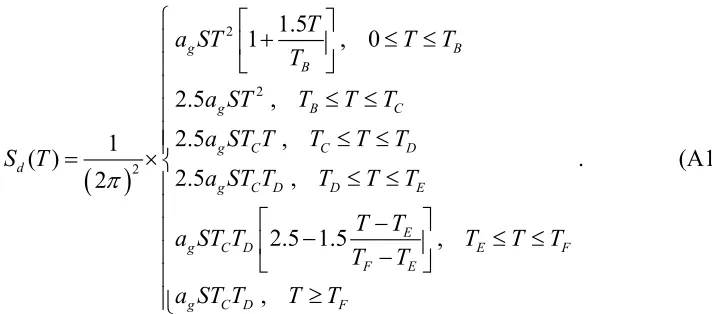
APPENDIX A

The elastic displacement response spectrum for oscillators with 5% ratio of

critical damping and natural period T, is defined by the European aseismic code

provisions (EC8) [22] by the expression

( )

2

2

2

1.5

1 , 0

2.5 , 2.5 , 1 ( ) 2.5 , 2

2.5 1.5 ,

,

g B

B

g B C

g C C D

d

g C D D E

E

g C D E F

F E

g C D F

T

a ST T T

T

a ST T T T a ST T T T T S T

a ST T T T T T T

a ST T T T T

T T a ST T T T

π ⎧ ⎡ ⎤ + ≤ ≤ ⎪ ⎢ ⎥ ⎣ ⎦ ⎪ ⎪ _{≤ ≤} ⎪ ⎪ ≤ ≤ ⎪ = _{× ⎨} ≤ ≤ ⎪ ⎪ _{⎡ − ⎤} ⎪ _{⎢ − ⎥ ≤ ≤} ⎪ _⎣ − _⎦ ⎪ ≥ ⎪⎩ . (A1)

In this equation, αg is the peak ground acceleration (PGA), S is a soil-dependent amplification factor, and TB, TC, TD, TE, and TF are soil-dependent corner periods which

define the various branches of the design spectrum, as shown in Figure A1. The values of

these quantities for the five different types of soil considered in EC8 are included in

Table 1. Parameters for the definition of various evolutionary power spectral forms compatible with the EC8 design spectrum for soil type B and peak ground acceleration

ag= 0.36g (g= 981 cm/sec2). KT spectrum

[Tmin= 0.02,Tmax= 2] (sec)

KT spectrum

[Tmin= 0.02,Tmax= 4] (sec)

BWKT spectrum

[Tmin= 0.02,Tmax= 10] (sec)

CP spectrum

[Tmin= 0.02,Tmax= 10] (sec) C= 19.05 cm/sec2.5

b= 0.51 sec-1

ζg= 0.71

ωg= 14.27 rad/sec

C= 7.66 cm/sec2.5 b= 0.25 sec-1

ζg= 0.47

ωg= 15.34 rad/sec

C= 17.20 cm/sec2.5 b= 0.45 sec-1

ζg= 0.74

ωg= 14.03 rad/sec

N= 2

ωο= 3.14 rad/sec

C= 18.29 cm/sec2.5 b= 0.46 sec-1

ζg= 0.78

ωg= 13.18 rad/sec

ζf= 0.88

ωf= 3.13 rad/sec

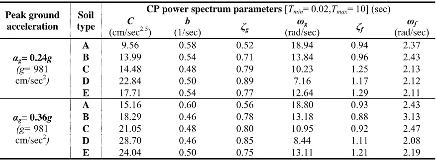
Table 2. Parameters for the definition of CP evolutionary power spectra compatible with various EC8 design spectra.

Peak ground acceleration

Soil type

CP power spectrum parameters [Tmin= 0.02,Tmax= 10] (sec)

C

(cm/sec2.5_{) (1/sec)} b ζg _(rad/sec) ωg ζf _(rad/sec) ωf

αg= 0.24g

(g= 981 cm/sec2₎

A 9.56 0.58 0.52 18.94 0.94 2.37 B 13.99 0.54 0.71 13.84 0.96 2.43 C 14.48 0.48 0.79 10.23 1.25 2.13 D 22.84 0.50 0.89 7.16 1.17 2.12 E 17.71 0.54 0.77 12.64 1.29 2.11

αg= 0.36g

(g= 981 cm/sec2₎

A 15.16 0.60 0.56 18.80 0.93 2.43 B 18.29 0.46 0.78 13.18 0.88 3.13 C 21.05 0.48 0.80 10.95 0.92 2.47 D 28.70 0.46 0.85 8.44 1.11 2.08 E 24.04 0.50 0.75 13.11 1.21 2.19

Table A1. Soil-dependent parameters for the definition of the EC8 design spectrum [22].

Soil type S TB (sec) TC (sec) TD (sec) TE (sec) TF (sec)

A 1.00 0.15 0.40 2.00 4.50 10.00

Fig. 1. An example of a generalized harmonic wavelets basis spanning non-overlapping intervals of arbitrary bandwidths in the frequency domain.

Fig. 3. Evolutionary power spectral forms given in Table 1. The plotted KT corresponds to the case of Tmax= 2sec.

Fig. 5. Displacement response spectra of an ensemble of 40 simulated accelerograms compatible with the BWKT evolutionary power spectrum given in Table 1.