Bandwidth selection for kernel density estimation with length-biased data

City, University of London Institutional Repository

Citation

:

This is the accepted version of the paper.

This version of the publication may differ from the final published

version.

Permanent repository link:

Link to published version

:

Copyright and reuse:

City Research Online aims to make research

outputs of City, University of London available to a wider audience.

Copyright and Moral Rights remain with the author(s) and/or copyright

holders. URLs from City Research Online may be freely distributed and

linked to.

City Research Online: http://openaccess.city.ac.uk/ [email protected]

Bandwidth selection for kernel density estimation with

length-biased data

M.I. Borrajo

, W. Gonz´

alez-Manteiga

and M.D. Mart´ınez-Miranda

a_{Departmento de Estat´ıstica, An´alise Matem´atica e Optimizaci´on,}

Universidade de Santiago de Compostela, Spain;

b_{Cass Business Shool, City University of London, 106 Buhill Row,}

EC1Y 8TZ London (UK)

Abstract

Length-biased data are a particular case of weighted data, which arise in many situations: biomedicine, quality control or epidemiology among others. In this paper we study the theoretical properties of kernel density estimation in the context of length-biased data, proposing two consistent bootstrap methods that we use for bandwidth selection. Apart from the bootstrap bandwidth selectors we suggest a rule-of-thumb. These bandwidth selection proposals are compared with a least-squares cross-validation method. A simulation study is accomplished to understand the behaviour of the procedures in finite samples.

Keywords: Bootstrap, Rule-of-thumb, Cross-validation, Non-parametric, Weighted data.

AMS Subject Classification: 62G07; 62G09; 62G20.

1

Introduction

Some specific examples are the visibility bias problem that arises when using aerial survey techniques to estimate, for instance, wildlife population density; or a damage model where an observation may be damaged by a process depending on the variable and then the observed data are clearly biased. Also the textile fibres problem is a classical motivating example.

Let us denote by f the density function of an unobserved random variable X, and sassume that the available information refers to a closely related random variable Y with weighted or biased distribution determined by the density function:

fY,ω(y) =

ω(y)f(y)

µω

y >0,

where ω is a known function and µω =

R

ω(x)f(x)dx <∞.

A particular case of weighted data is the length-biased data, where the probability of an observation to be sampled is directly proportional to its value in a simple linear way. In this case the weight function that determines the bias is the identity function, i.e.,

ω(y) =y. This sort of data are quite common in problems related to renewal processes, epidemiological cohort studies or screening programs for the study of chronic diseases, see Zelen and Feinleib (1969).

Cox (2005) proposed an estimator for the mean and another for the distribution func-tion in the context of weighted data. Vardi (1982, 1985) showed that this last estimator was the maximum likelihood estimator of the distribution function under weighted sam-pling and that the estimation of the mean is √n−consistent. Density estimation for this type of data started in the 80’s when Bhattacharyya and Richardson (1988) defined the first density estimator for length-biased data based on the problem of fibres, which was continued with theoretical developments in Richardson et al. (1991). Furthermore, Jones (1991) proposed a modification of the common kernel density estimator adapted to length-biased data which is widely used. In the same paper he showed that this proposal has some advantages over the previous one, and better asymptotic properties. Ahmad (1995) extended to the multivariate case these two kernel density estimators. Another extensions using Fourier series have been proposed in Jones and Karunamuni (1997). Later a third non-parametric estimator has been considered in Guillam´on et al. (1998).

Density estimation for weighted data has also been studied from other points of view, Barmi and Simonoff (2000) proposed a simple transformation-based approach motivated by the form of the non-parametric maximun likelihood estimator of the density. Efro-movich (2004) presented asymptotic results on sharp minimax density estimation. Pro-jection methods are developed in Brunel et al. (2009). Asgharian et al. (2002) and de U˜

na-´

The use of non-parametric methods implies to choose a bandwidth parameter, which determines the degree of smoothness to be considered in the estimation. The choice of the bandwidth parameter is crucial and it has motivated several papers in the literature in the recent decades. Marron (1988), Scott (1992) and Silverman (1986) provide a full description of the problem as well as a review of several bandwidth selection methods. Later methods such as plug-in or bootstrap methods, have been defined in Hall and Marron (1987), Sheather and Jones (1991) and Marron (1992). Fourier transforms have also been used in this context, see Chiu (1992). To explore the most relevant bandwidth selection methods in density estimation for complete data see the reviews of Turlach (1993), Cao et al. (1994), Jones et al. (1996) or Heidenreich et al. (2013), and the recent work on local linear density estimation by Mammen et al. (2011, 2014).

This paper is organised as follows. In Section 2 we develop asymptotic theory for the kernel density estimator of Jones (1991) for length-biased data, and we also define two different consistent bootstrap procedures. In Section 3 we propose new data-driven bandwidth selection methods: a rule-of-thumb based on the Normal distribution and two bootstrap bandwidth selectors based on the procedures presented in the previous section. These proposals are competitors of a cross-validation method which, to the extent of our knowledge, is the only existent data-driven bandwidth selector in this context. In Section 4, we carry out an extensive simulation study to evaluate the performance of the presented bandwidth selectors for finite samples. We draw some conclusions in Section 5. Final remarks are given in Section 6 as well as a discussion of how the methodology developed in this paper can be generalised to a widespread weight function. Finally we add in the appendix the proofs of the theoretical results.

2

Theoretical developments

Hereafter we will work under the scenario of the length-biased data even though all the results can be generalised to the weighted data case under appropriate assumptions, see final remarks in Section 6.

Hence, let us write the density function of the observed variable Y as

fY(y) =

yf(y)

µ , y >0,

with µ=R

yf(y)dy.

LetY1, . . . , Ynbe an i.i.d. (independent identically distributed) sample fromfY, Jones

(1991) defined the following kernel density estimator based on the structure of the one proposed in Parzen (1962) and Rosenblatt (1956):

ˆ

fh(y) =

1

nµˆ

n

X

i=1

1

Yi

Kh(y−Yi), (1)

In the following result we obtain the value of the pointwise mean and variance of ˆfh

with the corresponding error rates, as well as its mean squared error (MSE), which is defined as:

MSE(h, y) = Eh( ˆfh(y)−f(y))2

i

.

We need to introduce the following hypotheses: (A.1) E_X1 <+∞, E_Y12ν

<+∞ where ν ∈_N, ν ≥3, (A.2) R K(u)du= 1, R uK(u)du= 0 andµ2(K)<+∞,

(A.3) limn→∞nh= +∞,

(A.4) y a continuity point off,

(A.5) f has two continuous derivates,

(A.6) K is twice differentiable.

Theorem 2.1. Under conditions (A.1) to (A.4) we have:

E

h

ˆ

fh(y)

i

= (Kh◦f) (y) +O

1

n

and

V ar

h

ˆ

fh(y)

i

=n−1 K_h2◦γ(y)−(Kh◦f)

2

(y)+O

1

n

,

where ◦ denotes the convolution between two functions and γ(y) = µf(y)/y. Moreover, adding condition (A.5), we have:

MSE (h, y) = 1 4h

4_f00_(y)2_µ2 2(K) +

γ(y)

nh R(K) +o

h4+ 1

nh

, (2)

where µ2(K) = R

u2_{K(u)du and R(K) =}R

K2_(u)du.

Now, defining the mean integrated squared error (MISE) as

MISE(h) =E

Z

ˆ

fh(y)−f(y)

2

dy, (3)

and denoting by AMISE its asymptotic version, the following result is a consequence of Theorem 2.1.

Corollary 2.2. Under conditions (A.1), (A.2), (A.3) and (A.5),

MISE (h) = 1 4h

4

µ2₂(K)R(f00) + R(K)µc

nh +o

h4 + 1

nh

,

AMISE (h) = 1 4h

4_µ2

2(K)R(f

00

) + R(K)µc

nh , with c=

Z

1

yf(y)dy.

As a consequence, the optimal bandwidth value which minimises AMISE(h) is:

hAMISE =

R(K)µc nµ2

2(K)R(f

00

)

1/5

2.1

Resampling bootstrap methods

In this section we develop two different bootstrap procedures that can be applied in the context of length-biased data. Both of them are consistent in the way it is shown below and they conform the basis to define different data-driven bandwidth selection methods.

2.1.1 Bootstrapping using Jones’ estimator

In this first mehtod we follow the work by Cao (1990, 1993) using the so-called smooth bootstrap to develop a bandwidth selector for the kernel density estimator of Jones (1991), given in (1). It is remarkable that one bootstrap bandwidth selector can be implemented in practice without requiring resampling and any Monte Carlo approximation.

Given an i.i.d. sample, Y1, . . . , Yn from fY, and ˆfg the density estimator introduced

in (1) with pilot bandwidth g, the smooth bootstrap samples, Y₁∗, . . . , Y_n∗, are generated by sampling randomly with replacement n times from the estimated density ˆfY,g(y) =

yfˆg(y)/µˆ.

Let Y∗ denote the random variable generated by the bootstrap method presented above. From the bootstrap sample let define the bootstrap density estimator of Y∗ as

ˆ

f∗

h(y) =

1

nµˆ ∗

n

X

i=1

1

Y_i∗Lh(y−Y ∗

i ), (5)

where ˆµ∗ =

1

n

Pn

i=1

1

Y_i∗

−1

, andLh(·) = _h1L(_h·), withLbeing a symmetric kernel function

like K.

The following result provides the expression of the mean, the variance and the mean squared error of ˆf_h∗(y) under the bootstrap distribution. We use the notation E∗, V ar∗

and MSE∗ to refer to the bootstrap distribution.

Theorem 2.3. Under conditions (A.1) to (A.4)

E∗hfˆ∗

h(y)

i

=Lh◦fˆg

(y) +OP

1

n

and

V ar∗hfˆ∗

h(y)

i

=n−1

L2_h◦γˆg

(y)−Lh◦fˆg

2

(y)

+OP

1

n

.

Moreover, adding condition (A.6), we obtain

MSE∗(h, y) = 1 4h

4_ˆ

f_g00(y)

2

µ2₂(L) + γˆg(y)

nh R(L) +oP

h4+ 1

nh

,

where ˆγg(y) = ˆµfˆg(y)/y, µ2(L) = R

u2_{L(u)du and R(L) =}R

Corollary 2.4. Under hypothesis (A.2), (A.3), (A.4) and (A.6)

MISE∗(h) = 1 4h

4_µ2

2(L)R( ˆf

00

g) +

R(L)ˆµˆc nh +oP

h4+ 1

nh

,

AMISE∗(h) = 1 4h

4_µ2

2(L)R( ˆf

00

g) +

R(L)ˆµˆc

nh , with ˆc= ˆµ

1

n

n

X

i=1

1

Y2

i

.

Therefore, the asymptotic expression of the optimal bootstrap bandwidth is:

hAMISE∗ =

R(L)ˆµˆc nµ2

2(L)R( ˆf

00

g)

!1/5

,

which is a plug-in version of (4).

The following corollary is a consequence of the previous results.

Corollary 2.5. Under assumptions (A.1) to (A.4), MISE∗ and AMISE∗ are consistent estimators of MISE and AMISE, respectively.

2.1.2 Bootstrapping using a common kernel density estimator

In this second method, we are also using a smooth bootstrap procedure in which we will use a common kernel density estimator instead of Jones’. The idea of defining this second procedure is to be able to use the methodology developed in Bose and Dutta (2013) for bandwidth selection in kernel density estimation.

Given an i.i.d. sample, Y1, . . . , Yn from fY, and denote by ˜fK,g the common kernel

density estimator with pilot bandwidth g and a kernel function K, the smooth bootstrap samples,Y₁∗, . . . , Y_n∗, are generated by sampling randomly with replacementntimes from

˜

fK,g. Let Y∗ denote again the random variable generated by the bootstrap method

pre-sented above. From the bootstrap sample let us define the bootstrap density estimator of

Y∗ as the one presented in (5), taking into account that the bootstrap sample is generated differently.

Now we provide the expression for the point wise mean and variance of ˆf_h∗(y) under this bootstrap distribution.

Theorem 2.6. Under conditions (A.1) to (A.4)

E∗hfˆ_h∗(y)i = _R 1

1

zf˜K,g(z)dz

Z

1

zLh(y−z) ˜fK,g(z)dz+OP

1

n

and

V ar∗hfˆ∗

h(y)

i

= 1

nR 1_zf˜K,g(z)dz

2 Z ₁

z2L 2

h(y−z) ˜fK,g(z)dz−

Z ₁

zLh(y−z) ˜fK,g(z)dz

2

+

+OP

1

n

Moreover,

MSE∗(h, y) =

R ₁

zLh(y−z) ˜fK,g(z)dz

R ₁

zf˜K,g(z)dz

−fˆh(y)

!2

+

+ 1

nR 1_zf˜K,g(z)dz

2

Z ₁

z2L 2

h(y−z) ˜fK,g(z)dz −

Z ₁

zLh(y−z) ˜fK,g(z)dz

2

+

+OP

1

n

.

Remark that for this bootstrap method we do not get manageable explicit expressions of the error criteria as we got in the previous one; and the way to obtain MISE∗(h)is integrating the expression above, but we neither obtain an explicit expression.

3

Bandwidth selection

In this section we describe bandwidth selection methods for the density estimator defined in (1). These methods consist of adaptations of common automatic selectors for kernel density estimation with complete data to the context of length-biased data. We propose a Normal scale rule and two bootstrap selectors derived from the consistent resampling procedures given in the previous section. These proposals are defined as competitors of the cross-validation method proposed in Guillam´on et al. (1998).

Two new methods are based on estimating the infeasible optimal expression (4), in which the unknown elements are R(f00), c and µ. However, we have previously shown that these last two terms can be easily estimated, and then the only term that still needs to be estimated is R(f00). The last bootstrap bandwidth selection procedure is based on the minimisation of the M ISE∗(h) and does not require those estimations.

3.1

Rule-of-thumb for bandwidth selection

This method is based on the rule-of-thumb, Silverman (1986), for complete data. The idea is to assume that the underlying distribution is Normal, N(µ, σ), and in this situation

R(f00) = 3 8π

−1/2_σ−5_.

To get a suitable estimator of σ in the context of length-biased data is not trivial. We suggest to estimate it as follows. Cox (2005) states that EY [Xr] =

µr+1

µ , where µr+1

denotes the (r+1)-th order moment of the original and not observable variable X. So,

thus,

ˆ

σ2 = ˆµ2−µˆ2 =

1

n

n

X

i=1

1

Yi

!−1



1

n

n

X

i=1

Yi

!

− 1

n

n

X

i=1

1

Yi

!−1

,

and finally

ˆ

hRT =

R(K)ˆµˆc8√π nµ2

2(K)3 1/5

ˆ

σ.

Another possible estimator forσ could be obtained using a robust method such as the interquartile range (IQR)

ˆ

σIQR =

IQR

Φ−1_(0.75)−Φ−1_(0.25),

where Φ is the Normal distribution function.

3.2

Cross-validation

The method previously defined is based on minimising estimations of the MISE, more precisely of the AMISE. This procedure relies on the minimisation of the ISE (integrated squared error), the methodology is the same as in Rudemo (1982) and Bowman (1984) applied to (1), and it was developed in Guillam´on et al. (1998).

Let write:

ISE(h) =

Z

ˆ

fh(z)−f(z)

2

dz =

Z

ˆ

f_h2(z)dz−2

Z

ˆ

fh(z)f(z)dz+

Z

f2(z)dz. (6)

Note thatR f2(z)dz does not depend onh, so the minimisation of the ISE is equivalent to minimise the following function:

Z

ˆ

f_h2(z)dz−2

Z

ˆ

fh(z)f(z)dz =

Z

ˆ

f_h2(z)dz−2E[ ˆfh],

which can be estimated by

CV(h) =

Z

ˆ

f_h2(z)dz−2E[[ ˆfh].

The addends of this estimation may be expressed as follows:

Z

ˆ

f_h2(z)dz =

Z ₁

nhµˆ

n

X

i=1

1

Yi

K

z−Yi

h

!

1

nhµˆ

n

X

j=1

1

Yj

K

z−Yj

h

!

=n−2h−1µˆ2

n

X

i=1

n

X

j=1

1

Yi

1

Yj

(K◦K)

Yi−Yj

h

[

E[ ˆfh] = ˆµn−1 n

X

i=1

ˆ

f−i(Yi)

Yi

= ˆµn−1

n

X

i=1

Y_i−1 X

j6=i

1

Yj

!−1 X

j6=i

1

Yj

Kh(Yi−Yj)

!

,

realising thatE[ ˆfh] =

R _ˆ

fh(z)f(z)dz =

R _ˆ

fh(z)µfY_z(z)dz, and define ˆf−i as the estimator in

(1) calculated with all the data points except Yi.

The cross-validation bandwidth is obtained following the proposal in Dutta (2016), where the CV function is minimized in a compact interval of the form [c1IQRn−1/5, c2IQR(log(n)/n)1/5], where IQR is the inter-quartile range and c1 and c2

are positive constants (see Dutta (2016) for the choice of these values). We will be de-noted hereafter this bandwidth value as ˆhCV.

3.3

Bootstrap for bandwidth selection

3.3.1 Using Jones’ estimator

The asymptotic expression of the optimal bootstrap bandwidth can be considered to derive a consistent bandwidth estimate. Cao (1993) suggested such approach for kernel density estimation with complete data. Since all the quantities involved in the expression are known, the result will be a bandwidth estimate which can be computed in practice without involving any resampling and Monte Carlo approximations. The only issue is to determine the pilot bandwidth g involved in the estimation of R(f00). To this goal we first obtain the asymptotical (infeasible) optimal pilot bandwidth and then we propose two feasible estimations.

We define the optimal pilot bandwidth by optimising the MSE of R( ˆf_g00) =

1

nµˆ

Pn

i=1

1

Yi

1

h3L

00 _y−Yi

h

as an estimator of R(f00). Let ˆfg be the estimator in (1) with

L a symmetric kernel function and assume the following conditions:

(A.7) R |u|3_{L(u)du <∞,}

(A.8) L is twice differentiable, with bounded second derivative and verifies that limu→±∞u3L(u) = 0, limu→±∞u4L

0

(u)du= 0; R

|u|4_|L00_{(u)|du < ∞,} R

L002(u)du <

∞,

(A.9) R u4L(u)du <∞,

(A.10) f is six times differentiable with f, f00, f000, f(4) _∈L

2(R) and verifies the limit

con-dition limy→±∞f 00

(y)f000(y) = 0.

Theorem 3.1. Under hypothesis (A.7) to (A.10) we have that:

AMSE

Z

( ˆf_g00(y))2dy

=n−2g−10

Z

L00(y)2dy

c2µ2+g4µ2₂(L)

Z

f000(y)2dy

2

+

+ 2n−1g−3µ2(L)cµ Z

L00(y)2dy

and

g0 = arg min

g AMSE

R( ˆf_g00(y))=d0n−1/7,

with

d0 = "

5 2µ2(L)

−1_cµ Z

(L00(y))2dy

Z

(f000(y))2dy

−1#1/7

.

From the expression of the optimal pilot bandwidth we can get an estimator, ˆg0, just by

plugging-in estimates of the unknown quantities. A simpler proposal could be to estimate the pilot by rescaling the rule-of-thumb for bandwidth selection with the corresponding order of the pilot, this is multiplying that value by the factor n−1/7

n−1/5.

Hence, we define two possibilities for the bootstrap bandwidth estimate:

ˆ

hBopt =

R(L)ˆµˆc nµ2

2(L)R( ˆf

00

ˆ

g0)

!1/5

and

ˆ

hBRT =

R(L)ˆµcˆ

nµ2

2(L)R( ˆf

00

ˆ

g1)

!1/5

, with ˆg1 =

n−1/7 n−1/5ˆhRT.

Remark. The asymptotic expression of the MSE in (2) given by

AMSE

ˆ

fh(y)

= 1 4h

4

f00(y)

2

µ2₂(K) + γ(y)

nh R(K),

can be used to obtain the expression of an optimal local bandwidth, following similar steps as for the global one, but from the expression:

hAMSE(y) =

γ(y)R(K)

n(f00(y))2_µ2 2(K)

1/5

.

3.3.2 Using a common kernel density estimator

Bose and Dutta (2013) proposed a new bootstrap bandwidth selector for complete data arguing that they do not need to assume a shape for the unknown density at any stage, and moreover they only require f to be four times differentiable instead of the six times needed in the method presented above.

Following their methodology we propose to obtain a smooth bootstrap bandwidth minimising the MISE∗(h) in a compact intervalI, and assuming that the pilot bandwidth

g can be set as 1₈n−1/(2p+2s+1)_{, where p and s are the orders of the kernels K and L}

respectively. This fixed value for the pilot has been set in Bose and Dutta (2013) after extensive simulation studies using different mixtures of normals on f.

Hence, we define this bootstrap bandwidth as follows:

ˆ

hB=argmin

h∈I MISE

∗

(h).

4

Finite sample study

In this section we evaluate the performance of the bandwidth selection procedures pre-sented in Section 3. To this goal we have carried out a simulation study including rule-of-thumb (ˆhRT), cross-validation bandwidth (ˆhCV),the bootstrap bandwidths (ˆhBopt) and

(ˆhBRT) with the two possible pilots and (ˆhB). We have considered as benchmarks the

infeasible optimal bandwidth valueshMISE andhISE which correspond, respectively, to the

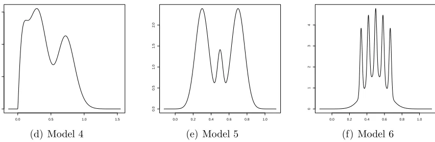
optimal bandwidths obtained from MISE and ISE criterion defined in (3) and (6). We have simulated six models with densities shown in Figure 1, some of them have been taken from Mammen et al. (2011) and others from Marron and Wand (1992) but rescaled to the interval [0,1]. We have chosen these models to cover a wide range of densities with different complexity levels, including different number of modes and asymmetry.

−0.5 0.0 0.5 1.0 1.5

0.0

0.5

1.0

1.5

2.0

(a) Model 1

−0.2 0.0 0.2 0.4 0.6 0.8 1.0 1.2

0.0

0.5

1.0

1.5

(b) Model 2

0.0 0.5 1.0 1.5 2.0

0.0

0.5

1.0

1.5

2.0

2.5

0.0 0.5 1.0 1.5

0.0

0.5

1.0

1.5

(d) Model 4

0.0 0.2 0.4 0.6 0.8 1.0

0.0

0.5

1.0

1.5

2.0

(e) Model 5

0.0 0.2 0.4 0.6 0.8 1.0

0

1

2

3

4

(f) Model 6

Figure 1: The six simulated densities in the finite sample study.

These six models are:

• Model 1: a Normal distribution N(0.5,0.22).

• Model 2: a trimodal mixture of three Normal distributions,N(0.25,0.0752_{),N(0.5,0.075}2₎

and N(0.75,0.0752) with coefficients 1₃.

• Model 3: a gamma distribution, Gamma(a, b), with a =b2 _{and b = 1.5 applied on}

5x with x∈_R+_.

• Model 4: a mixture of three gamma distributions, Gamma(ai, bi),i= 1, . . . ,3 with

ai =b2i, b1 = 1.5,b2 = 3 andb3 = 6 applied on 8x and x∈R+, with coefficients 1₃.

• Model 5: a mixture of three Normal distributions, N(0.3,₄₀3 2), N(0.7,₄₀32) and

N(0.5,₃₂12) with coefficients ₂₀9, ₂₀9 and ₁₀1 respectively.

• Model 6: a mixture of six Normal distributions,N(µi, σi2),i= 1, . . . ,6 withµ1 = 0.5,

µ2 = 1₃, µ3 = ₁₂5, µ4 = 1₂, µ5 = ₁₂7, µ6 = 2₃, σ1 = 1₈ and σi = ₈₀1, i = 2, . . . ,6 with

coefficients c1 = 1₂ and ci = ₁₀1 ,i= 2, . . . ,6.

We have simulated 1000 length-biased samples from each model considering sample sizes n = 50, 100, 200 and 500, using the Epanechnikov kernel. From these samples we have evaluated the performance of the bandwidth selectors through the following measures:

m1 = mean(ISE(ˆh)), m2 = std(ISE(ˆh)),

m3 = mean(ˆh−hISE), m4 = std(ˆh−hISE).

The first two measures, m1 and m2 are referred to the error of the estimation, so they

methods. Meanwhile, m3 and m4 measure respectively, the bias and variability of the

difference between the theoretical benchmark and the value selected by the proposals. This provides information about the way the methods are choosing the bandwidth parameter.

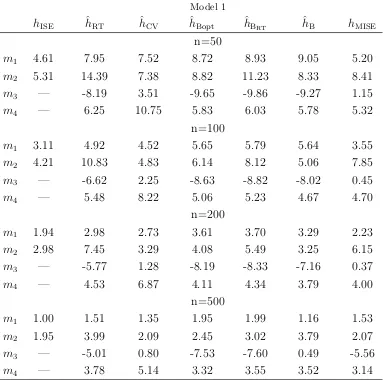
Table 1: Mean and standard deviations of the ISE and of the difference between the benchmark and the bandwidths selectors(criteria m1 to m4) for Model 1 multiplied by

102_.

Model 1

hISE hˆRT ˆhCV hˆBopt ˆhBRT ˆhB hMISE

n=50

m1 4.61 7.95 7.52 8.72 8.93 9.05 5.20

m2 5.31 14.39 7.38 8.82 11.23 8.33 8.41

m3 — -8.19 3.51 -9.65 -9.86 -9.27 1.15

m4 — 6.25 10.75 5.83 6.03 5.78 5.32

n=100

m1 3.11 4.92 4.52 5.65 5.79 5.64 3.55

m2 4.21 10.83 4.83 6.14 8.12 5.06 7.85

m3 — -6.62 2.25 -8.63 -8.82 -8.02 0.45

m4 — 5.48 8.22 5.06 5.23 4.67 4.70

n=200

m1 1.94 2.98 2.73 3.61 3.70 3.29 2.23

m2 2.98 7.45 3.29 4.08 5.49 3.25 6.15

m3 — -5.77 1.28 -8.19 -8.33 -7.16 0.37

m4 — 4.53 6.87 4.11 4.34 3.79 4.00

n=500

m1 1.00 1.51 1.35 1.95 1.99 1.16 1.53

m2 1.95 3.99 2.09 2.45 3.02 3.79 2.07

m3 — -5.01 0.80 -7.53 -7.60 0.49 -5.56

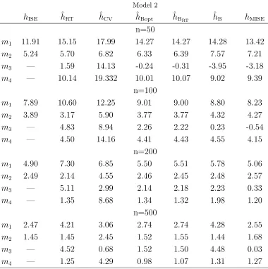
Table 2: Mean and standard deviations of the ISE and of the difference between the benchmark and the bandwidths selectors(criteria m1 to m4) for Model 2 multiplied by

102_.

Model 2

hISE ˆhRT hˆCV ˆhBopt hˆBRT ˆhB hMISE

n=50

m1 11.91 15.15 17.99 14.27 14.27 14.28 13.42

m2 5.24 5.70 6.82 6.33 6.39 7.57 7.21

m3 — 1.59 14.13 -0.24 -0.31 -3.95 -3.18

m4 — 10.14 19.332 10.01 10.07 9.02 9.39

n=100

m1 7.89 10.60 12.25 9.01 9.00 8.80 8.23

m2 3.89 3.17 5.90 3.77 3.77 4.32 4.27

m3 — 4.83 8.94 2.26 2.22 0.23 -0.54

m4 — 4.50 14.16 4.41 4.43 4.55 4.15

n=200

m1 4.90 7.30 6.85 5.50 5.51 5.78 5.06

m2 2.49 2.14 4.55 2.46 2.45 2.48 2.57

m3 — 5.11 2.99 2.14 2.18 2.23 0.33

m4 — 1.35 8.68 1.34 1.32 1.98 1.20

n=500

m1 2.47 4.21 3.06 2.74 2.74 4.28 2.55

m2 1.45 1.45 2.45 1.52 1.55 1.44 1.68

m3 — 4.52 0.68 1.52 1.50 4.48 0.03

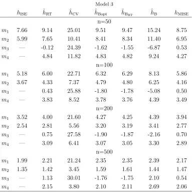
Table 3: Mean and standard deviations of the ISE and of the difference between the benchmark and the bandwidths selectors(criteria m1 to m4) for Model 3 multiplied by

102_.

Model 3

hISE ˆhRT ˆhCV ˆhBopt ˆhBRT ˆhB hMISE

n=50

m1 7.66 9.14 25.01 9.51 9.47 15.24 8.75

m2 5.99 7.65 10.41 8.41 8.34 11.40 6.95

m3 — -0.12 24.39 -1.62 -1.55 -6.87 0.53

m4 — 4.84 11.82 4.83 4.82 9.24 4.27

n=100

m1 5.18 6.00 22.71 6.32 6.29 8.13 5.86

m2 3.67 4.33 7.37 4.79 4.80 6.25 4.16

m3 — 0.43 25.88 -1.80 -1.78 -5.08 0.50

m4 — 3.83 8.52 3.78 3.76 4.39 3.49

n=200

m1 3.52 4.00 21.60 4.27 4.25 4.39 3.94

m2 2.54 2.81 5.56 3.20 3.19 3.41 2.77

m3 — 0.75 27.58 -1.90 -1.87 -2.16 0.70

m4 — 3.09 6.41 3.07 3.05 3.30 2.89

n=500

m1 1.99 2.21 21.24 2.35 2.35 2.39 2.17

m2 1.35 1.42 3.45 1.59 1.61 1.44 1.47

m3 — 1.13 30.01 -1.76 -1.75 2.10 0.54

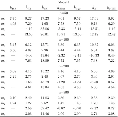
Table 4: Mean and standard deviations of the ISE and of the difference between the benchmark and the bandwidths selectors(criteria m1 to m4) for Model 4 multiplied by

102_.

Model 4

hISE hˆRT ˆhCV hˆBopt ˆhBRT ˆhB hMISE

n=50

m1 7.75 9.27 17.23 9.61 9.57 17.69 8.92

m2 4.93 7.20 4.65 7.58 7.59 9.13 6.29

m3 — -4.12 37.86 -5.33 -5.44 -15.51 -1.42

m4 — 13.53 26.01 13.71 13.66 12.12 12.47

n=100

m1 5.47 6.12 15.71 6.39 6.35 10.32 6.03

m2 3.56 4.07 2.96 4.44 4.44 5.81 3.87

m3 — -0.06 43.64 -2.32 -2.41 -10.33 0.49

m4 — 7.63 18.89 7.72 7.65 7.38 7.22

n=200

m1 3.68 4.13 15.22 4.16 4.16 5.63 4.09

m2 2.29 2.75 2.48 2.67 2.76 3.46 2.93

m3 — 1.65 48.79 -1.20 -1.33 -6.50 0.57

m4 — 4.61 13.04 4.53 4.50 5.08 4.54

n=500

m1 2.10 2.40 14.83 2.30 2.30 2.53 2.30

m2 1.24 1.27 2.62 1.42 1.43 1.70 1.46

m3 — 2.56 52.42 -0.62 -0.70 -2.32 0.27

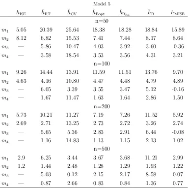
Table 5: Mean and standard deviations of the ISE and of the difference between the benchmark and the bandwidths selectors(criteria m1 to m4) for Model 5 multiplied by

102_.

Model 5

hISE ˆhRT ˆhCV ˆhBopt ˆhBRT hˆB hMISE

n=50

m1 5.05 20.39 25.64 18.38 18.28 18.84 15.89

m2 8.12 6.82 15.53 7.41 7.44 8.17 8.64

m3 — 5.86 10.47 4.03 3.92 3.60 -0.36

m4 — 3.58 18.54 3.53 3.56 4.31 3.21

n=100

m1 9.26 14.44 13.91 11.59 11.51 13.76 9.70

m2 4.63 4.16 10.80 4.47 4.48 4.79 4.89

m3 — 6.05 3.39 3.55 3.47 5.12 -0.16

m4 — 1.67 11.47 1.63 1.64 2.86 1.50

n=200

m1 5.73 10.21 11.27 7.19 7.26 11.52 5.92

m2 2.69 2.71 13.25 2.73 2.72 3.26 2.74

m3 — 5.65 5.36 2.83 2.91 6.44 -0.08

m4 — 1.16 14.83 1.13 1.15 2.13 1.02

n=500

m1 2.9 6.25 3.44 3.67 3.68 11.21 2.99

m2 1.2 1.44 2.48 1.28 1.29 1.93 1.22

m3 — 5.03 0.12 2.15 2.17 8.58 0.07

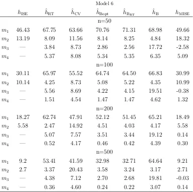
Table 6: Mean and standard deviations of the ISE and of the difference between the benchmark and the bandwidths selectors(criteria m1 to m4) for Model 6 multiplied by

102_.

Model 6

hISE hˆRT ˆhCV hˆBopt ˆhBRT ˆhB hMISE

n=50

m1 46.43 67.75 63.66 70.76 71.31 68.98 49.66

m2 13.19 8.09 11.56 8.14 8.25 4.84 18.32

m3 — 3.84 8.73 2.86 2.56 17.72 -2.58

m4 — 5.37 8.08 5.34 5.35 6.35 5.09

n=100

m1 30.11 65.97 55.52 64.74 64.50 66.83 30.99

m2 10.14 4.25 8.73 5.08 5.22 4.35 10.99

m3 — 5.56 8.69 4.22 4.15 19.51 -0.38

m4 — 1.51 4.54 1.47 1.47 4.62 1.32

n=200

m1 18.27 62.74 47.91 52.12 51.45 65.21 18.49

m2 5.58 2.47 14.92 4.51 4.03 4.17 5.58

m3 — 5.07 7.57 3.51 3.44 19.12 0.14

m4 — 0.52 4.17 0.46 0.42 4.39 0.30

n=500

m1 9.2 53.41 41.59 32.98 32.71 64.64 9.21

m2 2.7 3.37 20.43 3.58 3.24 3.17 2.71

m3 — 4.38 7.12 2.70 2.68 19.81 -0.03

m4 — 0.36 4.60 0.24 0.22 3.07 0.14

An overview of these numbers indicates that the performance of the methods depends on the complexity of the underlying model. Let classify the models in “easy” (Model 1, Model 3 and Model 4), “intermediate” (Model 2 and Model 5) and “hard” (Model 6) estimation problems.

Regarding to the measurem1, the rule-of-thumb performs better in smoother densities,

such as Model 1, Model 3 and Model 4, however the bootstrap bandwidths are also really competitive for these models, while cross-validation has in general a poorer performance. We have to remark that in Model 4, the bootstrap bandwidth ˆhB needs a large sample

size in order to be competitive. Increasing the complexity of the densities, Model 2 and Model 5, the performance of the rule-of-thumb decreases considerably and the bootstrap procedures ˆhBRT and ˆhBNS seems to be more accurate; however ˆhBhas a worse performance

on the design and the sample size, cross-validation can also produce competitive results. In hard estimation problems as Model 6, bootstrap bandwidths ˆhBRT and ˆhBNS are still

valuable competitors.

In terms of variability, which is measured by criterionm2 andm4, the cross-validation

method exhibits the highest values. The variability of the rule-of-thumb and the bootstrap bandwidths is in general moderate, with the only exception of ˆhB in Model 6 where it

exhibits higher values than the other bootstrap rules and the rule-of-thumb.

The bias in bandwidth selection is measured through m3. Rule-of-thumb and

boot-strap bandwidths with pilots generally show bias in the same direction and amount, except for Model 3 where they do not follow this pattern, even though the overall result is good. In smoother models both, tend to oversmooth and the opposite happens with cross-validation. The bias of the other bootstrap bandwidth selector, ˆhB, tends to be

higher except for very large sample sizes of Model 1.

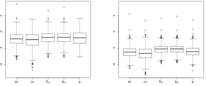
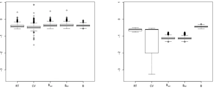
Moreover, the performance of all the methods proposed may also be compared graph-ically through the box plots of the errors (ISE’s) computed in the 1000 Monte Carlo samples (see Figures 2 - 7). These plots confirm that the behaviour of the selectors de-pends on the complexity of the underlying model. The bootstrap proposals seems to have in general a good behaviour outperformed only by cross-validation in Model 6, due to its complexity.

RT CV Bopt BRT B

−6

−4

−2

0

RT CV Bopt BRT B

−6

−4

−2

0

RT CV Bopt BRT B

−5

−4

−3

−2

−1

0

RT CV Bopt BRT B

−5

−4

−3

−2

−1

Figure 3: The plot of log(ISE) for the density estimation using the different bandwidth selectors for Model 2 and sizes n=50, 500 (from left to right).

RT CV Bopt BRT B

−6

−5

−4

−3

−2

−1

0

RT CV Bopt BRT B

−6

−5

−4

−3

−2

−1

0

Figure 4: The plot of log(ISE) for the density estimation using the different bandwidth selectors for Model 3 and sizes n=50, 500 (from left to right).

RT CV Bopt BRT B

−6

−5

−4

−3

−2

−1

RT CV Bopt BRT B

−6

−5

−4

−3

−2

−1

RT CV Bopt BRT B

−4

−3

−2

−1

0

RT CV Bopt BRT B

−4

−3

−2

−1

0

Figure 6: The plot of log(ISE) for the density estimation using the different bandwidth selectors for Model 5 and sizes n=50, 500 (from left to right).

RT CV Bopt BRT B

−3

−2

−1

0

1

RT CV Bopt BRT B

−3

−2

−1

0

1

Figure 7: The plot of log(ISE) for the density estimation using the different bandwidth selectors for Model 6 and sizes n=50, 500 (from left to right).

5

Conclusions

6

Further extensions

As we have remarked in Section 2, the methods presented in this paper can be easily generalised for a general known weight function ω, where the particular case of length-biased data is that ofω(y) =y. First, an appropriate modification of the estimator in (1) must be defined, as it has already been presented in Jones (1991):

ˆ

fh,ω(y) =

1

nµˆω

n

X

i=1

ω(Yi)−1Kh(y−Yi),

with ˆµω =

1

n

n

X

i=1

ω(Yi)−1

!−1

.

Theorem 2.1 and Corollary 2.2 can be generalised assuming the following conditions:

(B.1) E

1

ω(X)

<∞, E

1

ω(Y)l

<∞ l= 1, . . . ,2ν,

(B.2) R K(u)du= 1, R uK(u)du= 0 andµ2(K)<+∞

(B.3) limn→∞nh= +∞,

(B.4) y a continuity point off,

(B.5) f and ω are two times differentiable in y.

We immediately get the error measures as and their optimal bandwidth parameters for the length-biased data:

MSE( ˆfh,ω(y)) =

1 4h

4_f00

(y)2µ2₂(K) + γω(y)

nh R(K) +o

h4+ 1

nh

,

with γω(y) =

f(y)µω

ω(y) and

hAMSE,ω(y) =

γω(y)R(K)

n(f00(y))2_µ2 2(K)

1/5

.

We also obtain:

MISE( ˆfh,ω) =

1 4h

4

µ2₂(K)R(f00) + R(K)µωcω

nh +o

h4+ 1

nh

where cω =

Z

1

ω(y)f(y)dy and then

hAMISE,ω =

R(K)µωcω

nµ2

2(K)R(f

00

)

1/5

The bootstrap methods can be also modified in the same way. Then, the smooth bootstrap samples,Y₁∗, . . . , Y_n∗, can be generated by sampling randomly with replacement

n times from the estimated density ˆfY,g,ω(y) = ω(y) ˆfg,ω(y)/µˆω. Here g is again a pilot

bandwidth.

For the extension of the bandwidth selectors we need to take into account not only the above modification of the density estimator but also

ˆ

σ2_ω = 1

n

n

X

i=1

1

ω(Yi)

!−1



1

n

n

X

i=1

ω(Yi)

!

− 1

n

n

X

i=1

1

ω(Yi)

!−1

.

Apart from these considerations the procedures can be obtained in the same way as the length-biased case.

Acknowledgements

The authors are grateful for constructive comments from the associate editor and two reviewers which helped to improve the paper. They also acknowledge the support from the Spanish Ministry of Economy and Competitiveness, through grant number MTM2013-41383P, which includes support from the European Regional Development Fund (ERDF). Support from the IAP network StUDyS from Belgian Science Policy, is also acknowledged. M.I. Borrajo has been supported by FPU (FPU2013/00473) from the Spanish Ministry of Education.

References

Ahmad, I.A. (1995), ‘On multivariate kernel estimation for samples from weighted distri-butions’, Statistics & Probability Letters, 22, pp. 121–129.

Asgharian, M., M’Lan, C.E., and Wolfson, D.B. (2002), ‘Length-biased sampling with right censoring: an unconditional approach’,Journal of the American Statistical Asso-ciation, 97, pp. 201–209.

Barmi, H.E., and Simonoff, J.S. (2000), ‘Transformation-based density estimation for weighted distributions’,Journal of Nonparametric Statistics, 12, pp. 861–878.

Bhattacharyya, F.L.A., B, and Richardson, G.D. (1988), ‘A comparioson of nonpara-metric unweighted and length-biased density estimation of fibres’,Communications in Statistics-Theory and Methods, 17, pp. 3629–3644.

Bose, A., and Dutta, S. (2013), ‘Density estimation using bootstrap bandwidth selector’,

Bowman, A.W. (1984), ‘An alternative method of cross-validation for the smoothing of density estimates’,Biometrika, 71, 353–360.

Brunel, E., Comte, F., and Guilloux, A. (2009), ‘Nonparametric density estimation in presence of bias and censoring’,Test, 18, pp. 166–194.

Cacoullos, T. (1966), ‘Estimation of a multivariate density’, Annals of the Institute of Statistical Mathematics, 18, pp. 179–189.

Cao, R. (1990), ‘Aplicaciones y nuevos resultados del M´etodo Bootstrap en la estimaci´on no param´etrica de curvas’, Ph.D. dissertation, Universidade de Santiago de Compostela.

Cao, R. (1993), ‘Bootstrapping the mean integrated squared error’, Journal of Multivari-ate Analysis, 45, pp. 137–160.

Cao, R., Cuevas, A., and Gonz´alez-Manteiga, W. (1994), ‘A comparative study of several smoothing methods in density estimation’,Computational Statistics and Data Analysis, 17, pp. 153–176.

Chakraborty, R., and Rao, C.R. (2000), ‘23 Selection biases of samples and their resolu-tions’,Handbook of Statistics, 18, pp. 675–712.

Chesneau, C. (2010), ‘Wavelet block thresholding for density estimation in the presence of bias’, Journal of the Korean Statistical Society, 39, pp. 43–53.

Chiu, S.T. (1992), ‘An automatic bandwidth selector for kernel density estimation’,

Biometrika, 79, pp. 771–782.

Collomb, G. (1976), ‘Estimation non parametrique de la regression par la m´ethode du noyau’, Ph.D. dissertation, Universit Paul Sabatier de Toulouse.

Comte, F., and Rebafka, T. (2016), ‘Nonparametric weighted estimators for biased data’,

Journal of Statistical Planning and Inference, 174, pp. 104–128.

Cox, D. (2005), ‘Some sampling problems in technology’, in Selected Statistical Papers of Sir David Cox, Vol. 1, eds. D. Hand and A. Herzberg, Cambridge University Press, pp. pp. 81–92.

Cutillo, L., De Feis, I., Nikolaidou, C., and Sapatinas, T. (2014), ‘Wavelet density es-timation for weighted data’, Journal of Statistical Planning and Inference, 146, pp. 1–19.

de U˜na- ´Alvarez, J. (2004), ‘Nonparametric estimation under length-biased sampling and type I censoring: a moment based approach’, Annals of the Institute of Statistical Mathematics, 56, pp. 667–681.

Efromovich, S. (2004), ‘Density estimation for biased data’, Annals of Statistics, 32, pp. 1137–1161.

Gonz´alez-Manteiga, W., Mart´ınez-Miranda, M.D., and P´erez-Gonz´alez, A. (2004), ‘The choice of smoothing parameter in nonparametric regression through Wild Bootstrap’,

Computational Statistics and Data Analysis, 47, pp. 487–515.

Guillam´on, A., Navarro, J., and Ruiz, J.M. (1998), ‘Kernel density estimation using weighted data’,Communications in Statistics-Theory and Methods, 27, pp. 2123–2135.

Hall, P., and Marron, J.S. (1987), ‘Estimation of integrated squared density derivatives’,

Statistics & Probability Letters, 6, pp. 109–115.

Heckman, J.J. (1990), ‘Selection bias and self-selection’, in Econometrics, Springer, pp. pp. 201–224.

Heidenreich, N.B., Schindler, A., and Sperlich, S. (2013), ‘Bandwidth selection for ker-nel density estimation: a review of fully automatic selectors’, Advances in Statistical Analysis, 97, pp. 403–433.

Jones, M.C. (1991), ‘Kernel density estimation for length biased data’, Biometrika, 78, pp. 511–519.

Jones, M.C., and Karunamuni, R.J. (1997), ‘Fourier series estimation for length biased data’,Australian Journal of Statistics, 39, pp. 57–68.

Jones, M.C., Marron, J.S., and Sheather, S.J. (1996), ‘A brief survey of bandwidth se-lection for density estimation’,Journal of the American Statistical Association, 91, pp. 401–407.

Mammen, E., Mart´ınez-Miranda, M.D., Nielsen, J.P., and Sperlich, S. (2011), ‘Do-validation for kernel density estimation’, Journal of the American Statistical Associ-ation, 106, pp. 651–660.

Mammen, E., Mart´ınez-Miranda, M.D., Nielsen, J.P., and Sperlich, S. (2014), ‘Further theoretical and practical insight to the do-validated bandwidth selector’,Journal of the Korean Statistical Society, 43, pp. 355–365.

Marron, J.S. (1988), ‘Automatic smoothing parameter selection: a survey’, Empirical Economics, 13, pp. 187–208.

Marron, J.S. (1992), ‘Bootstrap bandwidth selection’, inExploring the limits of bootstrap, eds. R. Lepage and L. Billard, Wiley, pp. pp. 249–262.

Parzen, E. (1962), ‘On estimation of a probability density function and mode’,The Annals of Mathematical Statistics, 33, 1065–1076.

Patil, G.P., and Rao, C.R. (1977), ‘The weighted distributions: A survey of their appli-cations’,Applications of Statistics, 383, pp. 383–405.

Ram´ırez, P., and Vidakovic, B. (2010), ‘Wavelet density estimation for stratified size-biased sample’, Journal of Statistical Planning and Inference, 140, pp. 419–432.

Richardson, G.D., Kazempour, M.K., and Bhattacharyya, B. (1991), ‘Length biased den-sity estimation of fibres’,Journal of Nonparametric Statistics, 1, pp. 127–141.

Rosenblatt, M. (1956), ‘Remarks on some nonparametric estimates of a density function’,

The Annals of Mathematical Statistics, 27, pp. 832–837.

Rudemo, M. (1982), ‘Empirical choice of histograms and kernel density estimators’, Scan-dinavian Journal of Statistics, 9, pp. 65–78.

Scott, D.W. (1992), Multivariate density estimation: Theory, practice and visualisation, Wiley.

Sheather, S.J., and Jones, M.C. (1991), ‘A reliable data-based bandwidth selection method for kernel density estimation’,Journal of the Royal Statistical Society. Series B, 53, pp. 683–690.

Silverman, B.W. (1986),Density estimation for statistics and data analysis, CRC press.

Simon, R. (1980), ‘Length biased sampling in etiologic studies’, American Journal of Epidemiology, 111, pp. 444–452.

Turlach, B.A. (1993), ‘Bandwidth selection in kernel density estimation: A review’, Tech-nical report, Universit´e catholique de Louvain.

Vardi, Y. (1982), ‘Nonparametric estimation in the presence of length bias’, The Annals of Statistics, 10, pp. 616–620.

Vardi, Y. (1985), ‘Empirical distributions in selection bias models’, The Annals of Statis-tics, 13, pp. 178–203.

Zelen, M., and Feinleib, M. (1969), ‘On the theory of screening for chronic diseases’,

Appendices

A

Proof of Theorem 2.1

First of all we rewrite the estimator in (1) as follows:

ˆ

fh(y) =

1

n

1

1

n

Pn

i=n

1

Yi n

X

i=1

1

Yi

Kh(y−Yi) =

1

n

Pn

i=1

1

YiKh(y−Yi)

1

n

Pn

i=n

1

Yi

= φn(y)

ξn

. (7)

We start by calculating the punctual mean of (1) for which we need the mean of the numerator and denominator in (7), so:

φn(y) :=E[φn(y)] =E

"

1

n

n

X

i=1

1

Yi

Kh(y−Yi)

#

=

Z

1

zKh(y−z)fY(z)dz =

1

µ(Kh ◦f)(y).

ξn:=E[ξn] =E

"

1

n

n

X

j=1

1

Yj

#

=

Z

1

zfY(z)dz =

1

µ.

We divide this proof in two separated but linked paragraphs, detailing all the results involving mean and variance calculations respectively.

Mean

Applying the linearisation technique used in Collomb (1976) with ν ≥ 2 and taking into account that ξn6= 0∀n, we can write down

ˆ

fh(y) =

φn(y)

ξn

= φn(y)

ξn

· ξn

ξn

= φn(y)

ξn

"

1 +

ν−1

X

k=1

(−1)k

ξn−ξn

ξn

k

+ (−1)νξn

ξn

ξn−ξn

ξn

ν#

= φn(y)

ξn

"

1 +

ν−1

X

k=1

(−1)k

ξn−ξn

ξn

k#

+ (−1)νfˆh(y)

ξn−ξn

ξn

ν

.

Using the notationSa,b

n (y) :=E[φan(y)(ξn−ξn)b],sa,bn (y) :=E[(φn(y)−φn(y))a(ξn−ξn)b],

E[ ˆfh(y)] =E

"

φn(y)

ξn

+φn(y)

ξn

v−1

X

k=1

(−1)k

ξn−ξn

ξn

k

+ (−1)νfˆh(y)

ξn−ξn

ξn

ν#

= φn(y)

ξn

+

ν−1

X

k=1

(−1)kE[φn(y)(ξn−ξn)

k_]

ξn

k+1 +

(−1)ν

ξn

ν E[ ˆfh(y)(ξn−ξn)ν]

= φn(y)

ξn

+

ν−1

X

k=1

(−1)kS

1,k

n (y)

ξn

k+1 + (−1)

νσn1,ν(y)

ξn ν

= φn(y)

ξn

+ φn(y)S

0,2

n (y)−ξns1n,2(y)−ξnSn1,1(y)

ξn

3 +

ν−1

X

k=1

(−1)kS

1,k

n (y)

ξn

k+1 + (−1)

νσ1n,ν(y)

ξn ν

Then, we have proved that

E[ ˆfh(y)] =

φn(y)

ξn

+cn(y) +c(nν)(y) +

(−1)ν_σ1,ν

n (y)

ξn

ν ,

where

cn(y) =

φn(y)Sn0,2(y)−ξnSn1,1(y)

ξn

3 =

φn(y)E[(ξn−ξn)2]−ξnE[φn(y)(ξn−ξn)]

ξn

3 and

c(_nν)(y) = s

1,2

n (y)

ξn

3 +

ν−1

X

k=1

(−1)kS

1,k

n (y)

ξn

k+1 =

E[(φn(y)−φn(y))(ξn−ξn)2]

ξ3

n

+

+Pν−1

k=1(−1)

k E[φn(y)(ξn−ξn)k_]

ξnk+1 .

The first addend corresponds to the asymptotic expression of the mean obtained by Jones (1991). We want now to expand each of the other terms and study the rate of convergence. To this aim we use some basic statistical properties and we proceed as follows:

E(ξn−ξn)2

=V ar[ξn] =E

ξ_n2−ξn

2 =E     1 n n X j=1 1 Yj   2 − 1

µ2 =

1

n2E   n X i=1 1 Y2 j +X

i6=j

1 Yi 1 Yj  − 1 µ2 = 1

n2nE

1

Y2 1

+(n

2_−n)

n2 E 1 Y1 1 Y2 − 1

µ2 =

1

n

Z

1

z2g(z)dz+

n−1

n E 1 Y1 2 − 1 µ2 = 1 nE 1 X

+n−1

nµ2 −

1

µ2 =

E

φn(y)(ξn−ξn)

=E[φn(y)ξn]−ξnφn(y)

=E   1 n n X i=1 1 Yi

Kh(y−Yi)

!  1 n n X j=1 1 Yj    − 1

µ2(Kh◦f) (y)

= 1

n2E   n X i=1 1 Y2 i

Kh(y−Yi) +

X

i6=j

1

Yi 1

Yj

Kh(y−Yi)



−

1

µ2 (Kh∗f) (y)

= n

n2E

1

Y2 1

Kh(y−Y1)

+ n(n−1)

n2 E

1

Y1

1

Y2

Kh(y−Y1)

− 1

µ2(Kh◦f) (y)

= 1

nµ2 (Kh◦γ) (y)−

1

nµ2(Kh◦f) (y).

Hence,

cn(y) =µ3

1

µ(Kh◦f) (y)

1 nµ E 1 X − 1 µ − 1 µ 1

nµ2(Kh◦γ) (y)−

1

nµ2 (Kh◦f) (y)

= µ

n(Kh◦f) (y)

E 1 X − 1 µ

| {z }

(a)

−1

n(Kh◦γ) (y)

| {z }

(b)

+1

n(Kh◦f) (y)

| {z }

(c)

.

Applying Theorem 2.1 of Cacoullos (1966) with g(z) =f(z) for (a) and (c), and g(z) = f(_zz)

for (b), we easily obtain that every of these addends is O(1/n). Therefore, cn(y) =O(1/n).

To expand the next two terms we use the H¨older inequality and, taking into account that

K is bounded, we only require the finiteness of the second order moment of _Y1.

Ehφn(y) ξn−ξn

2i ≤E

φ2_n(y)1/2

Eh ξn−ξn

4i1/2

=O(1/n)1/2O(1/n2)1/2=O(1/n3/2)

Eh ξn−ξn

2i

=O(1/n).

Therefore,

c(_nν)(y) =O(1/n).

Finally,

σ_n1,ν(y) =E

h

ˆ

fh(y) ξn−ξn

νi ≤E h ˆ fh 2

(y)

i1/2

E

h

ξn−ξn

2νi1/2

=O(1)O(1/nν)1/2=O(1/nν/2).

Variance

To get the variance, we compute the expected value of the squared estimator. We follow the

same techniques as in the previous operations replacing ˆfh(y) by ˆfh

2

ˆ

fh

2

(y) =φ

2

n(y)

ξ2

n

= φ

2

n(y)

ξ2_n

· ξ 2

n

ξ2

n(y)

= φ

2

n(y)

ξ2_n



1 +

ν−1

X

k=1

(−1)k ξ

2

n(y)−ξ

2

n

ξ2_n

!k

+ (−1)νfˆh

2

(y) ξ

2

n(y)−ξ

2

n

ξ2_n

!ν

= φ

2

n(y)

ξ2_n



1 +

ν−1

X

k=1

(−1)k k

X

j=0

k!

j!(k−j)!2

k−j

ξn−ξn

ξ_n

k+j 

+

+ (−1)νfˆh

2

(y) ν

X

j=0

ν!

j!(ν−j)!2

ν−j

ξn−ξn

ξ_n

ν+j

.

To obtain the mean of ˆfh

2

(y) we need to work on S

2,l

n (y)

ξ2_n

= φ

2

ns

0,l

n (y) + 2φ

2

ns

1,l

n (y) +s2n,l(y)

ξ2_n

as follows:

Ehfˆh

2

(y)i= 1

ξ2_n E

φn(y)2

+E





φn(y)2(y)

ξ2_n

ν−1

X

k=1

(−1)k k

X

j=0

k!

j!(k−j)!2

k−j

ξn−ξn

ξ_n

k+j 

+

+ (−1)ν ν

X

j=0

ν!2ν−j

j!(ν−j)!

E

h

ˆ

fh

2

(y) ξn−ξn

ν+ji

ξν_n+j

= E

φ2_n(y)

ξ2_n +

ν−1

X

k=1

(−1)k k

X

j=0

k!

j!(k−j)!2

k−jS

2,k+j

n (y)

ξk_n+j+2

+ (−1)ν k

X

j=0

ν!

j!(ν−j)!2

ν−jσ

2,ν+j

n (y)

ξν_n+j

= φ

2

n

ξ2_n +

s0n,2(y)

ξ2_n +

ν−1

X

k=1

(−1)k k

X

j=0

k!

j!(k−j)!2

k−jφ

2

ns

0,k+j

n (y) + 2φns

1,k+j

n (y) +s2n,k+j(y)

ξk_n+j+2

+ (−1)ν ν

X

j=0

ν!

j!(ν−j)!2

ν+jσ

2,ν+j

n (y)

ξν_n+j

= φ

2

n

ξ2_n

+ s

2,0

n (y)

ξ2_n

−22φns

1,1

n (y) +s2n,1(y)

ξ3_n

−φ 2

ns

0,2

n (y) + 2φns

1,2

n (y) +s2n,2(y)

ξ4_n

+

+ 4φ

2

ns

0,2

n (y) + 2φns

1,2

m (y) +s2n,2(y)

ξ4_n + 4 Sn2,3(y)

ξ5_n +

Sn2,4(y)

ξ6_n +

+

ν−1

X

k=3

(−1)k k

X

j=0

k!

j!(k−j)!2

k−jS

2,k+j

n (y)

ξk_n+j+2

+ (−1)ν ν

X

j=0

ν!

j!(ν−j)!2

ν+jσ

2,ν+j

n (y)

ξν_n+j

= φ

2

n

ξ2_n

+ s

0,2

n (y)

ξ2_n

+ 3φns

0,2

n (y)

ξ4_n

−4φns

1,1

n (y)

ξ3_n

−2s

2,1

n (y)

ξ3_n

+

+ 3 s

2,2

n (y)

ξ4_n +

2φ_ns1n,2(y)

ξ4_n

!

+ 4S

2,3

n (y)

ξ5_n +

Sn2,4(y)

ξ6_n +

+

ν−1

X

k=3

(−1)k k

X

j=0

k!

j!(k−j)!2

k−jS

2,k+j

n (y)

ξk_n+j+2

+ (−1)ν ν

X

j=0

ν!

j!(ν−j)!2

ν+jσ

2,ν+j

n (y)

ξν_n+j .

Hence,

Ehfˆh

2

(y)i= φ

2

n(y)

ξ2_n

+ϕn(y) + Γ(nν)(y) + (−1)ν∆(ν)(y), where

ϕn(y) =

s0n,2(y)

ξ2_n

+ 3φns

0,2

n (y)

ξ4_n

−4φns

1,1

n (y)

ξ3_n

,

Γ(_nν)(y) =−2s

2,1

n (y)

ξ3_n

+ 3 s

2,2

n (y)

ξ4_n

+2φns

1,2

n (y)

ξ4_n

!

+ 4S

2,3

n (y)

ξ5_n

+S

2,4

n (y)

ξ6_n

+

+

ν−1

X

k=3

(−1)k k

X

j=0

k!

j!(k−j)!2

k−jS

2,k+j

n (y)

ξk_n+j+2

,

∆(ν)(y) = ν

X

j=0

ν!

j!(ν−j)!2

ν+jσ

2,ν+j

n (y)

ξν_n+j

.

As we have done before for the mean, we must study the convergence order of these terms.

s2_n,0(y) =Eh φn(y)−φn(y)

2i

=V ar[φn(y)] =E

φn(y)2

−φ_n(y)2

= 1

nµ2 K 2

h◦γ

(y) +n−1

nµ2 (Kh◦f) 2

(y)− 1

µ2 (Kh◦f) 2

(y)

= 1

nµ2 K 2

h◦γ

(y)− 1

nµ2(Kh◦f) 2

φ2_n(y)s_n0,2(y) =φ2_n(y)E

h

ξn−ξn

2i

=φ2_n(y) 1

nµ E 1 X − 1 µ = 1

nµ3 (Kh◦f) 2_(y)

E 1 X − 1 µ ,

φ_n(y)s1_n,1(y) =φ_n(y)E φn(y)−φn(y)

ξn−ξn

=φ_n(y)E

φn(y) ξn−ξn

−φ2_n(y)E

ξn−ξn

= 1

µ(Kh◦f) (y)

1

nµ2 (Kh◦γ) (y)−

1

nµ2(Kh◦f) (y)

= 1

nµ3(Kh◦f) (y) (Kh◦γ) (y)−

1

nµ3 (Kh◦f) 2_(y),

s2_n,1(y) =Eh φn(y)−φn(y)

2

ξn−ξn

i

=O(1/n)− 1

nµ3(Kh◦γ) (y)−

1

nµ3 (Kh◦f) 2_(y),

s2_n,2(y) =Eh φn(y)−φn(y)

2

ξn−ξn

2i

≤Eh φn(y)−φn(y)

4i1/2

Eh ξn−ξn

2i1/2

=O(1/n)O(1/n1/2) =O(1/n3/2).

In the same way as with this last term and assuming that the l-th order centred moment of

the variable _Y1 <+∞ withl= 1, . . . ,2ν, we obtain

φ_n(y)s_n1,2(y) =O(1/n3/2), S_n2,3(y) =O(1/n5/2), S_n2,4(y) =O(1/n3), S_n2,k+j(y) =O(1/nk+2j+1)

and σ_n2,ν+j(y) =O(1/nν+j).

Finally, gathering all the addends properly, we get

E

h

ˆ

fh

2

(y)

i

= φ

2

n(y)

ξ2_n

+ϕn(y) + Γ(nν)(y) + (−1)ν∆(ν)(y)

= (Kh◦f)2(y) + 1

n K

2

h◦γ

(y)− 1

n(Kh◦f)

2_(y).

Then,

V ar

h

ˆ

fh(y)

i

= (Kh◦f)2(y) + 1

n K

2

h◦γ

(y)− 1

n(Kh◦f)

2

(y)−(Kh◦f)2(y) +O(1/n)

= 1

n

h

K_h2◦γ

(y)−(Kh◦f)2(y)

i

+O(1/n)

To get the MSE it is enough to realise that

MSE

ˆ

fh(y)

= Bias2

ˆ

fh(y)

+ Var

ˆ

fh(y)

,

and apply a Taylor expansion as it is done with the kernel density estimator with complete data, then:

MSE

ˆ

fh(y)

= 1

4h

4_f00_(y)2_µ2 2(K) +

γ(y)

nh R(K) +o

h4+ 1

nh

B

Proof of Theorem 2.3

We now obtain the MSE of the bootstrap estimator under the bootstrap distribution. To this aim we follow similar steps as in Appendix A. Remind that now, the estimator is given by (5), and it can be rewritten as follows:

ˆ

fh

∗

(y) =

1

n

Pn

i=1

1

Y_i∗Lh(y−Y

∗

i )

1

n

Pn

j=1 Y1_j∗

= φ

∗

n(y)

ξ∗

n

.

From the expression above we compute the mean of the numerator and the denominator as follows:

φ∗_n(y) :=E∗[φ∗_n(y)] =E∗

" 1 n n X i=1 1

Y_i∗Lh(y−Y

∗ i ) # = Z 1

zLh(y−z) ˆfY,g(z)dz =

1 ˆ

µ

Lh◦fˆg

(z).

ξ∗_n:=E∗[ξ_n∗] =E∗

  1 n n X j=1 1

Y_j∗



= Z

1

zfˆY,g(z)dz =

1 ˆ

µ.

Using the linearisation procedure in Collomb (1976) with ν≥2 we have that

E∗[ ˆfh

∗

(y)] = φ

∗

n(y)

ξ∗_n +c

∗

n(y) +c∗

(ν)

n (y) +

(−1)νσ_n∗1,ν(y)

ξν_n where

c∗_n(y) =φ

∗

n(y)S∗

0,2

n −ξ

∗

nS∗

1,1

n

ξ∗_n3

=

φ∗_n(y)E∗

ξ_n∗−ξ∗_n2

−ξ∗_nE∗hφ∗_n(y)ξ∗_n−ξ∗_ni ξ∗_n3

,

c∗_n(ν)(y) = s

∗1,2

n (y)

ξ∗_n3

+

ν−1

X

k=3

(−1)kS

∗1,k

n (y)

ξ∗_nk+1

=

E∗

φ∗_n(y)−φ∗_n(y) ξ_n∗−ξ∗_n

2

ξ∗_n3

+

+Pν−1

k=3(−1)k

E∗hφ∗n(y)(ξ∗n−ξ

∗

n) ki

ξ∗n

k+1 and

σ_n∗1,ν(y) =E∗hfˆh

∗

(y)ξ_n∗−ξ∗_nνi

To obtain the variance of the bootstrap estimator we compute

E∗[ ˆfh

∗2

(y)] = φ

∗2

n (y)

ξ∗_n2

+ϕ∗_n(y) + Γ∗_n(ν)(y) + (−1)ν∆∗(ν)(y),

with

ϕ∗_n(y) = s

∗2,0

n (y)

ξ∗_n2

+ 3φn

∗2

(y)s∗_n0,2 ξ∗_n4

−4φ

∗

n(y)s∗

1,1

n

Γ∗_n(ν)(y) =−2s

∗2,1

n (y)

ξ∗_n3

+ 3 s

∗2,2

n (y)

ξ∗_n4

+2φ

∗

n(y)s∗

1,2

n

ξ∗_n4

!

+ 4S

∗2,3

n (y)

ξ∗_n5

+ S

∗2,4

n (y)

ξ∗_n6

+

+Pν−1

k=3(−1)k

Pk

j=0

k!2k−j

j!(k−j)!

Sn∗2,k+j(y)

ξ∗n

k+j+2 and

∆∗(ν)(y) = ν

X

j=0

ν!

j!(ν−j)!2

ν−jσ∗

2,ν+j

n (y)

ξ∗_nν+j .

Here the dominant terms are φ

∗2

n(y)

ξ∗_n2

+s

∗2,0

n (y)

ξ∗_n2

, which are the ones we need to study.

φ∗

2

n(y)

ξ∗_n2

=

1 ˆ

µ(Lh◦fˆg)(y)

2 1 ˆ µ 2

s∗_n2,0(y) =E∗

φ∗_n(y)−φ∗_n(y)2

=V ar∗[φ∗_n(y)] =E∗hφ_n∗2(y)i−E∗[φ∗_n(y)]2

=E∗

h

φ∗_n2(y)

i −φ∗

2

n(y) =

1

nµˆ2(L 2

h◦γˆg)(y) +

n−1

nµˆ2 (Lh◦fˆg)

2_(y)− 1

ˆ

µ2(Lh◦fˆg) 2_(y)

= 1

nµˆ2(L 2

h◦γˆg)(y)−

1

nµˆ2(Lh◦fˆg) 2_(y)

⇒ s

∗2,0

n (y)

ξ∗_n2

= ˆµ2s∗_n2,0(y) = 1

n(L

2

h◦γˆg)(y)−

1

n(Lh◦fˆg)

2_(y),

taking into account that E∗[φ∗_n2(y)] = 1

nµˆ(L

2

h◦γˆg)(y) +

n−1

nµˆ2 (Lh◦fˆg) 2_(y).

Then, as the other terms are negligible, we get

V ar∗hfˆh

∗

(y)i= 1

n

h

(L2_h◦γˆg)(y)−(Lh◦fˆh)2(y)

i

.

Under the regularity conditions previously established we get that

MSE∗( ˆfh

∗

(y)) = 1 4h

4_fˆ

g

00

(y)

2

µ2₂(K) +γˆg(y)

nh R(L) +oP

h4+ 1

nh

.

C

Proof of Theorem 2.6

This proof has basically the same aim as the one of Theorem 2.3 (Appendix B), with the particularity that the generation of the bootstrap sample is made differently.

Let us remind the expression of the bootstrap estimator

ˆ

fh

∗

(y) =

1 n Pn i=1 1 Y∗

i Lh(y−Y

∗

i )

1

n

Pn

j=1 Y1_j∗

= φ

∗

n(y)

ξ∗

n

.

φ∗_n(y) :=E∗[φ∗_n(y)] =E∗

"

1

n

n

X

i=1

1

Y_i∗Lh(y−Y

∗

i )

#

=

Z ₁

zLh(y−z) ˜fK,g(z)dz.

ξ∗_n:=E∗[ξ_n∗] =E∗





1

n

n

X

j=1

1

Y_j∗



= Z ₁

z

˜

fK,g(z)dz.

Remind that in this context, ˜fK,g denote the common kernel density estimator with kernel K

and bandwidth g.

Hence,

E∗hfˆ_h∗(y)i= φ

∗

n(y)

ξ∗_n +OP (1/n) =

R ₁

zLh(y−z) ˜fK,g(z)dz

R ₁

zf˜K,g(z)dz

+OP (1/n).

To compute the variance we follow again the previous proof, and taking only into account the dominant terms we get

E∗[ ˆfh

∗2

(y)] = φ

∗2

n (y)

ξ∗_n2

+s

∗2,0

n (y)

ξ∗_n2

+OP(1/n), where

φ∗

2

n(y)

ξ∗_n2

=

R ₁

zLh(y−z) ˜fK,g(z)dz

2

R ₁

zf˜K,g(z)dz

2 and

s∗_n2,0(y) =E∗

φ∗_n(y)−φ∗_n(y)2

=V ar∗[φ∗_n(y)] =E∗hφ_n∗2(y)i−E∗[φ∗_n(y)]2

=E∗hφ∗_n2(y)i−φ∗

2

n (y) =

1

n

Z ₁

z2L 2

h(y−z) ˜fK,g(z)dz−

1

n

Z ₁

zLh(y−z) ˜fK,g(z)dz

2

,

considering thatE∗[φ∗_n2(y)] = 1

n

Z

1

z2L 2

h(y−z) ˜fK,g(z)dz−

n−1

n

Z

1

zLh(y−z) ˜fK,g(z)dz

2

.

Then we get

V ar∗

h

ˆ

fh

∗

(y)

i

= 1

n

Z

1

z2L 2

h(y−z) ˜fK,g(z)dz−

1

n

Z ₁

zLh(y−z) ˜fK,g(z)dz

2

.

Finally, just noting that MSE∗ can be computed as the sum of the squared bias and the