Penalty-free feasibility boundary convergent multi-objective evolutionary algorithm for the optimization of water distribution systems

Penalty-Free Feasibility Boundary Convergent Multi-Objective Evolutionary Algorithm for the Optimization of Water Distribution Systems

Calvin Siew1 and Tiku T. Tanyimboh2

Department of Civil Engineering, University of Strathclyde Glasgow. John Anderson Building, 107 Rottenrow, Glasgow G4 0NG, UK.

1 _{PhD student, Department of Civil Engineering, University of Strathclyde Glasgow.}

John Anderson Building, 107 Rottenrow, Glasgow G4 0NG, UK. Email : [email protected]

Tel : +44 (0) 141 548 3578

2

Senior Lecturer (Corresponding Author), Department of Civil Engineering, University of Strathclyde Glasgow. John Anderson Building, 107 Rottenrow, Glasgow G4 0NG, UK.

Email : [email protected] Tel : +44 (0) 141 548 4366 Fax +44 (0) 141 553 2066

This article was published in Water Resources Management (2012) 26:4485–4507. DOI 10.1007/s11269-012-0158-2.

Water Resources Management

December 2012, Volume 26, Issue 15, pp 4485-4507

Penalty-Free Feasibility Boundary Convergent Multi-Objective Evolutionary Algorithm for the Optimization of Water Distribution Systems

Calvin Siew, Tiku T. Tanyimboh

The final publication is available at www.springerlink.com;

Penalty-Free Feasibility Boundary Convergent Multi-Objective Evolutionary Algorithm for the Optimization of Water Distribution Systems

Calvin Siew and Tiku T. Tanyimboh

Department of Civil Engineering, University of Strathclyde Glasgow, UK

Abstract

This paper presents a new penalty-free multi-objective evolutionary approach (PFMOEA) for the optimization of water distribution systems (WDSs). The proposed approach utilizes pressure dependent analysis (PDA) to develop a multi-objective evolutionary search. PDA is able to simulate both normal and pressure deficient networks and provides the means to accurately and rapidly identify the feasible region of the solution space, effectively locating global or near global optimal solutions along its active constraint boundary. The significant advantage of this method over previous methods is that it eliminates the need for ad-hoc penalty functions, additional “boundary search” parameters, or special constraint handling procedures. Conceptually, the approach is downright straightforward and probably the simplest hitherto. The PFMOEA has been applied to several WDS benchmarks and its performance examined. It is demonstrated that the approach is highly robust and efficient in locating optimal solutions. Superior results in terms of the initial network construction cost and number of hydraulic simulations required were obtained. The improvements are demonstrated through comparisons with previously published solutions from the literature.

1 Introduction

The computational complexity involved in optimizing the design and rehabilitation of water distribution systems (WDSs) is exceptionally high. Simply the selection of pipe diameters (from a set of commercially available discrete diameters) to form a water supply system of least capital cost has been demonstrated to be an NP-hard problem, let alone considering multiple loading conditions, operating cost, rehabilitation options and other aspects that affect real-life networks.Yates et al. (1984) stated that the global optimum solution to WDS design problem can only be guaranteed by means of explicit or implicit enumeration techniques such as dynamic programming. These techniques require a great amount of computer time as they involve searching the entire solution space. For example, a small eight-pipe network with 10 possible pipe sizes has a total of 108 feasible and infeasible pipe size combinations. It is clear that the search space increases exponentially with the size of the network. This undoubtedly marks the limitations of exhaustive enumeration techniques in optimizing realistic WDSs.

Alperovits and Shamir (1977) solved the highly nonlinear WDS design optimization problem by employing linear programming (LP). The LP formulation is based on a set of assumed pipe flow rates and pipe lengths are used as decision variables, resulting in designs in which pipes are made up of two-diameter segments. This type of solution is unfortunately unsuitable for practical implementation. Several researchers (e.g. Su et al. 1987; Lansey and Mays 1989) applied non-linear programming (NLP) in the design optimization of WDSs. However, the resulting NLP solutions are of continuous diameter values which are not directly applicable. Rounding the diameters up or down to the nearest discrete pipe sizes will not necessarily guarantee the optimality of the solution and can often deteriorate the quality of the solution. Moreover, the rounded solution may not even satisfy the pressure constraints and additional simulations are required to evaluate them. In general, mathematical programming methods rely on the initial solution and do not guarantee that the global optimum will be obtained. They are often trapped in local optima, resulting in suboptimal solutions. Also, this deterministic method is rigid and lacks flexibility as it only yields a single final solution.

Many developments have been carried out to improve the effectiveness and efficiency of GAs in the optimization of WDSs. Savic and Walters (1997) proposed the use of Gray coding as opposed to binary coding to overcome convergence problems related to the hamming cliff effect. Vairavamoorthy and Ali (2000) avoided the encoding and decoding of diameter variables by implementing real coding. Halhal et al. (1997) and Wu and Simpson (2001) used messy GA with variable length string representation. Vairavamoorthy and Ali (2000) reduced the computational time of the GA search by approximating the hydraulic behaviour of the WDS using a linear transformation function. Search space reduction was attempted by Vairavamoorthy and Ali (2005) and Mahendra et al. (2008) by limiting the candidate diameter for each link based on the pipe index vector and critical path method respectively. Keedwell and Khu (2006) enhanced the GA search by seeding the initial GA population with good solutions generated from a deterministic model based on a computational method known as cellular automaton.

In this paper, a new multi-objective evolutionary optimization approach for WDSs is proposed. The new approach employs a novel boundary-convergent technique which efficiently guides the search to concentrate on solutions close to the boundaries of the feasible region of the solution space. Also, a new rigorous and efficient way of handling constraints is introduced. The method developed herein completely eliminates the need for penalties. With proper assessment of the performance of near-feasible solutions in particular, the proposed approach is able very quickly to locate global or near global optimal solutions. Herein, the numbers of function evaluations required has been reduced by a very large margin in comparison to the best results for the benchmarks in the literature.

2 Constraint Handling

In general, trial solutions (WDS designs) generated by an EA are simulated using a hydraulic simulator and the resulting nodal heads are evaluated based on the pressure constraint requirements. Solutions that violate the pressure constraints are considered as infeasible. However, a major disadvantage of EAs is that they are unable to directly handle constraints. In other words, EAs are incapable of differentiating feasible solutions from non-feasible ones. Majority of the WDS EA optimization work in the literature use the penalty function approach to handle pressure constraints (e.g. Savic and Walters, 1997). In this method, an additional penalty cost is applied to the actual WDS cost of the infeasible solution. The penalty cost is usually calculated using penalty parameters which are formulated such that greater constraint violations incur higher penalty costs. In this way, the probability of solutions being discarded in the next generation will depend on their degree of constraint violation.

and exhaustive fine tuning before the penalty function can be effectively incorporated into the EA framework. Moreover, the effectiveness of the penalty parameters is often case sensitive in that the performance varies from one optimization problem to another. If poorly chosen, the penalty parameter can severely distort the objective function and impair the EA in terms of the optimality of the final solution and rate of convergence. Also, the unconstrained optimization problems generated by the penalty functions have larger objective function spaces compared to the original problems which, therefore, decrease the probability of the search to locate the optimum solution.

Several researchers have attempted to address this problem. Khu and Keedwell (2005) avoided the use of penalty functions by formulating each nodal pressure constraint as an objective function within a multi-objective evolutionary algorithm framework. This approach requires enormous computational effort and lacks the practicality to be applied to real-life WDSs which may contain hundreds or thousands of nodes. Following Deb (2000), Prasad and Park (2004) adopted a constraint handling method that does not require a penalty coefficient. This method uses a tournament selection operator where 1) feasible solutions are preferred over infeasible solutions; 2) between two infeasible solutions, the one with smaller constraint violation is selected; and 3) between two feasible solutions, the one with better fitness value is selected. A closer examination of the approach reveals that it can lead to anomalies. For example, the most expensive feasible solution will be ranked more highly than a borderline infeasible solution which may still be acceptable in reality and carry the overwhelming majority of the good genes.

Based on the fact that optimal or near-optimal solutions are generally located near the active constraint boundaries, Wu and Walski (2005) developed a self-adaptive penalty method based on a heuristic boundary search technique. The approach involved an evolving penalty factor that aimed to focus the GA search around the boundary of the feasible solution region. However, the implementation of this self-adaptive heuristic technique requires the prior calibration of several additional special parameters. Afshar and Marino (2007) proposed a self-adaptive penalty method. The approach incorporates a procedure that handles the constraints that are violated in an explicit way. Farmani et al. (2005) used a self-adaptive fitness formulation which involves the implementation of a two-stage penalty. The first stage ensures that the worst infeasible solution is allocated a penalty cost that is higher or at least equal to the cost of the cheapest feasible solution in the population. The penalty cost of the worst infeasible solutions is then further increased to twice the cost of the cheapest feasible solution at the second stage. However, the robustness of the suggested scheme is questionable as it can allow infeasible solutions to be selected over feasible solutions that cost more than twice the cost of the cheapest feasible solution.

Due to the assumption that nodal demands are fully satisfied regardless of whether the system’s pressure is sufficient or deficient, demand driven analysis (DDA) is incapable of depicting the actual performance of a pressure deficient network, i.e. the exact nodal outflow cannot be quantified. The DDA pressure heads do not accurately represent the actual deficiency of the network. In fact, resulting pressure heads are often lower or even unrealistically large negative values, leading to an exaggeration of the network pressure deficiency. For example, a nodal demand that is approximately 90% satisfied may still have a negative pressure head (Siew and Tanyimboh, 2011), giving a false impression that the nodal flow is zero. This once again highlights the complication and complexity involved in calibrating the penalty parameter. It is clear that the EA search can be easily misled if penalty parameters are not chosen properly. This paper presents a rigorous new approach that eradicates all the above mentioned difficulties. The use of penalty functions or other special constraint-handling techniques is obviated by involving a pressure dependent analysis (PDA) within a multi-objective optimization search. PDA (Tanyimboh et al. 1999) considers the relationship between pressure and nodal flow explicitly. The actual nodal flows and heads for both normal and pressure deficient networks can be simulated. This enables a more precise performance assessment of both feasible and infeasible solutions thus providing a far more robust means of steering the EA search toward the boundary between infeasible and feasible regions. The approach is referred to as the Penalty-Free Multi-Objective Evolutionary Algorithm (PFMOEA) herein. The PFMOEA does not involve any parameters that require prior calibration and its application has proven to be robust and effective in leading the GA search to locate optimal or near optimal solutions. The next sections describe the PDA hydraulic simulator (in brief) and the multi-objective optimization method used in this approach.

3 Pressure Dependent Analysis

A description of EPANET-PDX, with reference to EPANET 2 and the global gradient algorithm (Todini and Pilati 1988), and a review of PDA methods are available in Siew and Tanyimboh (2012). Also, a comparative analysis of several DDA computational solution methods for gas and water distribution networks is available in Brkic (2011). Recently Spiliotis and Tsakiris (2011) proposed a DDA implementation of the Newton-Raphson method using a pipe discharge formula derived by combining the Darcy-Weisbach pipe friction head loss formula and the Colebrook-White function for the friction factor (see e.g. Eq. 4.16 in Chadwick et al. 2004). The procedure (Brkic 2012, Spiliotis and Tsakiris 2012a) has the advantages that it avoids the iterative solution of the Colebrook-White function and benefits from the extra accuracy of the Darcy-Weisbach pipe friction head loss formula compared to empirical approximations such as the Hazen-Williams formula. It should be noted that the design optimization approach proposed here follows the convention that demands are known with reasonable certainty. Procedures that address uncertainties in the demands and other relevant parameters (Kumar et al. 2010, Spiliotis and Tsakiris 2012b) are not considered here.

We implemented the above-mentioned enhancements directly as additional subroutines within the EPANET 2 source code without involving any program interface or toolkit. It is worth mentioning that the full functionality of EPANET 2 is preserved. EPANET-PDX is highly robust and accurate in analyzing both normal and pressure deficient conditions. In terms of efficiency, extensive testing has shown that the computational performance of EPANET-PDX compares very favourably to EPANET 2 (Siew and Tanyimboh, 2011). With this said, one should bear in mind that EPANET 2 results are inaccurate, misleading or infeasible while analysing pressure deficient networks (Siew and Tanyimboh, 2011). The accuracy of the pressure dependent analysis results that EPANET-PDX produces has been validated and verified. The details can be found in Siew and Tanyimboh (2010).

4 Penalty-Free Boundary-Convergent Multi-Objective Optimization Method The optimization of an engineering design involves multiple objectives which are often contradicting. For example, to maximise the available flow of the network and minimize its capital cost simultaneously are obviously opposing objectives. The presence of these objectives gives rise to a set of compromised solutions known as the Pareto-optimal or non-dominated solutions in which no one solution in this set can be deemed to be superior over the others. The goal in a multi-objective optimization is to find as many diverse Pareto-optimal solutions as possible after which a higher-level decision is required to select one of them for implementation.

solutions belonging to the best non-dominated front of the combined population, and then subsequent non-dominated fronts in the order of their ranking. The last accepted front may contain more solutions than required to achieve a population of size N. If this occurs, the last front is sorted using a crowding distance operator that favours solutions with high diversity. This algorithm is repeated for several generations until a convergence criterion is satisfied. A detailed description of NSGA-II can be found in Deb et al. (2002).

We wrote a basic NSGA II program in C++ language and coupled it directly to EPANET-PDX. The NSGA II model is binary coded and utilizes simple GA operators such as single bit-wise mutation, single point crossover and a simple tournament selection. This enables the performance of the proposed approach to be effectively gauged without involving any EA convergence enhancing operators. The proposed approach involves two primary objectives. The first objective is to minimise the network capital cost. The second objective is to ensure all nodal demands are satisfied. This is achieved by maximizing the total available flow of the most critical node in the network. Network costs normally fall in the range of millions while nodal outflow values are comparatively much smaller and may vary depending on the size of the network and mathematical units used. Due to the vast difference between the objective function values, directly applying both the network cost and the available flow as objective functions may yield technical hitches during the crowding distance comparison sorting stage of the NSGA II. This can potentially result in a biased judgement of distance for the solutions. To overcome this, both objective functions are normalised.

Also, a new efficient boundary search technique was introduced to focus the PFMOEA search on near feasible solutions. This is done by exponentiating the 1st and 2nd objective functions as shown in Equations 2 and 3 respectively. It is important to note that the exponent values remain the same throughout the optimization search. Hence, the objective functions for the PFMOEA are formulated as:

Minimise

(

)

1 CR

F = (2)

Maximise F2 =

(

)

where F1 and F2 represent the first and second objective functions respectively; CR represents the cost ratio which can be expressed as:

max net

net C

C

CR= (4)

req i i crit

crit crit

Qn Qn

DSR = (5)

where

crit

i

Qn and req icrit

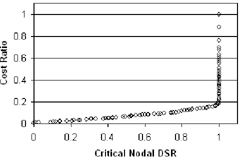
Qn are the actual flow and demand for the critical node icrit. This way, both objective functions are normalised and have values between 0 and 1.0. Fig. 1a and Fig. 1b show typical Pareto-optimal fronts of the PFMOEA with and without the implementation of the boundary search respectively. It is worth observing that the former possesses a more enhanced front that is denser with solutions near the boundary region compared to the latter which has quite a uniform spread of diverse solutions encompassing a wider range of DSR and contains a much higher proportion of infeasible solutions. The boundary search approach applied here is only at its preliminary phase. More work is required to further develop the method.

(Fig. 1a and Fig. 1b here)

In the advanced stages of the evolutionary process, after merging the parent and child populations (each of which has size N), the number of solutions belonging to the Pareto-optimal front (best non-dominated front) may exceed the number of solutions required to maintain a population of size N. Since all solutions residing in the same front are assumed (by NSGA II) to have the same quality, to select exactly N population members, these solutions are sorted using the crowding distance operator and solutions with the lowest crowding distance (i.e. solutions located in crowded regions) are eliminated. This results in a front with a uniform spread of diverse solutions consisting of numerous highly infeasible solutions on one hand and numerous highly redundant solutions on the other hand. This approach totally contradicts the desirable effect of the boundary search strategy (i.e. a Pareto-optimal front with solutions highly concentrated near the boundary of the feasible region as shown in Fig. 1a) and potentially leads to the elimination of some of the best solutions.

In the PFMOEA approach, 30% of the population consisting of the best (i.e. the least-cost feasible) solutions in each generation are retained by assigning them each with an extremely high crowding distance value. The remaining solutions are subjected to the crowding distance operator for selection to fill the remaining population slots. In this way, feasible solutions near the boundary region are preserved and diversity amongst the population members is still maintained to a certain extent. For example, consider a hypothetical PFMOEA search with a fixed population size of 100 and a set of 120 solutions in the best non-dominated front at the end of a generation. If there are 50 feasible solutions available, the cheapest 30 (i.e. 30% of 100) will be retained. 70 solutions out of the remaining 90 will then be selected based on their crowding distance to be combined with the 30 best solutions retained, forming a population size of 100 to be carried forward to the next generation.

energy conservation constraint requires that the total head loss along a path should be equal to the difference in head between its starting and ending nodes. Herein, the Hazen-Williams (HW) equation is used to approximate the head loss and can be described as:

b j a

j j j j

D C Qp L

h _ 1

     

=ω (6)

in which ω _{is a dimensionless conversion factor whose numerical value depends on}

the units used; hj, Lj, Qpj, Cj and Dj represent the head loss, length, flow rate, HW

coefficient and internal diameter for pipe j respectively; a and b are coefficients with values 1.852 and 4.870 respectively.

Several researchers use different conversion factors ω_{. Similarly to Savic and Walters}

(1997), with the purpose of covering the range of published values and enabling a rigorous comparison of optimal solutions obtained by other researchers in the literature, results presented in this paper are based on two ω _{values i.e. 10.5088 and}

10.9031.

5 Examples, Results and Discussion

The PFMOEA is applied to three well known optimization problems, i.e. the design of the Two-Loop and Hanoi WDSs, and the expansion of the New York Tunnels (Fig. 2a, Fig. 2b and Fig. 2c respectively). It is no doubt that the three benchmarks are simple and do not fully depict the actual problems of real-world WDSs. However, these networks have been extensively analyzed by numerous researchers using various methods and hence, the comparison of the PFMOEA results to the best optimum solutions obtained from the literature would serve as a good ground in demonstrating the effectiveness of the proposed optimization approach. It is worth clarifying that no attempt was made to optimize the mutation rate herein. For the three examples presented, the mutation rates applied vary from 0.005 to 0.02 based on typical values obtained from the literature.

(Fig. 2a, Fig. 2b and Fig. 2c here)

5.1 Two-Loop Network

Fig. 2a shows the layout of the Two-Loop network. This single source network consists of eight pipes of length 1000m and six demand nodes. The minimum pressure requirement for all nodes is defined as 30m. An HW roughness coefficient of 130 is used for new pipes. A set of 14 commercial pipe diameters is used in this design optimization problem. The diameters and costs of these pipes and node data can be found in Alperovits and Shamir (1977).

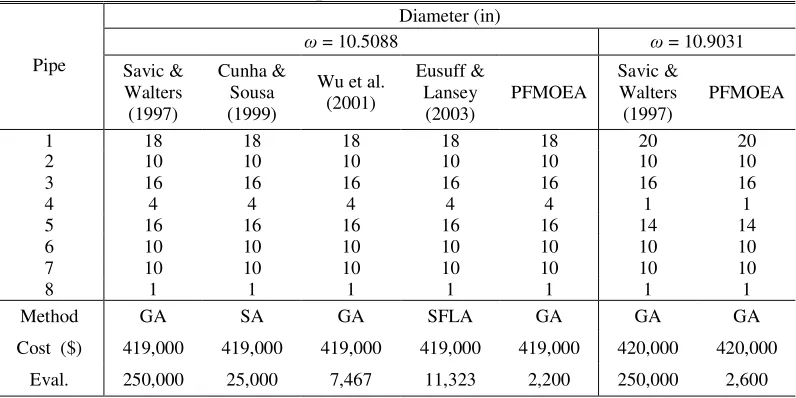
Solutions found in previous studies are presented in Table 1. Additional studies can be found in Ekinci and Kunak (2009). Results, i.e. pipe diameters are presented in imperial units to enable an easy comparison. Savic and Walters (1997) were probably the only researchers who reported the solution with ω_{=10.9031; their least cost}

solution of $420,000 was obtained within a total of 250,000 function evaluations. For this small network, it took the PFMOEA only 10 random runs each (i.e.

ω_{=10.5088 and} ω_{=10.9031) to obtain the least cost design. A maximum of 10,000}

function evaluations were allowed per run. The probability of crossover and mutation were set to 1.0 and 0.005 respectively. The PFMOEA identified both optimum solutions of $419,000 within 2,200 function evaluations and $420,000 within 2,600 function evaluations which respectively represent small fractions of 1.49×10-4% and 1.76×10-4% of the entire solution space (i.e. 148). Compared to the algorithms with the smallest numbers of function evaluations in the literature, the proposed approach required significantly less computational effort in obtaining the least cost feasible solution, i.e. 29.5% of that required by Wu et al. (2001) for ω_{=10.5088 (7,467}

function evaluations) and only 1.04% of that required by Savic and Walters (1997) for

ω_{=10.9031 (250,000 function evaluations).}

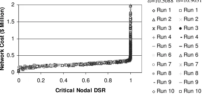
Fig. 3 shows the rate of improvement of the PFMOEA for both solutions obtained. The overall performances of the PFMOEA were rather similar for both ω_=10.5088

and ω_{=10.9031 cases. Though the former began with an initial population of solutions}

with much higher costs, the algorithm progressed rapidly within the first six generations and still succeeded in locating the optimal solution within an impressively low function evaluations count. Fig. 4 shows the pareto-optimal fronts generated for the two ω _{values (for the 10 random runs). All the fronts are virtually the same}

suggesting that the PFMOEA is robust and exhibits a consistent performance.

(Fig. 3 here)

(Fig. 4 here)

5.2 Hanoi network

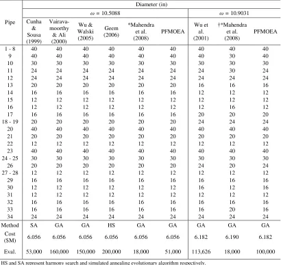
The Hanoi network (Fig. 2b) consists of 34 pipes, 32 nodes and a single source of elevation 100m. The minimum head at all demand nodes is fixed at 30m. A set of six commercially available pipe diameters (12, 16, 20, 24, 30 and 40 in.) is utilised in the design optimization of the system with the cost of each pipe calculated based on the cost function Ci=1.1×Li×Di1.5, where C ($), L (m) and D (in.) are the cost, length and diameter of commercial pipe i respectively. All new pipes are assumed to have a HW roughness coefficient of 130. The network input data can be found in Fujiwara and Khang (1990).

Solutions achieved by other researchers are presented in Table 2. Cunha and Sousa (1999) identified the solution of $6.056 million for ω_{=10.5088 while Wu et al. (2001)}

reported the solution with capital cost of $6.182 million for ω_{=10.9031. These}

which involve the entire solution space) within the lowest numbers of function evaluations in the literature hitherto. Mahendra et al. (2008) achieved the solutions of $6.056 million (ω_{=10.5088) and $6.190 million (}ω_{=10.9031) both within a low}

function evaluation of 18,000. However, it is essential to highlight that a search space reduction technique was implemented and only selective candidate pipe diameters (from the 6 commercial pipe sizes) were used. Hence, the GA search only involved 2.351×1019 possible solutions which is approximately 8.2×10-6 % of the entire solution space (i.e. 634 = 2.865×1026). Also, it includes multiple GA-enhancing techniques and is best suited to systems with a single demand pattern.

For this network, 60 runs each starting from a different initial population (randomly generated) were conducted for each ω _{value. A total of 200,000 function evaluations}

were permitted per run. The crossover probability was fixed to 1.0 and the range of mutation probability used was between 0.005 and 0.02. The PFMOEA succeeded in identifying the least cost feasible solutions for both ω _{values with 51,000 function}

evaluations for the solution of $6.056 million (for ω_{=10.5088) and 100,000 function}

evaluations for the solution of $6.182 million (for ω_{=10.9031) which respectively are}

equivalent to 1.78×10-20 % and 3.49×10-20 % of the entire search space. These values are lower than what was achieved by Mahendra et al. (2008), i.e. 7.656×10-14 % of the reduced solution space. Compared to the 53,000 function evaluations by Cunha and Sousa (1999) and 113,626 function evaluations by Wu et al. (2001), this represents an approximate improvement of 3.77% and 12% for ω_{=10.5088 and} ω_=10.9031

respectively. It is worth mentioning that the PFMOEA also obtained the solution of $6.19021 million which is a similar design to the $6.190 million solution by Mahendra et al. (2008) (all pipe diameters are identical to Mahendra et al. (2008) except for pipe 27 which is 16in) with 49,700 function evaluations.

(Table 2 here)

The least cost solutions presented by Mahendra et al. (2008) and the PFMOEA were simulated using both EPANET-PDX and EPANET 2 to confirm the nodal pressure heads. Pressure heads for the four most critical nodes are presented in Table 3. For the solution with ω_{=10.9031 by Mahendra et al. (2008), it was observed (Table 3) that the}

head at node 27 violates the minimum nodal pressure requirement. All optimum solutions identified by PFMOEA were feasible in that all nodal heads (generated by EPANET-PDX and EPANET 2) were above the minimum pressure requirement.

(Table 3 here)

Table 4 shows the least cost solutions of the six best PFMOEA runs for each of the two ω _{values used here. The critical nodal pressure heads presented confirm that all}

solutions meet the minimum required pressure and are fully feasible. The PFMOEA succeeded in locating the optimal solution four times both for ω_{=10.5088 and} ω_{=10.9031. The costs of the other solutions obtained (as shown in Table 4) were only}

This along with the low number of function evaluations (Table 4) demonstrates that the PFMOEA is highly capable of locating near optimal solutions very quickly.

(Table 4 here)

5.3 New York Tunnels

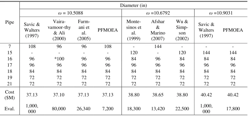
Fig. 2c shows the layout of the New York tunnels. The network is fed from a single fixed-head source providing a head of 91.44m (300 ft) and consists of 20 demand nodes and 21 pipes the details of which can be found in Murphy et al. (1993). The objective of this optimization problem is to expand the existing tunnels by means of pipe paralleling so that the projected demands and pressure requirements can be met. The minimum head constraints are 79.248 m (260 ft) for node 16, 83.149 m (272 ft) for node 17 and 77.724 m (255 ft) for the remaining 18 nodes. There are 15 available diameters to be considered and the “do nothing” option, forming a total solution space of 1621=1.93×1025 possible network designs.

The best solutions reported in the literature by other authors using GA with various constraint handling methods are presented in Table 5. Vairavamoorthy and Ali (2000) reported a solution with a low cost of $37.10 million. However, the pipe diameter of 100in. used in this solution is not in the set of commercial pipe sizes allocated for this optimization problem. Savic and Walters (1997) reported the least cost solutions in the literature hitherto, i.e. $37.13 million for ω_{=10.5088 and $40.42 million for} ω_{=10.9031. The solution of $37.13 million was also identified by Farmani et al.}

(2005) within the lowest reported number of function evaluations so far. To the knowledge of the authors, besides Savic and Walters (1997), no other previous studies in the literature reported solutions using ω_=10.9031.

(Table 5 here)

The solution space of the New York Tunnels problem is approximately one order of magnitude smaller than that of the Hanoi network. Hence, only 30 runs were conducted for each ω _{value. A total of 100,000 function evaluations were permitted}

per run. The crossover probability was fixed to 1.0 and the mutation probability used was between 0.005 and 0.01. For this example, the PFMOEA succeeded in locating the optimal solutions (identical to that of Savic and Walters (1997)) but with remarkably fewer function evaluations in comparison to the rest of the algorithms presented, i.e. 7,200 for ω_{=10.5088 and 17,800 for} ω _{=10.9031. These respectively}

represent extremely small fractions of 3.73×10-22 % and 9.22×10-22 % of the total number of pipe size combinations (1621). In comparison to the algorithms with the smallest numbers of function evaluations, the computational effort (function evaluations) required by the PFMOEA was only 27.33% of that required by Farmani et al. (2005) for ω_{=10.5088 and 1.78% of that required by Savic and Walters (1997)}

It is also worth highlighting that within the 30 random runs executed the optimum solution of $37.13 million was located twice for ω_{=10.5088; the second time within}

8,200 function evaluations which is also much smaller than the 26,340 function evaluations by Farmani et al. (2005). Both optimal solutions obtained by the PFMOEA were simulated by EPANET-PDX and EPANET 2 to reconfirm their feasibility. Results (critical node pressure heads) are presented in imperial units to enable an easy comparison. It can be concluded from Table 6 that all nodal pressure heads meet the minimum pressure requirement.

(Table 6 here)

Table 7 shows the cost of five best feasible solutions generated from the best PFMOEA run for this network for ω_{=10.5088 and} ω_{=10.9031. The costs of these}

solutions were very close to the least cost solutions reported in the literature. This suggests that the PFMOEA is capable of obtaining a Pareto-optimal front consisting of non-dominated solutions which are highly comparable to the best (least cost) solution. A good range of solutions is therefore provided allowing for flexibility in choosing the final design for implementation during a higher level decision making stage which may involve other measures such as reliability.

(Table 7 here)

5.4 Discussion

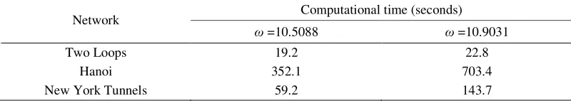
The CPU times required by the PFMOEA to obtain the best reported solutions for all the benchmark networks are presented in Table 8. The PFMOEA was executed using an Intel Core 2 Duo CPU 2.66 GHz personal computer with 3.23 GB RAM.

(Table 8 here)

To further analyse the efficiency and robustness of the approach, the PFMOEA was also formulated with the second objective function being the network DSR to be maximized. Table 9 compares the performance of the PFMOEA with two different 2nd objective functions, i.e. maximizing the critical (i.e. smallest) nodal DSR and maximizing the network DSR. For the latter, the PFMOEA succeeded in locating all the least cost designs in the literature as well but at a much higher computational cost.

(Table 9 here)

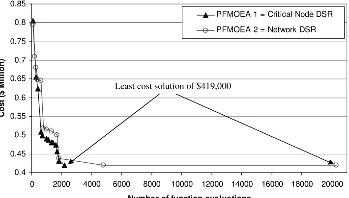
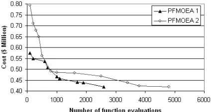
node. The network DSR only represents the average performance of all nodes taken together. Most of the time, the performance of the critical node is overshadowed by other better performing nodes. For example, for a hypothetical network containing 100 nodes, consider a hypothetical solution which is made up of 99 fully satisfied nodes (i.e. DSR = 1) and 1 node with no outflow (i.e. DSR = 0). Though quite infeasible, this solution has an overall network DSR of 0.99 and would be ranked highly in terms of the network DSR. On the other hand, by utilizing the critical node DSR, the worst performing node is perceptibly distinguished amongst other nodes and any solution that has very poor nodal performances will incur a low fitness value. This way the algorithm is better able to identify quickly intermediate solutions that are potentially viable. This distinction (of the worst performing node) may not be particularly significant in the early phase of the evolution process. However, it becomes increasingly vital as solutions evolve through generations (especially near the end of the optimization run) and when the population pool begins to be dense with near-feasible near-optimal solutions. Normally, this is shown by a noticeable plateau in the graph depicting the progress of the algorithm. For example, the progress of the best runs for the Two-loop network (ω _{=10.5088) using both formulations were}

compared in detail as shown in Fig. 5. The PFMOEA based on the critical node DSR formulation will be referred to as PFMOEA 1; the PFMOEA based on the network DSR formulation will be referred to as PFMOEA 2.

(Fig. 5 here)

Both PFMOEA 1 and 2 started off with similar solutions and experienced rapid improvements (reduction in network cost) in the early phase of the evolution. It is worth observing that even at the early evolution stage the progress made by PFMOEA 1 is superior to that of PFMOEA 2. The point which marked the significant difference between formulations began shortly after 1,800 function evaluations where PFMOEA 1 continued to progress and obtained the optimal solution at 2,200 function evaluations while PFMOEA 2 was trapped in a plateau for a further 18,500 function evaluations before locating the optimal solution. The computational effort using the former was only 10.83% of the latter. This clearly shows that the critical node DSR is a better criterion in the decision process as it enforces more pressure on the search to stay close to the boundary as defined by the active constraints where “just feasible” solutions are located, i.e. solutions with low or zero redundancy. The same outcome is observed for both the Hanoi WDS and New York tunnels examples. The progress graphs can be found in Appendix A. Nevertheless, the fact that both PFMOEA formulations succeeded in locating the least cost designs for all networks demonstrates that the approach is highly robust.

evolutionary process. With the accurate performance evaluation of both feasible and infeasible solutions, the active constraint boundaries can be precisely determined with literally no additional computational effort, enabling the feasibility boundary convergent strategy to function effectively.

6 Conclusions

This paper proposes a new penalty-free multi-objective evolutionary optimization approach for WDSs. The described PFMOEA combines a multi-objective evolutionary algorithm with pressure dependent analysis (PDA). PDA is capable of simulating infeasible solutions accurately, providing the means to quickly and accurately identify the feasible region of the solution space without the need for penalty functions or other special constraint handling techniques. The algorithm has been applied to three benchmark networks and the results have been compared in detail with those obtained using other constraint handling algorithms from the literature. For the sample networks, it is demonstrated that the algorithm is exceedingly efficient and robust with the capability of finding the least cost solutions reported in the literature with considerably fewer function evaluations.

The computational efficiency of the algorithm is partly due to the accurate performance evaluation of solutions. Infeasible solutions are accurately simulated and this enhances the boundary search techniques applied including the ability to focus the search around the active constraints. The significant advantage of this method over previous methods is that it eliminates the need for ad-hoc penalty functions or additional “boundary search” parameters. Hence there is no need for any parameter fine tuning or trial and error runs. Therefore, conceptually, the proposed formulation is the simplest by far. The initial results presented herein are very promising. More testing is required to assess the computational efficiency more accurately. Ongoing research includes extension of the new approach to tank sizing and location problems and incorporation of operating costs including pumping costs.

Acknowledgements

References

Afshar MH, Marino MA (2007) A parameter-free self-adapting boundary genetic search for pipe network optimization. Comput. Optim. Appl. 37:83-102

Alperovits E, Shamir U (1977) Design of optimal water distribution systems. Water Resource Research 13(6):885-900

Brkic D (2011) Iterative methods for looped network pipeline calculation. Water Resources Management 25(12):2951–2987. DOI 10.1007/s11269-011-9784-3 Brkic D (2012) Discussion of water distribution system analysis: Newton-Raphson

method revisited. J Hydraulic Engineering, ASCE 138: 822-824

Chadwick A, Morfett J, Borthwick M (2004) Hydraulics in Civil and Environmental Engineering. Spon, Abingdon, UK.

Cunha MC, Sousa J (1999) Water distribution network design optimization: simulated annealing approach. J. Water Resour. Plann. Manage. Div., Am. Soc. Civ. Eng. 125(4): 215-221

Deb K (2000) An efficient constraint handling method for genetic algorithms. Computer Methods in Applied Mechanics and Engineering 186(2):311-338 Deb K, Pratap A, Agarwal S, Meyarivan T (2002) A fast and elitist multiobjective

genetic algorithm: NSGA-II. Evolutionary Computation, IEEE Trans 6(2):182-197

Ekinci O, Konak H (2009) An optimization strategy for water distribution networks. Water Resources Management 23:169-185

Eusuff MM, Lansey KE (2003) Optimization of water distribution network design using the shuffled frog leaping algorithm. Journal of Water Resources Planning and Management, ASCE 129(3):210-225

Farmani R, Wright JA, Savic DA, Walters GA (2005) Self-adaptive fitness formulation for evolutionary constrained optimization of water systems. Journal of Computing in Civil Engineering, ASCE 19(2):212-216

Fujiwara O, Khang DB (1990) A two-phase decomposition method for optimal design of looped water distribution networks. Water Resour. Res. 26(4):539-549

Geem ZW (2006) Optimal cost design of water distribution networks usingharmony search. Engineering Optimization 38(3):259-280

Keedwell E, Khu ST (2006) A novel evolutionary metaheuristic for the multi-objective optimization of real-world water distribution networks. Engineering Optimization, 38(3):319-333

Khu ST, Keedwell E (2005) Introducing choices (flexibility) in upgrading of water distribution network: the new york city tunnel network example. Engineering Optimization, 37(3):291-305

Kumar SM, Narasimhan S, Bhallamudi SM (2010) Parameter estimation in water distribution networks. Water Resources Management 24:1251-1272

Lansey KE, Mays LW (1989) Optimization model for design of water distribution systems. Reliability analysis of water distribution system, L. R. Mays, ed., ASCE, Reston, Va

Mahendra KS, Gupta R, Bhave PR (2008) Optimal design of water networks using genetic algorithm with reduction in search space. J. Water Resour. Plann. Mngmnt, ASCE 134(2):147-160

Murphy LJ, Simpson AR, Dandy GC (1993) Pipe network optimization using an improved genetic algorithm. Res. Rep. No. R109, Dept. Of Ci. and Envr. Eng., Univ. Of Adelaide, Australia

Prasad TD, Park NS (2004) Multiobjective genetic algorithms for design of water distribution networks. J. Hydr. Engrg., ASCE 130(1):73-82

Rossman LA (2002) EPANET 2 User’s Manual, Water Supply and Water Resources Division, National Risk Management Research Laboratory, Cincinnati, OH45268 Savic DA, Walters GA (1997) Genetic algorithms for least-cost design of water

distribution networks. J. Water Resour. Plann. Manage., ASCE 123(2):67-77 Siew C, Tanyimboh TT (2010) Pressure-dependent EPANET extension: extended

period simulation. Proceedings of the 12th Annual Water Distribution Systems Analysis Conference, September 12-15, Tucson, Arizona

Siew C, Tanyimboh TT (2011) The computational efficiency of EPANET-PDX. Proceedings of the 13th Annual Water Distribution Systems Analysis Conference, WDSA 2011, May 22-26, Palm Springs, California

Siew C, Tanyimboh TT (2012) Pressure dependent EPANET extension. Water Resources Management 26(6): 1447-1498

Spiliotis M, Tsakiris G (2011) Water distribution system analysis: Newton-Raphson method revisited. J. Hydraulic Engineering, ASCE 137(8):852-855

Spiliotis M, Tsakiris G (2012a) Closure of water distribution system analysis: Newton-Raphson method revisited. J Hydraulic Engineering, ASCE 138: 824-826 Spiliotis M, Tsakiris G (2012b) Water distribution network analysis under fuzzy

demands. Civil Engineering and Environmental Systems 29(2): 107-122

Su YC, Mays LW, Duan N, Lansey KE (1987) Reliability-based optimization model for water distribution systems. J. Hydr. Engrg., ASCE 114(12):1539-1556

Tanyimboh TT, Burd R, Burrows R, Tabesh M (1999) Modelling and reliability analysis of water distribution systems. Water Science and Technology, IWA 39(4): 249-255

Tanyimboh TT, Templeman AB (2010) Seamless pressure-deficient water distribution system model. J. Water Management, ICE 163(8):389-396

Todini E, Pilati S (1988) A gradient algorithm for the analysis of pipe networks. In: Coulbeck B, Orr C-H (eds) Computer applications in water supply, vol 1. Research Studies Press, England

Vairavamoorthy K, Ali M (2000) Optimal design of water distribution systems using genetic algorithms. Computer-aided Civil and Infrastructure Engineering 15:374-382

Vairavamoorthy K, Ali M (2005) Pipe index vector: a method to improve genetic-algorithm-based pipe optimization. J. Hydr. Engrg., ASCE 131(12):1117-1125 Wu ZY, Boulos PF, Orr CH., Ro JJ (2001) Using genetic algorithm to rehabilitate

distribution systems. Journal American Water Works Association 93(11):74-85 Wu ZY, Simpson AR (2002) A self-adaptive boundary search genetic algorithm and

its application to water distribution systems. J. Hydraul. Res. 40:191-203

Wu ZY, Walski T (2005) Self-adaptive penalty approach compared with other constraint-handling techniques for pipeline optimization. J. Water Resour. Plann. Manage., ASCE 131(3):181-192

Figures

Boundary region

Fig. 1a Pareto optimal front with boundary search

Fig. 1b Pareto optimal front without boundary search

Fig. 2b Layout of Hanoi network

0.4 0.5 0.6 0.7 0.8 0.9

0 2 4 6 8 10 12 14 16 18 20 22 24 26

Generation C o s t ($ M il li o n ) =10.5088 =10.9031 ω ω

Fig. 3 Progress of PFMOEA for the Two-Loop network

Fig. 4 Pareto-optimal fronts for the Two-loop network

0 0.5 1 1.5 2

0 0.2 0.4 0.6 0.8 1

Critical Nodal DSR

N e tw o rk C o s t ($ M il li o n

) _{Run 1 Run 1}

Run 2 Run 2

Run 3 Run 3

Run 4 Run 4

Run 5 Run 5

Run 6 Run 6

Run 7 Run 7

Run 8 Run 8

Run 9 Run 9

Run 10 Run 10

Fig. 5 Progress of the PFMOEA using different formulations for the Two Loop Network

0.4 0.45 0.5 0.55 0.6 0.65 0.7 0.75 0.8 0.85

0 2000 4000 6000 8000 10000 12000 14000 16000 18000 20000

Number of function evaluations

C

o

s

t

($

M

il

li

o

n

)

PFMOEA 1 = Critical Node DSR

PFMOEA 2 = Network DSR

Tables

Table 1 Solutions of the Two-Loop network

Diameter (in)

ω _{= 10.5088} ω _{= 10.9031}

Pipe _{Savic &}

Walters (1997)

Cunha & Sousa (1999)

Wu et al. (2001)

Eusuff & Lansey (2003)

PFMOEA

Savic & Walters (1997)

PFMOEA

1 18 18 18 18 18 20 20

2 10 10 10 10 10 10 10

3 16 16 16 16 16 16 16

4 4 4 4 4 4 1 1

5 16 16 16 16 16 14 14

6 10 10 10 10 10 10 10

7 10 10 10 10 10 10 10

8 1 1 1 1 1 1 1

Method GA SA GA SFLA GA GA GA

Cost ($) 419,000 419,000 419,000 419,000 419,000 420,000 420,000

Eval. 250,000 25,000 7,467 11,323 2,200 250,000 2,600

SA represents simulated annealing.

Table 2 Solutions of the Hanoi Network

Diameter (in)

ω _{= 10.5088} ω _{= 10.9031}

Pipe Cunha & Sousa (1999)

Vairava- moorthy & Ali (2000)

Wu & Walski (2005)

Geem (2006)

*Mahendra et al. (2008)

PFMOEA

Wu et al. (2001)

†*Mahendra et al. (2008)

PFMOEA

1 - 8 40 40 40 40 40 40 40 40 40

9 40 40 40 40 40 40 40 30 40

10 30 30 30 30 30 30 30 30 30

11 24 24 24 24 24 24 24 30 24

12 24 24 24 24 24 24 24 24 24

13 20 20 20 20 20 20 16 16 16

14 16 16 16 16 16 16 12 12 12

15 12 12 12 12 12 12 12 12 12

16 12 12 12 12 12 12 12 16 12

17 16 16 16 16 16 16 20 20 20

18 - 19 20 20 20 20 20 20 24 24 24

20 40 40 40 40 40 40 40 40 40

21 20 20 20 20 20 20 20 20 20

22 12 12 12 12 12 12 12 12 12

23 40 40 40 40 40 40 40 40 40

24 - 25 30 30 30 30 30 30 30 30 30

26 20 20 20 20 20 20 24 20 24

27 - 28 12 12 12 12 12 12 12 12 12

29 16 16 16 16 16 16 16 16 16

30 12 12 12 12 12 12 16 12 16

31 12 12 12 12 12 12 12 12 12

32 16 16 16 16 16 16 16 16 16

33 16 16 16 16 16 16 16 20 16

34 24 24 24 24 24 24 24 24 24

Method SA GA GA HS GA GA GA GA GA

Cost

($M) 6.056 6.056 6.056 6.056 6.056 6.056 6.182 6.190 6.182 Eval. 53,000 160,000 150,000 200,000 18,000 51,000 113,626 18,000 100,000

HS and SA represent harmony search and simulated annealing evolutionary algorithm respectively. * Selective diameters used (not the full set of 6 commercial pipe sizes).

Table 3 Critical Node Pressure Heads for the Hanoi Network

Cost ($ Million) 6.056 6.190 6.19021 6.182

ω 10.5088 10.9031

Approach

PFMOEA and Mahendra et al.

(2008)

Mahendra

et al. (2008) PFMOEA

Nodes Heads (m)

27 30.207

(30.170) *29.984 (29.944) 30.331 (30.291) 30.413 (30.377)

29 30.260

(30.220) 30.186 (30.146) 30.088 (30.046) 30.681 (30.646)

30 30.521

(30.483) 30.703 (30.664) 30.596 (30.556) 30.225 (30.188)

31 30.802

(30.764) 31.019 (30.981) 30.912 (30.872) 30.376 (30.339)

* Infeasible solution i.e. Hni < 30 m

Critical node heads generated by EPANET 2 are shown in parentheses

Table 4 Solutions from the Best Six PFMOEA Runs for the Hanoi Network

ω =10.5088 ω =10.9031

Best

Runs Costs

($ Million) Function Evaluations Critical Nodal Heads (m) Costs ($ Million) Function Evaluations Critical Nodal Heads (m)

1 6.056 51,000 30.207 6.182 100,000 30.225

2 6.056 75,400 30.207 6.182 100,100 30.225

3 6.056 87,000 30.207 6.182 111,400 30.225

4 6.056 167,400 30.207 6.182 136,700 30.225

5 6.064 69,900 30.156 6.187 78,600 30.018

6 6.072 46,200 30.271 6.19021 49,700 30.046

Table 5 Solutions of the New York Tunnels

Diameter (in)

ω = 10.5088 ω =10.6792 ω =10.9031

Pipe _{Savic &} Walters (1997) Vaira-vamoor-thy & Ali (2000) Farm-ani et al. (2005) PFMOEA Monte-sinos et al. (1999) Afshar & Marino (2007) Wu & Simp-son (2002) Savic & Walters (1997) PFMOEA

7 108 96 96 108 - 144 - - -

15 - - - - 120 - 120 144 144

16 96 *100 96 96 84 96 84 84 84

17 96 96 96 96 96 96 96 96 96

18 84 84 84 84 84 84 84 84 84

19 72 72 72 72 72 72 72 72 72

21 72 72 72 72 72 72 72 72 72

Cost

($M) 37.13 37.10 37.13 37.13 38.80 38.65 38.80 40.42 40.42

Eval. 1,000,

000 80,000 26,340 7,200 18,300 13,420 22,500

1,000,

000 17,800

* Pipe diameter 100in is not in the set of commercial pipe sizes allocated in this optimization problem

Table 6 Critical Node Pressure Heads for the New York Tunnels

ω _{= 10.5088} ω _{= 10.9031}

Node

Minimum Required

Head (ft) EPANET Head _(ft) EPANET-PDX _{Head (ft)} EPANET Head _(ft) EPANET-PDX _{Head (ft)}

16 260.0 260.161 260.212 260.282 260.332

17 272.8 272.861 272.89 272.882 272.912

19 255.0 255.206 255.266 255.398 255.458

Table 7 Solutions from the best PFMOEA Run for the New York Tunnels

ω _=10.5088 ω _=10.9031

Solution _Cost

($ Million)

Critical Node

Head

(m) _{($ Million)} Cost Critical _Node Head _(m)

1 37.13* 17 83.1769 40.42* 17 83.1836

2 37.62 17 83.2101 41.12 17 83.1866

3 38.13 17 83.2391 41.13 17 83.1896

4 38.80 17 83.2412 41.29 17 83.2719

5 38.94 16 79.3455 41.96 17 83.2750

* Least cost solution reported in the literature. Required head for node 17 is 83.149m. Required Head for node 16 is 79.248m.

Table 8 Computational time required by the PFMOEA to obtain the best reported solutions

Computational time (seconds) Network

ω _=10.5088 ω _=10.9031

Two Loops 19.2 22.8

Hanoi 352.1 703.4

New York Tunnels 59.2 143.7

Table 9 Performance of the PFMOEA with different 2nd objective functions

Number of Function Evaluations

Network ω Cost ($) _{Maximise critical nodal}

DSR Maximize network DSR

10.5088 4.190×105 _{2,200 20,300}

Two Loops

10.9031 4.200×105 2,600 4,800

10.5088 6.056×106 51,000 258,200

Hanoi

10.9031 6.182×106 100,000 336,300

10.5088 37.13×106 7,200 554,400

New York

Appendix A

Fig. 6 Comparison of the evolutionary rate of cost improvement for the critical-node and network-wide DSR formulations

Progress of PFMOEA for Hanoi network (ω _{= 10.5088)}

Progress of PFMOEA for Hanoi network (ω _{= 10.9031)}

Progress of PFMOEA for New York tunnels (ω _{= 10.5088)}

Progress of PFMOEA for New York tunnels (ω _{= 10.9031)}

Progress of PFMOEA for Two Loop network (ω _{= 10.5088)}

List of Tables

Table 1 Solutions of the Two-Loop network Table 2 Solutions of the Hanoi Network

Table 3 Critical Node Pressure Heads for the Hanoi Network

Table 4 Solutions from the Best Six PFMOEA Runs for the Hanoi Network Table 5 Solutions of the New York Tunnels

Table 6 Critical Node Pressure Heads for the New York Tunnels

Table 7 Solutions from the best PFMOEA Run for the New York Tunnels

Table 8 Computational time required by the PFMOEA to obtain the best reported solutions

List of Figures

Fig. 1a Pareto optimal front with boundary search Fig. 1b Pareto optimal front without boundary search Fig. 2a Layout of Two-Loop network

Fig. 2b Layout of Hanoi network Fig. 2c Layout of New York Tunnels

Fig. 3 Progress of PFMOEA for the Two-Loop network Fig. 4 Pareto-optimal fronts for the Two-loop network

Fig. 5 Progress of the PFMOEA using different formulations for the Two Loop Network