Parallelizing Big Data Machine Learning
Applications with Model Rotation
Bingjing ZHANG, Bo PENG and Judy QIU
School of Informatics and Computing, Indiana University, Bloomington, IN, USA
Abstract.This paper proposes model rotation as a general approach to parallelize big data machine learning applications. To solve the big model problem in paral-lelization, we distribute the model parameters to inter-node workers and rotate dif-ferent model parts in a ring topology. The advantage of model rotation comes from maximizing the effect of parallel model updates for algorithm convergence while minimizing the overhead of communication. We formulate a solution using com-putation models, programming interfaces, and system implementations as design principles and derive a machine learning framework with three algorithms built on top of it: Latent Dirichlet Allocation using Collapsed Gibbs Sampling, Matrix Factorization using Stochastic Gradient Descent and Cyclic Coordinate Descent. The performance results on an Intel Haswell cluster with max 60 nodes show that our solution achieves faster model convergence speed and higher scalability than previous work by others.
Keywords.machine learning, big data, big model, parallelization, model rotation
1. Introduction
Machine learning applications such as Latent Dirichlet Allocation (LDA) and Matrix Factorization (MF) have been successfully applied on big data within various domains. For example, Tencent uses LDA for search engines and online advertising [1] while Facebook1uses MF to recommend items to more than one billion people. With tens of billions of data entries and billions of model parameters, these applications can help data scientists to gain a better understanding of big data.
However, the growth of data size and model size makes it hard to deploy these machine learning applications in a way that scales to our needs. A huge amount of effort has been invested in parallelization of these applications, and yet much of the literature deals with a framework-based approach using tools such as MPI2, (Iterative) MapReduce [2][3], Graph/BSP [4], and Parameter Server [5]. At this stage, it remains unclear what is the best approach to parallelization.
To bridge the gap, we propose a systematic approach, “model rotation”, which im-proves the efficiency of model convergence speed and provides high scalability. This solution involves fine-grained synchronization mechanisms in handling parallel model
1
https://code.facebook.com/posts/861999383875667/recommending-items-to-more-tha n-a-billion-people
updates. In the context of this paper, “model rotation” is a generalized parallel computa-tion model that performs parallel model parameter computacomputa-tion via rotacomputa-tion of different model parts in a ring topology. We provide programming interfaces for model rotation in Harp MapCollective framework [6]. Further optimizations include pipelining to reduce the communication overhead and dynamically controlling the time point of the model rotation.
We investigate three core algorithms: Collapsed Gibbs Sampling (CGS) for LDA [7], Stochastic Gradient Descent (SGD) for MF [8] and Cyclic Coordinate Descent (CCD) for MF [9]. The experiments run with different datasets on up to a maximum of 60 nodes and 1200 threads in an Intel Haswell cluster. We compare our CGS, SGD and CCD im-plementations under model rotation-based framework with state-of-the-art implementa-tions (Petuum for CGS, NOMAD for SGD and CCD++ for CCD) running side-by-side on the same cluster. The results show that our solution exceeds their model convergence speeds.
The rest of this paper is organized as follows. Section 2 explores the features of model update in machine learning algorithms and the advantages of model rotation. Sec-tion 3 describes the programming interface and the implementaSec-tion. The experiment re-sults are shown in Section 4, while Section 5 describes the related work. Section 6 gives the conclusion.
2. Algorithms and Computation Models
In this section, we observe three important features of model updates in machine learning algorithms (CGS for LDA, SGD and CCD for MF) whose model update formula is not of the summation form introduced in [10]. For the algorithm parallelization, by discussing the efficiency of different computation models, we highlight the benefits of using model rotation.
2.1. Algorithms
Many machine learning algorithms are built on iterative computation, which can be for-mulated as
At=F(D,At−1) (1)
In this equation,Dis the observed dataset,Ais model parameters to learn, andF is the model update function. The algorithm keeps updating modelA until convergence (by reaching a stop criterion or a fixed number of iterations).
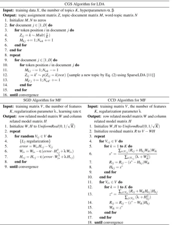
We use CGS for LDA, and SGD or CCD for MF as examples to show the nature of model update dependency. The sequential pseudo code of the three algorithms is listed in Table 1. LDA is a generative modeling technique using latent topics. CGS algorithm learns the model parameters by going through the tokens in a collection of documents
Dand computing the topic assignmentZi j on each tokenXi j=wby sampling from a
multinomial distribution of a conditional probability ofZi j:
p Zi j=k|Z¬i j,Xi j,α,β
∝ N
¬i j wk +β
∑wN
¬i j wk +Vβ
Mk j¬i j+α
Table 1. Sequential Pseudo Code of Machine Learning Algorithm Examples
CGS Algorithm for LDA Input:training dataX, the number of topicsK, hyperparametersα,β
Output: topic assignment matrixZ, topic-document matrixM, word-topic matrixN
1. InitializeM,Nto zeros 2. fordocumentj∈[1,D]do
3. fortoken positioniin documentjdo 4. Zi j=k∼Mult(K1)
5. Mk j+=1;Nwk+=1 6. end for
7. end for 8. repeat
9. fordocumentj∈[1,D]do
10. fortoken positioniin documentjdo 11. Mk j−=1;Nwk−=1
12. Zi j=k0∼p(Zi j=k|rest){sample a new topic by Eq. (2) using SparseLDA [11]} 13. Mk0j+=1;Nwk0+=1
14. end for 15. end for 16. untilconvergence
SGD Algorithm for MF CCD Algorithm for MF
Input:training matrixV, the number of features
K, regularization parameterλ, learning rateε
Output: row related model matrixWand column related model matrixH
1. InitializeW,HtoUniformReal(0,1/√K)
2. repeat
3. for randomVi j∈Vdo 4. {L2regularization} 5. error=Wi∗H∗j−Vi j
6. Wi∗=Wi∗−ε(error·H∗j|+λWi∗) 7. H∗j=H∗j−ε(error·Wi∗|+λH∗j) 8. end for
9. untilconvergence
Input: training matrixV, the number of features
K, regularization parameterλ
Output: row related model matrixWand column related model matrixH
1. InitializeW,HtoUniformReal(0,1/√K)
2. Initialize residual matrixRtoV−WH
3. repeat
4. forV∗j∈Vdo 5. fork=1toKdo
6. s∗= ∑i∈V∗j(
Ri j+Hk jWik)Wik
∑i∈V∗j(λ+W
2 ik) 7. Ri j=Ri j−(s∗−Hk j)Wik 8. Hk j=s∗
9. end for 10. end for 11. forVi∗∈Vdo 12. fork=1toKdo
13. z∗= ∑j∈Vi∗(Ri j+WikHk j)Hk j ∑j∈Vi∗(λ+H
2 k j) 14. Ri j=Ri j−(z∗−Wik)Hk j 15. Wik=z∗
16. end for 17. end for 18. untilconvergence
In this equation, superscript¬i jmeans that the corresponding token is excluded.Vis the vocabulary size. Nwk is the current token count of the wordwassigned to topickinK
topics, andMk jis the current token count of the topickassigned in the document j.α
andβ are hyperparameters. The model includesZ,N,Mand∑wNwk. WhenXi j=wis
computed, some elements in the related rowNw∗and columnM∗jare updated. Therefore
dependencies exist among different tokens when accessing or updatingNandMmodel matrices.
matrixH(model). SGD algorithm learns the model parameters by optimizing the object loss function composed by a squared error and a regularizer (L2regularization is used here). When an elementVi jis computed, the related row vectorWi∗and column vector H∗j are updated. The gradient calculation of the next random elementVi0j0 depends on
the previous updates inWi0∗andH∗j0. CCD also solves MF application. But unlike SGD, the model update order firstly goes through all the rows inWand then the columns inH, or all the columns inHfirst and then rows inW. The model update inside each row ofW
or column ofHgoes through feature by feature.
Parallelization of these iterative algorithms can be done by utilizing either the paral-lelism inside different components of model update functionFor the parallelism among multiple invocations ofF. For the first category, the difficulty of parallelization lies in the computation dependencies insideF, which are either between the data and the model or among the model parameters. IfFis in a “summation form”, such algorithms can be easily parallelized through the first category [10]. However, in large-scale learning ap-plications, the algorithms picking random examples in model update perform asymptot-ically better than the algorithms with the summation form [12]. In this paper, we focus on this type of algorithm with the second category of parallelism where the difficulty of parallelization lies in the dependencies between iterative updates of a model parameter. Thus when the dataset is partitioned toPparts, model updates in this kind of algorithm only use one part of data entriesDpas
At=F(Dp,At−1) (3)
Obtaining the exactAt−1is not feasible in parallelization. It is challenging to parallelize different invocations ofF. However, these algorithms have certain features which can maintain the algorithm correctness and improve the parallel performance.
I.The algorithms can converge even when the consistency of a model is not guar-anteed to some extent.Algorithms can work on modelAwith an older versioniwheni
is within bounds [13], as shown in
At=F(Dp,At−i) (4)
By using a different version ofA, Feature I breaks the dependency across iterations.
II.The update order of the model parameters is exchangeable.Although different update orders can lead to different convergence rates, they normally don’t make the al-gorithm diverge. IfFonly accesses and updates one of the disjointed parts of the model parameters (Ap0), there is a chance of finding an arrangement on the order of model up-dates that allows independent model parts to be processed in parallel while keeping the dependencies.
Atp0 =F(Dp,At−1
p0 ) (5)
In CGS, we provide one update order by document, but other orders such as updating by words are also correct since CGS allows order exchange. Two tokens of different words in different documents can be trained in parallel since there is no update conflict in model matricesNandM.
model parameters for updating is done through randomly selecting examples from the dataset. In CCD, the selection of rows or columns is also random.
2.2. Computation Models
A detailed description of computation models can be found in previous work [15]. Our summary of related work helps to define computation models based on two properties. One is whether the computation model uses synchronous or asynchronous algorithms for parallelization. Another looks at whether the model parameters used in computation are the latest or stale. Both the synchronization strategies and the model consistency can impact model convergence speed.
Computation models using stale model parameters can be easily applied based on Feature I of model updates. However, it does come with certain performance issues such as less effective model updates. When a synchronized algorithm is applied, the compu-tation model can be implemented via “allreduce”. By doing so, the routing can be opti-mized while each worker retains a full copy of the model. For big models, this causes high memory usage and can result in failure to scale for applications. Another method is allowing each worker to only fetch the model parameters related to the local train-ing data. This saves memory but offers less opportunity for routtrain-ing optimization. When an asynchronous algorithm is used, the computation model reduces the synchronization overhead. However, since each worker directly communicates large numbers of model updates, routing among the workers cannot be optimized. Without synchronization barri-ers, this computation model does not aim for complete synchronization of model copies on all the workers. As such, the model convergence speed is affected by the real network speed. To solve this problem, Q. Ho et al. combine asynchronous algorithms and syn-chronized algorithms into one computation model to guarantee the model convergence and improve the speed [13].
The computation model with the latest model parameters provides more effective model updates. It is commonly performed through “model rotation”. This method shows many advantages. Unlike computation models using stale model parameters, there is no additional local copy for model parameters fetched during the synchronization, meaning the memory usage is low. Plus in a distributed environment, the communication only happens between two neighboring workers so that the routing can be easily optimized.
CGS, SGD and CCD can all be implemented by the above-mentioned computation models because of Features I and II of model updates [16][17][18][19][20][21][22]. Al-though model rotation performs better [17][18][19][22], it may result in high synchro-nization overhead in these algorithms due to the dataset being skewed and the unbalanced workload of each worker [23][24]. Therefore the completion of an iteration has to wait for the slowest worker. If the straggler acts up, the cost of synchronization becomes even higher. In the implementation of our model rotation framework, we take these problems into consideration and minimize the overhead.
3. Programming Interface and Implementation
commu-nication operations to synchronize Map tasks. The following demonstrates how model rotation is applied to three algorithms: CGS for LDA, SGD and CCD for MF.
3.1. Data and Model
The structure of the training data can be generalized as a tensor. For example, the dataset in CGS is a document-word matrix. In SGD, the dataset is explicitly expressed as a matrix. When it is applied to recommendation systems, each row of the matrix represents a user and each column an item; thus every element represents the rating of a user to an item. In these matrix structured training data, a row has a row-related model parameter vector as does a column. For quickly visiting data entries and related model parameters, indices are built on the row IDs and column IDs. Based on the model settings, the number of elements per vector can be very large. As a result, both row-related and column-related model structures might be large matrices.
In CGS and SGD, the model update function allows for the data to be split by rows or columns so that one model (with regards to the matching row or column of training data) is cached with the data, leaving the other to be rotated. For CCD, the model update function requires both the row-related model matrixW and the column-related model matrixHto be rotated. We abstract the model for rotation as a distributed data structure organized as partitions and indexed with partition IDs. A partition can be expressed as an array if the vector is dense, or as a key-value pair if sparse. In CGS, each partition holds a word’s topic counts. In SGD, each partition holds a column’s related model parameter vector. In CCD, each partition holds a feature dimension’s parameters of all the rows or columns.
3.2. Operation API
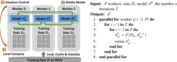
We express model rotation as a collective communication. The operation takes the model part owned by a process and performs the rotation. By default, the operation sends the model partitions to the next neighbor and receives the model partitions from the last neighbor in a predefined ring topology of workers. An advanced option is that we can dy-namically define the ring topology before performing the model rotation. Thus program-ming model rotation requires just one API. For local computation inside each worker, we simply program it through an interface of “schedule-update”. A scheduler employs a user-defined function to maintain a dynamic order of model parameter updates and avoid the update conflict. Since the local computation only needs to process the model obtained during the rotation without considering the parallel model updates from other workers, the code of a parallel machine learning algorithm can be modularized as a process of performing computation and rotating model partitions (see Figure 1).
3.3. Pipelining and Dynamic Rotation Control
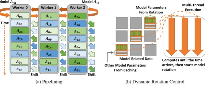
The model rotation operation is implemented as a non-blocking call so that the efficiency of model rotation can be optimized through pipelining. We divide the distributed model parameters on all the workers into two setsA∗aandA∗b(see Figure 2a). The pipelined
model rotation is conducted in the following way: all the workers first compute Model
A∗awith related local data. Then they start to shiftA∗a, and at the same time they
Training Data 𝑫on HDFS
Load, Cache & Initialize 3Iteration Control
Worker 2 Worker 1
Worker 0
Local Compute 1
2Rotate Model
Model 𝑨𝟎𝒕𝒊 Model 𝑨𝟏𝒕𝒊 Model 𝑨𝟐𝒕𝒊
Training
Data 𝑫𝟎 Training Data 𝑫𝟏 Training Data𝑫𝟐
Input: Pworkers, dataD, modelA0, the number of iterationsT
Output: At
1. parallel forworkerp∈[1,P]do 2. fort=1toTdo
3. fori=1toPdo
4. Ati
p0=F(Dp,A ti−1 p0 ) 5. rotateAti
p0
[image:7.595.129.466.156.275.2]6. end for 7. end for 8. end parallel for
Figure 1. Execution Flow and Pseudo Code of Model Rotation
All workers wait for the completion of corresponding model rotations and then begin computing model updates again. Therefore the communication is overlapped with the computation. In this pipelining mechanism, each time a chunk of model parameters is computed and communicated. In experiments, communicating model parameters in large batches is more efficient than flooding the network with small messages [23].
Utilizing Features II and III in model update, we also allow dynamic control on the invocation of model rotation based on the time spent on computation (see Figure 2b). In CGS for LDA and SGD for MF, assuming each worker caches rows of data and row-related model parameters and obtains column-row-related model parameters through rotation, it then selects related training data to perform local computation. We split the data and model into small blocks which the scheduler dynamically selects for model update while avoiding the model update conflicts on the same row or column. Once a block is pro-cessed by a thread, it reports the status back to the scheduler. Then the scheduler searches another free block and dispatches to an idle thread. We set a timer to oversee the training progress. When the designated time arrives, the scheduler stops dispatching new blocks, and the execution ends. Because the computation is load balanced with the same length of time, the synchronization overhead is reduced. In the iterations of model rotations, the time length is further adjusted based on the amount of data items processed. But in CCD, the algorithm dependency does not allow us to dynamically control the model ro-tation. The reason is that in each iteration of CCD, each model parameter is only up-dated once. Using dynamic control results in incomplete model updates in each iteration, which reduces the model convergence speed.
3.4. Algorithm Parallelization
Worker 2 Worker 1
Worker 0
Time
𝑨𝟏𝒂
𝑨𝟎𝒃 𝑨𝟎𝒂
𝑨𝟐𝒃 𝑨𝟐𝒂
𝑨𝟏𝒂 𝑨𝟏𝒃
𝑨𝟏𝒃 𝑨𝟎𝒂
𝑨𝟐𝒂 𝑨𝟐𝒃
𝑨𝟏𝒃 𝑨𝟏𝒂
𝑨𝟎𝒂 𝑨𝟎𝒃
𝑨𝟎𝒃
𝑨𝟐𝒂
𝑨𝟏𝒂 𝑨𝟏𝒃
𝑨𝟎𝒃 𝑨𝟎𝒂
𝑨𝟐𝒂 𝑨𝟐𝒃
𝑨𝟐𝒃
Model 𝑨∗𝒂 Model 𝑨∗𝒃
Shift Shift Shift
(a) Pipelining
Other Model Parameters From Caching
Model Parameters From Rotation
Model Related Data Computes until the time arrives, then starts model rotation
Multi-Thread Execution
[image:8.595.131.466.162.301.2](b) Dynamic Rotation Control
Figure 2. Model Rotation Mechanisms
keep an upper bound and a lower bound for the amount of tokens trained between two invocations of model rotation.
• SGD:BothW andHare model matrices. Assumingn<m, thenV is regrouped by rows,W is partitioned withV, andHis the model for rotation. The ring topol-ogy for rotation is randomized per iteration for accelerating the model conver-gence. For pipelining and load balancing, we estimate the ratio of computation and communication cost, and determine the time point to perform model rotation. • CCD:BothW andHare model matrices. Because model update on a row ofW
needs all the related data items on the same row and model update on a column of
Hneeds all the related data items on the column, the training data is duplicated so that one is regrouped by rows and another is regrouped by columns among work-ers. However, the model update on each feature dimension is still independent. Then we splitW andHby features and distribute them across workers. BothW
andHare rotated for parallel updating of each feature vector inW andH.
4. Experiments
4.1. Training Dataset and Model Parameter Settings
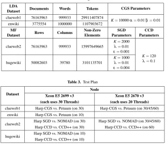
Four datasets are used in the experiments. For LDA and MF applications, each has one small dataset and one big dataset. The datasets and related training parameters are pre-sented in Table 2. Two big datasets are generated from the same source “ClueWeb09”3, while two small datasets are generated from Wikipedia4. With different types of datasets, we show the effectiveness of our model rotation solution on the model convergence speed. In LDA, the model convergence speed is evaluated with respect to the model like-lihood, which is a value calculated from the trained word-topic model matrix. In MF, the model convergence speed is evaluated by the value of Root Mean Square Error (RMSE) calculated on the test dataset, which is from the original matrixV but separated from the
3
Table 2. Training Datasets
LDA
Dataset Documents Words Tokens CGS Parameters
clueweb1 76163963 999933 29911407874
K=10000α=0.01β=0.01 enwiki 3775554 1000000 1107903672
MF
Dataset Rows Columns
Non-Zero Elements
SGD Parameters
CCD Parameters
clueweb2 76163963 999933 15997649665
K=2000
λ=0.01
ε=0.001
K=120
λ=0.1 hugewiki 50082603 39780 3101135701
K=1000
λ=0.01
ε=0.004
Table 3. Test Plan
Dataset
Node
Xeon E5 2699 v3 (each uses 30 Threads)
Xeon E5 2670 v3 (each uses 20 Threads)
clueweb1 Harp CGS vs. Petuum (on 30) Harp CGS vs. Petuum (on 30/45/60) enwiki Harp CGS vs. Petuum (on 10)
clueweb2 Harp SGD vs. NOMAD (on 30) Harp CCD vs. CCD++ (on 30)
Harp SGD vs. NOMAD (on 30/45/60) Harp CCD vs. CCD++ (on 60)
hugewiki Harp SGD vs. NOMAD (on 10) Harp CCD vs. CCD++ (on 10)
training dataset. In addition, we examine the scalability of implementations through the tests on the big datasets.
4.2. Comparison of Implementations
We compare six implementations in the experiments. First is CGS implemented with Harp compared to CGS implemented with Petuum LDA5. Then we compare SGD imple-mented with Harp to SGD impleimple-mented with NOMAD6. Later we compare CCD imple-mented with Harp to CCD++7. The three compared implementations are the fastest open-source implementations we surveyed from the related work. Note that Petuum LDA, NOMAD and CCD++ are all implemented in C++11 while Harp CGS and Harp SGD are implemented in Java 8, so it is quite a challenge for us to exceed them in perfor-mance. Petuum LDA uses Open MPI8for processes, POSIX threads for multi-threading, and ZeroMQ9for communication. Although Petuum uses model rotation at an inter-node level, intra-node multi-threading is deployed with asynchronous algorithms and stale model parameters. NOMAD uses MPICH210for inter-node processes and
In-5 https://github.com/petuum/strads/tree/master/apps/lda_release 6 http://bikestra.github.io
7 http://www.cs.utexas.
edu/~rofuyu/libpmf 8
https://www.open-mpi.org 9
tel Thread Building Blocks11for multi-threading. In NOMAD, MPI Send/MPI Recv are communication operations, but the destination of model shifting is randomly selected without following a ring topology. CCD++ also uses MPICH2 for inter-node processes with collective communication operations and OpenMP12for multi-threading.
4.3. Parallel Execution Environment
Experiments are conducted on a 128-node Intel Haswell cluster at Indiana University. Among them, 32 nodes each have two 18-core Xeon E5-2699 v3 processors (36 cores in total), and 96 nodes each have two 12-core Xeon E5-2670 v3 processors (24 cores in total). All the nodes have 128 GB memory and are connected by QDR InfiniBand. For our tests, JVM memory is set to “-Xmx120000m -Xms120000m”, and IPoIB is used for communication. The implementations are tested on two types of machines separately (see Table 3). We focus on the convergence speed and scaling on the test configurations in which computation time is still the main part of the whole execution. For the small datasets, we use 10 Xeon E5-2699 v3 nodes each with 30 threads, while the big datasets are undertaken by 30 Xeon E5-2699 v3 nodes each with 30 threads and 60 Xeon E5-2670 nodes each with 20 threads to compare the model convergence speed among different implementations. We further examine the scalability with 30, 45, and 60 Xeon E5-2670 v3 nodes each with 20 threads.
4.4. Model Convergence Speed
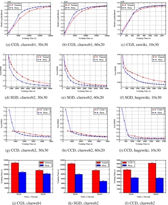
In CGS, through examination of the model likelihood achieved by the training time, the results on two different datasets all show that Harp consistently outperforms Petuum. We test Harp CGS and Petuum on “clueweb1” with 30×30 and 60×20 two configurations (see Figure 3a and Figure 3b). Both results show that Harp CGS converges faster than Petuum. We also test “enwiki” on 10×30 and the result is the same (see Figure 3c). Concerning the convergence speed on the same dataset with different configurations, we observe that the fewer the number of cores used and the more computation per core, the faster Harp runs compared to Petuum. When the scale goes up, the difference in the convergence speed reduces. With 30×30 Xeon E5-2699 v3 nodes, Harp is 45% faster than Petuum while with 60×20 Xeon E5-2670 v3 nodes, Harp is 18% faster than Petuum when the model likelihood converges to−1.37×10¹¹(see Figure 3j).
In SGD, Harp SGD also converges faster than NOMAD. On “clueweb2” (see Figure 3d and Figure 3e), with 30×30 Xeon E5-2699 v3 nodes, Harp is 58% faster, and with 60×20 Xeon E5-2670 v3 nodes, Harp is 93% faster when the test RMSE value converges to 1.61 (see Figure 3k). The difference in the convergence speed increases because the random shifting mechanism in NOMAD becomes unstable when the scale goes up. We also test the small dataset “hugewiki” on 10×30 Xeon E5-2699 v3 nodes, and the result remains that Harp SGD is faster than NOMAD (see Figure 3f).
In CCD, we again test the model convergence speed on “clueweb2” and “hugewiki” datasets (see Figure 3g, Figure 3h and Figure 3i). The results show that Harp CCD also has comparable performance with CCD++. Note that CCD++ uses a different model update order, so that the convergence rate based on the same number of model update
11
0 5000 10000 15000 20000 Training Time (s) 3.0 2.8 2.6 2.4 2.2 2.0 1.8 1.6 1.4 1.2 Model Log-likelihood 1e11 Petuum Harp
(a) CGS, clueweb1, 30x30
0 5000 10000 15000 20000 Training Time (s) 3.0 2.8 2.6 2.4 2.2 2.0 1.8 1.6 1.4 1.2 Model Log-likelihood 1e11 Petuum Harp
(b) CGS, clueweb1, 60x20
0 200 400 600 800 1000 1200 1400 Training Time (s) 1.2 1.1 1.0 0.9 0.8 0.7 0.6 0.5 Model Log-likelihood 1e10 Petuum Harp
(c) CGS, enwiki, 10x30
0 1000 2000 3000 4000 5000 6000 7000 8000 Training Time (s)
1.6 1.7 1.8 1.9 2.0 2.1 2.2 Test RMSE Nomad Harp
(d) SGD, clueweb2, 30x30
0 1000 2000 3000 4000 5000 6000 7000 8000 Training Time (s)
1.6 1.7 1.8 1.9 2.0 2.1 2.2 Test RMSE Nomad Harp
(e) SGD, clueweb2, 60x20
0 500 1000 1500 2000 2500 3000 3500 4000 Training Time (s) 0.50 0.55 0.60 0.65 Test RMSE Nomad Harp
(f) SGD, hugewiki, 10x30
0 1000 2000 3000 4000 5000 Training Time (s) 1.6 1.7 1.8 1.9 2.0 2.1 2.2 2.3 2.4 Test RMSE CCD++ Harp
(g) CCD, clueweb2, 30x30
0 1000 2000 3000 4000 5000 Training Time (s)
1.6 1.7 1.8 1.9 2.0 2.1 2.2 2.3 2.4 Test RMSE CCD++ Harp
(h) CCD, clueweb2, 60x20
0 500 1000 1500 2000 2500 3000 3500 Training Time (s) 0.5 0.6 0.7 0.8 0.9 1.0 1.1 1.2 1.3 1.4 Test RMSE CCD++ Harp
(i) CCD, hugewiki, 10x30
30x30 60x20 Nodes x Threads 0 5000 10000 15000 20000 25000 30000 35000
Training Time (s)
32182 24151 22181 20533 Petuum Harp
(j) CGS, clueweb1
30x30 60x20 Nodes x Threads 0 2000 4000 6000 8000 10000 12000 14000
Training Time (s)
12531 9658 7954 5013 Nomad Harp
(k) SGD, clueweb2
30x30 60x20 Nodes x Threads 0 1000 2000 3000 4000 5000 6000 7000 8000 9000
Training Time (s)
6364
8209
4172 4093
CCD++ Harp
[image:11.595.130.468.161.574.2](l) CCD, clueweb2
Figure 3. Model Convergence Speed Comparison on CGS, SGD and CCD
count is different with Harp CCD. However, the tests on “clueweb2” reveal that with 30×30 Xeon E5-2670 v3 nodes, Harp CCD is 53% faster than CCD++ and with 60×20 Xeon E5-2699 v3 nodes Harp CCD is 101% faster than CCD++ when the test RMSE converges to 1.68 (see Figure 3l).
30 45 60 Nodes Number 0.0 0.2 0.4 0.6 0.8 1.0 1.2
Model Update Count@1000(s)
1e11 5.3e+10 7.3e+10 7.8e+10 6.5e+10 8.8e+10 1.1e+11 1.0 1.1 1.2 1.3 1.4 1.5 1.6 1.7 1.8 SpeedUp 1.0 1.4 1.5 1.0 1.4 1.7 Nomad Harp
(a) SGD, clueweb2
30 45 60
Nodes Number 0.0 0.2 0.4 0.6 0.8 1.0 1.2
Model Update Count@8000s
1e12 3.6e+11 4.9e+11 5.6e+11 4.5e+11 7.5e+11 1.1e+12 1.0 1.2 1.4 1.6 1.8 2.0 2.2 2.4 2.6 SpeedUp 1.0 1.4 1.5 1.0 1.7 2.4 Petuum Harp
[image:12.595.131.465.163.297.2](b) CGS, clueweb1
Figure 4. Scaling of SGD and CGS on 30, 45, 60 Xeon E5-2699 v3 Nodes
4.5. Scalability
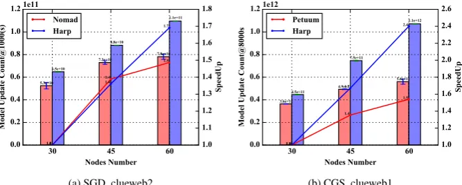
We further evaluate the scalability of Harp implementations by focusing on the com-parison between different implementations of CGS and SGD. We do not include CCD because regardless of whether we use Harp or CCD++, bothW andH model matrices are required to be synchronized rather than only rotatingHin SGD. There is more com-munication time than computation time per iteration, hence the iteration time does not decrease much when the scale goes up, resulting in low scalability.
Since the convergence speed is not linear as the execution time passes, we use throughput on the number of training data items processed to evaluate the scalability of CGS and SGD implementations. In SGD, the time complexity of processing a training data item isO(K)for all the elements inV; as such this metric is suitable for evaluating the performance of SGD implementations on different scales. Figure 4a shows that the throughput of Harp at 1000s achieves 1.7×speedup when scaling from 30 to 60 nodes. Meanwhile, NOMAD only achieves 1.5×speedup. The throughput of NOMAD on three scales are all lower than Harp. The situation on CGS is a little different. Since the time complexity of sampling each token isO(∑k1(Nwk6=0) +∑k1(Nk j6=0)), the time
com-plexity decreases during the convergence. As a result, the throughput on the number of tokens processed grows higher and higher as the execution time passes. When the dy-namic rotation control is applied, Harp can sample more tokens as the execution pro-gresses, which results in super linear speedup. Figure 4b shows the throughput of Harp and Petuum at 8000s. Harp has higher throughput than Petuum on the three scales.
5. Related Work
Much initial work on machine learning algorithms deploys one computation model and a single programming interface. Mahout13[10], Spark Machine Learning Library14, and Graph-based tools such as PowerGraph15[4] are three such examples. All these
imple-13
http://mahout.apache.org 14
https://spark.apache.org/docs/latest/mllib-guide.html
mentations are based on synchronized algorithms. Meanwhile, Parameter Server solu-tions [5][25][26] use asynchronous algorithms in which a programming interface allows each worker to “push” or “pull” model parameters for local computation. As mentioned in Section II, these solutions are not efficient for solving LDA and MF applications be-cause they use computation models with stale model parameters which do not converge as fast as solutions using model rotation [15].
Model rotation has been applied before in machine learning. In LDA, F. Yan et al. implement CGS on a GPU [27]. In MF, DSGD++ [22] and NOMAD [28] use model rotation in SGD for MF in a distributed environment while LIBMF [24] applies it to SGD on a single node through dynamic scheduling. Another work, Petuum STRADS [17][18][19], supplies a general parallelism solution called “model parallelism” through “schedule-update-aggregate” interfaces. This framework implements CGS for LDA us-ing model rotation but not CCD for MF16. Instead it uses “allgather” operation to collect model matricesW andHwithout using model rotation. Thus Petuum CCD cannot be ap-plied to big model applications due to the memory constraint. The interfaces of Petuum STRADS operate at the model parameter level but not in a collective way, resulting in communication inefficiency. Despite these shortcomings, Petuum LDA and NOMAD are still among the fastest implementations we know among open-source implementations of the two algorithms.
CCD++ uses a parallelization method on CCD different from either Petuum CCD or our model rotation implementation. CCD++ allows parallelization on updating different elements in a single feature vector ofW andH. In such a way, only one feature vector in
W and one feature vector inHare “allgathered”. Thus there is no memory constraint in CCD++ compared with Petuum CCD.
6. Conclusion
To solve big model problems in machine learning applications such as LDA and MF, this paper focuses on three algorithms, CGS, SGD and CCD, and gives a full solution using model rotation, which includes computation model innovation, programming interface design, and implementation improvements. For the algorithms without the “summation form”, we identify three important features in the model update mechanism and conclude that model rotation is more efficient compared to other computation models. We design the model rotation API with MapCollective programming interface which is more conve-nient than parameter-level APIs of other implementations. Finally, we use pipelining and dynamic rotation control to improve the efficiency of model rotation in CGS and SGD. With these steps, we achieve higher scalability and faster model convergence speed com-pared with related work. In the future, we can apply our model rotation solution to other large-scale learning applications with big models. Future research will also investigate providing templates for performance to guide developers to parallelize different machine learning applications based on data, algorithm, and hardware.
Acknowledgment
We gratefully acknowledge support from Intel Parallel Computing Center (IPCC) Grant, NSF 1443054 CIF21 DIBBs 1443054 Grant, and NSF OCI 1149432 CAREER Grant. We appreciate the system support offered by FutureSystems.
References
[1] Y. Wanget al., “Peacock: Learning Long-Tail Topic Features for Industrial Applications,”ACM TIST, 2015.
[2] J. Dean and S. Ghemawat, “MapReduce: Simplified Data Processing on Large Clusters,”CACM, 2008. [3] J. Ekanayakeet al., “Twister: A Runtime for Iterative MapReduce,” inHPDC, 2010.
[4] J. E. Gonzalezet al., “Powergraph: Distributed Graph-Parallel Computation on Natural Graphs,” in
OSDI, 2012.
[5] M. Liet al., “Scaling Distributed Machine Learning with the Parameter Server,” inOSDI, 2014. [6] B. Zhang, Y. Ruan, and J. Qiu, “Harp: Collective Communication on Hadoop,” inIC2E, 2015. [7] T. L. Griffiths and M. Steyvers, “Finding Scientific Topics,”PNAS, 2004.
[8] Y. Korenet al., “Matrix Factorization Techniques for Recommender Systems,”Computer, 2009. [9] H.-F. Yuet al., “Scalable Coordinate Descent Approaches to Parallel Matrix Factorization for
Recom-mender Systems,” inICDM, 2012.
[10] C.-T. Chuet al., “Map-Reduce for Machine Learning on Multicore,” inNIPS, 2007.
[11] L. Yao, D. Mimno, and A. McCallum, “Efficient Methods for Topic Model Inference on Streaming Document Collections,” inKDD, 2009.
[12] L. Bottou, “Large-Scale Machine Learning with Stochastic Gradient Descent,” inCOMPSTAT, 2010. [13] Q. Hoet al., “More Effective Distributed ML via a Stale Synchronous Parallel Parameter Server,” in
NIPS, 2013.
[14] R. Levine and G. Casella, “Optimizing Random Scan Gibbs Samplers,”JMVA, 2006.
[15] B. Zhang, B. Peng, and J. Qiu, “Model-Centric Computation Abstractions in Machine Learning Appli-cations,” inBeyondMR, 2016.
[16] D. Newmanet al., “Distributed Algorithms for Topic Models,”JMLR, 2009.
[17] S. Leeet al., “On Model Parallelization and Scheduling Strategies for Distributed Machine Learning,” inNIPS, 2014.
[18] E. P. Xinget al., “Petuum: A New Platform for Distributed Machine Learning on Big Data,”IEEE Transactions on Big Data, 2015.
[19] J. K. Kimet al., “STRADS: A Distributed Framework for Scheduled Model Parallel Machine Learning,” inEuroSys, 2016.
[20] B. Rechtet al., “HOGWILD!: A Lock-Free Approach to Parallelizing Stochastic Gradient Descent,” in
NIPS, 2011.
[21] R. Gemullaet al., “Large-Scale Matrix Factorization with Distributed Stochastic Gradient Descent,” in
SIGKDD, 2011.
[22] C. Teflioudi, F. Makari, and R. Gemulla, “Distributed Matrix Completion,” inICDM, 2012.
[23] B. Zhang, B. Peng, and J. Qiu, “High Performance LDA through Collective Model Communication Optimization,” inICCS, 2016.
[24] Y. Zhuanget al., “A Fast Parallel SGD for Matrix Factorization in Shared Memory Systems,” inRecSys, 2013.
[25] A. Smola and S. Narayanamurthy, “An Architecture for Parallel Topic Models,”VLDB, 2010. [26] A. Ahmedet al., “Scalable Inference in Latent Variable Models,” inWSDM, 2012.
[27] F. Yan, N. Xu, and Y. Qi, “Parallel Inference for Latent Dirichlet Allocation on Graphics Processing Units,” inNIPS, 2009.